Geographically weighted spatial interaction (GWSI)

(GWSI)

Maryam Kordi

A Thesis Submitted for the Degree of PhD

at the

University of St Andrews

2013

Full metadata for this item is available in

St Andrews Research Repository

at:

http://research-repository.st-andrews.ac.uk/

Please use this identifier to cite or link to this item:

http://hdl.handle.net/10023/4112

Geographically Weighted Spatial Interaction (GWSI)

Maryam Kordi

A Thesis submitted

for the degree of Doctor of Philosophy

at the

Centre for GeoInformatics (CGI)

School of Geography and Geosciences

University of St Andrews

I, Maryam Kordi, hereby certify that this thesis, which is approximately 42,001 words in length, has been written by me, that it is the record of work carried out by me and that it has not been submitted in any previous application for a higher degree.

I was admitted as a research student in October 2011 and as a candidate for the degree of PhD in October 2011; the higher study for which this is a record was carried out in the University of St Andrews between 2011 and 2013.

Date signature of candidate

Supervisor’s declaration:

I hereby certify that the candidate has fulfilled the conditions of the Resolution and Regulations appropriate for the degree of PhD in the University of St Andrews and that the candidate is qualified to submit this thesis in application for that degree.

giving permission for it to be made available for use in accordance with the regulations of the University Library for the time being in force, subject to any copyright vested in the work not being a↵ected thereby. I also understand that the title and the abstract will be published, and that a copy of the work may be made and supplied to any bona fide library or research worker, that my thesis will be electronically accessible for personal or research use unless exempt by award of an embargo as requested below, and that the library has the right to migrate my thesis into new electronic forms as required to ensure continued access to the thesis. I have obtained any third-party copyright permissions that may be required in order to allow such access and migration, or have requested the appropriate embargo below.

The following is an agreed request by candidate and supervisor regarding the elec-tronic publication of this thesis: Embargo on both all of printed copy and elecelec-tronic copy for the same fixed period of two years on the following ground: publication would preclude future publication.

One of the key concerns in spatial analysis and modelling is to study and analyse similar-ities or dissimilarsimilar-ities between places over geographical space. However, ”global“ spatial models may fail to identify spatial variations of relationships (spatial heterogeneity) by assuming spatial stationarity of relationships. In many real-life situations spatial varia-tion in relavaria-tionships possibly exists and the assumpvaria-tion of global stavaria-tionarity might be highly unrealistic leading to ignorance of a large amount of spatial information. In con-trast, local spatial models emphasise di↵erences or dissimilarity over space and focus on identifying spatial variations in relationships. These models allow the parameters of mod-els to vary locally and can provide more useful information on the processes generating the data in di↵erent parts of the study area.

In this study, a framework for localising spatial interaction models, based on geo-graphically weighted (GW) techniques, has been developed. This framework can help in detecting, visualising and analysing spatial heterogeneity in spatial interaction systems. In order to apply the GW concept to spatial interaction models, we investigate several approaches di↵ering mainly in the way calibration points (flows) are defined and spa-tial separation (distance) between flows is calculated. As a result, a series of localised geographically weighted spatial interaction (GWSI) models are developed.

Using custom-built algorithms and computer code, we apply the GWSI models to a journey-to-work dataset in Switzerland for validation and comparison with the related global models. The results of the model calibrations are visualised using a series of conventional and flow maps along with some matrix visualisations. The comparison of the results indicates that in most cases local GWSI models exhibit an improvement over the global models both in providing more useful local information and also in model performance and goodness-of-fit.

To my parents, Pedar va Madar e azizam

and to mon cher mari Christian.

I am forever grateful for your unconditional love and support.

First, I would like to express my sincere thanks to everyone who contributed in many ways to the success of this study, both at work and in my private life.

I gratefully thank my thesis supervisor, Professor A. Stewart Fotheringham, for his support and guidance throughout my PhD research. I am very much thankful to him for providing me this opportunity to pursue my doctorate under his supervision and also for providing necessary resources to accomplish my research work. I also gratefully thank him for providing me with the freedom to explore and try new ideas which made my PhD study an unforgettable experience. I can never thank Professor Fotheringham enough for his help and support with my transferring to St Andrews and during my residence in Cellardyke.

I would also like to extend my appreciation to my examining committee members: Prof. Graham Clarke from School of Geography, University of Leeds and Dr. Urˇska Demˇsar from Centre for GeoInformatics (CGI), University of St Andrews.

I also wish to thank everyone in the National Centre for Geocomputation (NCG) at the National University of Ireland Maynooth (NUIM) where I started my PhD study. My special thanks go to Martin Charlton, Dr. Alexei Pozdnoukhov and Dr. Carson Farmer who were always available for answering my academic questions and to Melina and Ann-Marie for their friendship and help during my study in NCG.

Finally I would like to express my gratitude to the faculty and sta↵ in the School of

Geography & Geosciences at University of St Andrews and also gratefully acknowl-edge my friends and colleagues in CGI. I truly appreciate Sila’s and Tommy’s o↵er for staying in their place whenever I traveled to St Andrews in the last few months of my PhD study.

1 Introduction 1

1.1 Motivation . . . 1

1.2 Aim and objectives of the thesis . . . 3

1.3 Short review of techniques and contributions of the thesis . . . 4

1.4 Outline of the thesis . . . 6

2 Data and case study 8 2.1 Introduction . . . 8

2.2 Subdivisions of Switzerland . . . 8

2.2.1 Agglomerations in Switzerland . . . 9

2.3 The Swiss journey-to-work (commuting) dataset in the literature . . . 9

2.4 A spatial interaction model for journey-to-work . . . 10

2.5 Case study: Lausanne . . . 12

3 Spatial flow modelling: an overview 22 3.1 Introduction . . . 22

3.2 General form and elementary components of spatial interaction modelling 23 3.3 Gravity model: an early spatial interaction model . . . 24

3.4 Entropy maximisation and the family of spatial interaction models . . . . 26

3.5 Utility maximisation . . . 30

3.6 Competing destination model . . . 31

3.7 Calibration of spatial interaction models . . . 32

3.8 Poisson spatial interaction model and maximum likelihood . . . 34

3.9 Journey-to-work Poisson gravity model in Lausanne . . . 37

3.10 Spatial flow modelling outside geography . . . 39

3.11 Zoning problems in spatial interaction . . . 41

3.12 Visualisation of spatial interaction . . . 42

4 Intra-zonal trip length in spatial interaction models 44 4.1 Introduction . . . 44

4.2 Background . . . 45

4.2.1 Circular-shape distance estimates . . . 46

4.3 Scattered intra-zonal distance estimates . . . 47

4.3.1 Randomly scattered distance estimates . . . 48

4.3.2 Density-based scattering approach . . . 51

4.4 Application & Results . . . 53

4.5 Summary . . . 55

5 Local spatial analysis 57 5.1 Introduction . . . 57

5.2 Overview of local methods for spatial data analysis . . . 59

5.3 Geographically Weighted Regression (GWR) . . . 61

5.3.1 Spatial weighting function . . . 62

5.3.2 Calibration of the spatial weighting function . . . 63

5.3.3 Geographically weighted Poisson regression (GWPR) . . . 65

5.4 Local calibration of spatial interaction models . . . 67

5.4.1 Origin-specific spatial interaction model . . . 68

5.4.2 Destination-specific spatial interaction model . . . 71

5.4.3 Local calibration of spatial interaction based on a GWR approach 74 6 Geographically weighted spatial interaction (GWSI) 80 6.1 Introduction . . . 80

6.2 Origin-focused GWSI approach . . . 80

6.2.1 Application of the origin-focused GWSI approach . . . 84

6.3 Destination-focused GWSI approach . . . 90

6.3.1 Application of the destination-focused GWSI approach . . . 92

6.4 Destination-specific origin-focused GWSI approach . . . 98

6.4.1 Application of the destination-specific origin-focused GWSI approach100 6.5 Origin-specific destination-focused GWSI approach . . . 104

6.5.1 Application of the origin-specific destination-focused GWSI approach108 6.6 Summary . . . 111

7 GWSI: Flow-focused approach 118 7.1 Introduction . . . 118

7.2 Flow-focused GWSI approach . . . 118

7.2.1 A four-dimensional kernel approach . . . 120

7.2.2 Spatial trajectories approach . . . 123

7.3 Application of the local flow-focused model to Lausanne journey-to-work data . . . 124

7.3.1 Bandwidth selection . . . 124

7.3.2 Adaptive spatial kernels . . . 125

8 Discussion and examples 139

8.1 Network distance and travel time approaches . . . 139

8.2 Mixed kernel approach . . . 141

8.2.1 Strength of connection as a similarity measure between destinations 142 8.2.2 Integrating destination similarity into the weighting function . . . 142

8.2.3 Example application of a mixed kernel . . . 144

8.2.4 Discussion of the mixed kernel approach . . . 145

8.3 GWSI: Scattered approach . . . 146

8.3.1 Origin-focused approach for Poisson spatial interaction using scattered-based method . . . 147

8.4 Adaptive bandwidth . . . 149

8.5 Application examples of the GWSI models . . . 151

8.5.1 Evaluate impact of new business centre . . . 151

8.5.2 Estimating commuting flows based on historic data . . . 155

8.5.3 Discussion of locational analysis examples . . . 156

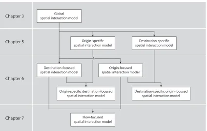
1.1 Overview of the spatial interaction models discussed in the thesis, with

their dependencies. . . 6

2.1 Agglomerations of Switzerland for year 2000 . . . 10

2.2 Overview map of the agglomeration of Lausanne . . . 13

2.3 Communes of the agglomeration of Lausanne . . . 14

2.4 Population of the agglomeration of Lausanne in 2000 . . . 15

2.5 Active population of the agglomeration of Lausanne in 2000 . . . 15

2.6 Number of jobs in the agglomeration of Lausanne in 2001 . . . 16

2.7 Number of jobs (2001) minus active population (2000) in the agglomera-tion of Lausanne. Proporagglomera-tional symbols depict the absolute value of the di↵erence. . . 16

2.8 Percentage of internal flows compared to the total of inflows for the com-munes of the agglomeration of Lausanne . . . 17

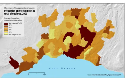
2.9 Percentage of internal flows compared to the total of outflows for the com-munes of the agglomeration of Lausanne . . . 18

2.10 Journey-to-work flows in the agglomeration of Lausanne, 2000 . . . 19

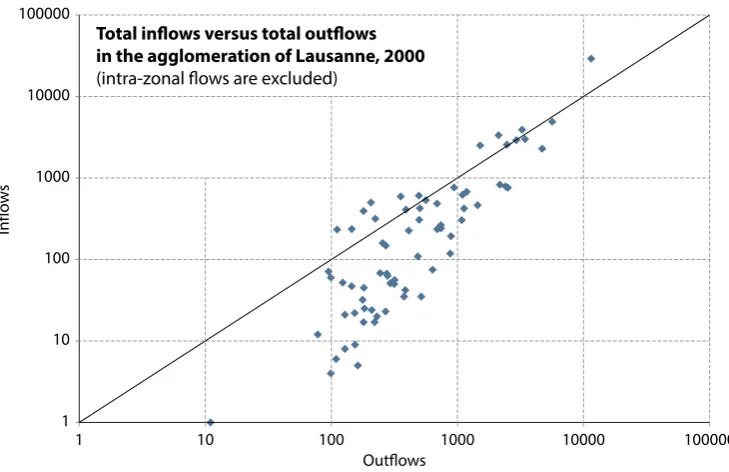
2.11 Inflows versus outflows in the agglomeration of Lausanne, 2000 . . . 19

2.12 Frequency histogram of the commuting distance in the agglomeration of Lausanne, 2000 . . . 20

2.13 Median income in the agglomeration of Lausanne, 2005 . . . 21

3.1 Simple spatial interaction system with some possible flow configurations. . 26

4.1 Example of average polygon distance. . . 49

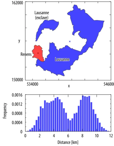
4.2 Average polygon distance between Lausanne and Renens. . . 51

4.3 Estimating the average trip length using a regular grid. . . 52

4.4 Predicted flows vs. observed flows for di↵erent distance measures. . . 56

5.1 A simplified illustration of the origin-specific spatial interaction. . . 69

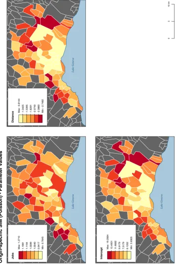
5.2 The parameter values for Poisson origin-specific model in agglomeration of Lausanne. . . 72

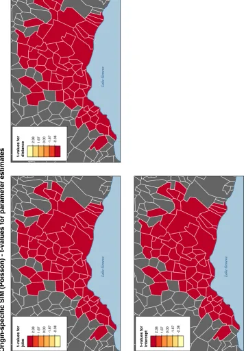
5.3 The t-values of the parameters for Poisson origin-specific model in agglom-eration of Lausanne. These maps display absolute t-values, where values greater than 2.33 are significant at a level of 99%, and values greater than 1.65 are significant at a level of 95%. For negative parameter values (for the distance decay parameter), the negative t-values of -2.33 and -1.65

correspond to the significance levels of 99% and 95% respectively. . . 73

5.4 A simplified illustration of the destination-specific spatial interaction. . . 74

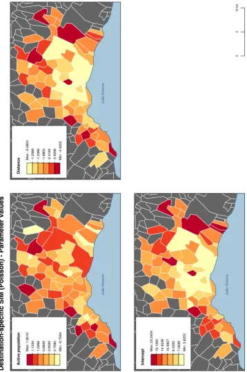
5.5 The parameters values for Poisson destination-specific model in

agglomer-ation of Lausanne. . . 75

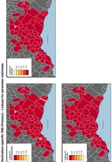
5.6 The t-values of parameters for Poisson destination-specific model in

ag-glomeration of Lausanne. These maps display absolute t-values, where values greater than 2.33 are significant at a level of 99%, and values greater than 1.65 are significant at a level of 95%. For negative parameter values (for the distance decay parameter), the negative t-values of -2.33 and -1.65

correspond to the significance levels of 99% and 95% respectively. . . 76

6.1 A schematic overview of the origin-focused GWSI approach. . . 82

6.2 Comparison between squared Cauchy and Gaussian kernel functions. . . . 85

6.3 Bandwidth value (fixed) against AICc, BIC and deviance for Poisson

origin-focused GWSI in Lausanne agglomeration, using a squared Cauchy

weighting function. . . 86

6.4 The parameter estimates of the Poisson origin-focused GWSI model over

all communes of the Lausanne agglomeration. . . 89

6.5 The t-values of parameters of the Poisson origin-focused GWSI model over

all communes of the Lausanne agglomeration. These maps display absolute t-values, where values greater than 2.33 are significant at a level of 99%, and values greater than 1.65 are significant at a level of 95%. For negative parameter values (for the distance decay parameter), the negative t-values of -2.33 and -1.65 correspond to the significance levels of 99% and 95%

respectively. . . 91

6.6 A schematic overview of destination-focused GWSI approach. . . 92

6.7 Bandwidth value (fixed) against deviance, AICc and BIC score for Poisson

destination-focused model in Lausanne agglomeration, using a squared

Cauchy weighting function. . . 93

6.8 The parameter estimates for Poisson destination-focused GWSI model in

6.9 The t-values of parameters for Poisson destination-focused GWSI model in agglomeration of Lausanne. These maps display absolute t-values, where values greater than 2.33 are significant at a level of 99%, and values greater than 1.65 are significant at a level of 95%. For negative parameter values (for the distance decay parameter), the negative t-values of -2.33 and -1.65

correspond to the significance levels of 99% and 95% respectively. . . 96

6.10 A simplified illustration of the destination-specific origin-focused GWSI

approach. . . 99

6.11 Optimal bandwidth for destination-specific origin-focused GWSI models. . 101 6.12 Distance-decay parameter of the destination-specific origin-focused GWSI

for Lausanne agglomeration. Each row (destination) represents one destination-specific origin-focused model, calibrated separately for each origin (col-umn), resulting in 4900 di↵erent parameter estimates. . . 102 6.13 Active population parameter of the destination-specific origin-focused GWSI

for Lausanne agglomeration. Each row (destination) represents one destination-specific origin-focused model, calibrated separately for each origin (col-umn), resulting in 4900 di↵erent parameter estimates. . . 103 6.14 The t-values of distance-decay parameter of the destination-specific

origin-focused GWSI for Lausanne agglomeration. This map displays absolute t-values, where values smaller than -2.383 are significant at a level of 99%, and values smaller than -1.668 are significant at a level of 95%, and values smaller than -1.294 are significant at a level of 90%. Each row (destina-tion) represents one destination-specific origin-focused model, calibrated separately for each origin (column), resulting in 4900 di↵erent t-values. . . 105 6.15 The t-values for active population parameter of the destination-specific

origin-focused GWSI for Lausanne agglomeration. This map displays ab-solute t-values, where values greater than 2.383 are significant at a level of 99%, and values greater than 1.668 are significant at a level of 95%, and values greater than 1.294 are significant at a level of 90%. Each row (desti-nation) represents one destination-specific origin-focused model, calibrated separately for each origin (column), resulting in 4900 di↵erent t-values. . . 106

6.16 The PseudoR2 of the destination-specific origin-focused GWSI models for

Lausanne agglomeration. Each row (destination) represents one destination-specific origin-focused model, calibrated separately for each origin

(col-umn), resulting in 4900 di↵erent PseudoR2 values. . . 107

6.19 Distance-decay parameter of the origin-specific destination-focused GWSI for Lausanne agglomeration. Each row (origin) represents one origin-specific destination-focused model, calibrated separately for each desti-nation (column), resulting in 4900 di↵erent parameter estimates. . . 112 6.20 The t-values for the distance-decay parameter of the origin-specific

destination-focused GWSI for Lausanne agglomeration. This map displays absolute t-values, where values smaller than -2.383 are significant at a level of 99%, and values smaller than -1.668 are significant at a level of 95%, and values smaller than -1.294 are significant at a level of 90%. Each row (origin) rep-resents one origin-specific destination-focused model, calibrated separately for each destination (column), resulting in 4900 di↵erent t-values. . . 113 6.21 Number of jobs parameter of the origin-specific destination-focused GWSI

for Lausanne agglomeration. Each row (origin) represents one origin-specific destination-focused model, calibrated separately for each desti-nation (column), resulting in 4900 di↵erent parameter estimates. . . 114 6.22 The t-values for number of jobs parameter of the origin-specific

destination-focused GWSI for Lausanne agglomeration. This map displays absolute t-values, where values greater than 2.383 are significant at a level of 99%, and values greater than 1.668 are significant at a level of 95%, and values greater than 1.294 are significant at a level of 90%. Each row (origin) rep-resents one origin-specific destination-focused model, calibrated separately for each destination (column), resulting in 4900 di↵erent t-values. . . 115

6.23 The PseudoR2 of the origin-specific destination-focused GWSI models for

Lausanne agglomeration. Each row (origin) represents one origin-specific destination-focused model, calibrated separately for each destination

(col-umn), resulting in 4900 di↵erent PseudoR2 values. . . 116

7.1 The set of points at equal distance r from a given point A wherer is a:

(a.) Euclidean distance, (b.) city-block distance and (c.) Chebyshev distance. . . 121

7.2 The flow (ij) and (i0j0) represented as a four-dimensional vector in

Eu-clidean space. . . 122

7.3 Distance(p1· · ·pn, q1· · ·qn) =

n P

t=1k

pt qtk . . . 124

7.4 Bandwidth value (fixed) against AICc score for the Poisson flow-focused

model in Lausanne agglomeration. Deviance and BIC are also shown. . . 125

7.5 Adaptive bandwidth value (number of flows considered) against AICc score

7.6 Parameter↵, active population, using the bandwidth of 1318 metres. Each cell shows the parameter value of one flow-focused model, corresponding to the destination (row) and the origin (column) of each flow. The resulting matrix visualisation shows the parameter values of all 4900 calibrated models.129

7.7 Parameter , number of jobs, using the bandwidth of 1318 metres. Each

cell shows the parameter value of one flow-focused model, corresponding to the destination (row) and the origin (column) of each flow. The resulting matrix visualisation shows the parameter values of all 4900 calibrated models.130

7.8 Parameter , distance-decay, using the bandwidth of 1318 metres. Each

cell shows the parameter value of one flow-focused model, corresponding to the destination (row) and the origin (column) of each flow. The resulting matrix visualisation shows the parameter values of all 4900 calibrated models.131

7.9 Distance decay parameters for inflows in 5 communes in the agglomeration

of Lausanne. The value of the parameter estimates are represented by di↵erent colours and the width of the lines shows original flow data values (flow size). . . 132 7.10 Active population parameters (alpha) for inflows in 5 communes in the

agglomeration of Lausanne. The value of the parameter estimates are represented by di↵erent colours and the width of the lines shows original flow data values (flow size). . . 134 7.11 Number of jobs parameters (gamma) for inflows in 5 communes in the

agglomeration of Lausanne. The value of the parameter estimates are represented by di↵erent colours and the width of the lines shows original flow data values (flow size). . . 135 7.12 Distance decay parameters for outflows from 5 communes in the

agglomer-ation of Lausanne. The value of the parameter estimates are represented by di↵erent colours and the width of the lines shows original flow data values (flow size). . . 136 7.13 Active population parameters (alpha) for outflows from 5 communes in

the agglomeration of Lausanne. The value of the parameter estimates are represented by di↵erent colours and the width of the lines shows original flow data values (flow size). . . 137 7.14 Number of jobs parameters (gamma) for outflows from 5 communes in

the agglomeration of Lausanne. The value of the parameter estimates are represented by di↵erent colours and the width of the lines shows original flow data values (flow size). . . 138

8.1 Weighting of flows in a destination-focused approach is done using the

8.2 Bandwidth optimisation plot using AICc for both spatial and strength of connection bandwidths, with a weight of 0.8 for the spatial kernel and 0.2 for the strength of connection kernel. . . 144

8.3 Plot showing the AICc for di↵erent weights of the spatial kernel, for spatial

bandwidth of 200 metres and strength of connection bandwidth of 0.2. . . 145

8.4 Flows from regioni stacked at the centroid of the region. . . 146

8.5 Bandwidth value (fixed) against AICc score for the origin-focused Poisson

model using stacked and the scattered-based method. . . 147

8.6 The median parameter estimates for origin-focused Poisson model using

scattered-based method. . . 148

8.7 The median t-values of parameters for origin-focused Poisson model using

scattered-based method. These maps display absolute t-values, where val-ues greater than 2.33 are significant at a level of 99%, and valval-ues greater than 1.65 are significant at a level of 95%. For negative parameter values (for the distance-decay parameter), the negative t-values of -2.33 and -1.65 correspond to the significance levels of 99% and 95% respectively. . . 150

8.8 Bandwidth value (adaptive; number of flows) against AICc for

origin-focused Poisson model. . . 151

8.9 Bandwidth value (adaptive; number of flows) against AICc for

origin-focused Poisson model using scattered approach. . . 152 8.10 Location of the fictional new business centre in the agglomeration of

Lau-sanne . . . 153

8.11 Bandwidth selection plot for the destination-focused model using a squared Cauchy kernel. . . 153 8.12 Estimated flows based on the destination-focused model calibrated at the

location of the business centre. . . 154 8.13 Estimated flows based on the origin-specific destination-focused model

cal-ibrated at the location of the business centre, corrected using a total-flow constraint. . . 155 8.14 Bandwidth selection plot for the flow-focused model with squared Cauchy

kernel. . . 156 8.15 Estimated flows in 2000 based on the flow-focused model (top left),

di↵er-ence of estimated and observed flows in 2000 (top right), estimated flows in 2010 (bottom left) and estimated increase in commuting flows from 2000

to 2010 (bottom right). . . 157

3.1 Origin-destination matrix . . . 24

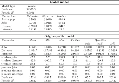
3.2 Global Poisson gravity model for journey-to-work in agglomeration of

Lau-sanne . . . 38

4.1 Estimating the distance between two polygons . . . 49

4.2 Estimating the distance between two polygons (Lausanne and Renens). . 52

4.3 Comparison of di↵erent methods for calculating average trip length

(dis-tance). The results show the output from calibrating a spatial interaction

model with the di↵erent distance estimates. . . 54

5.1 The Poisson global and origin-specific models for journey-to-work in the

agglomeration of Lausanne. . . 70

5.2 The Poisson destination-specific model for journey-to-work in the

agglom-eration of Lausanne. . . 74

6.1 Poisson origin-specific and origin-focused GWSI models . . . 87

6.2 Poisson destination-specific and destination-focused GWSI models . . . . 94

7.1 Poisson flow-focused GWSI model, with fixed bandwidth of 1318 metres,

and four-dimensional squared Cauchy kernel . . . 127

8.1 Global Poisson spatial interaction model with di↵erent distance measures 140

8.2 Poisson flow-focused model with di↵erent distance measures . . . 140

8.3 Origin-focused GWSI (Poisson with scattered origins) . . . 149

8.4 Poisson origin-specific destination-focused GWSI model . . . 154

Introduction

1.1

Motivation

Spatial interaction is broadly defined as the movement, flow, or communication of peo-ple, goods or information over space resulting from a decision-making process (Haynes and Fotheringham, 1984; Fotheringham and O’Kelly, 1989; Fotheringham et al., 2000; Fotheringham, 2001; Fischer, 2000). Examples include a wide variety of behaviours such as migration, shopping patterns, commuting, commodity or communication flows, tele-phone calls, airline passenger traffic, attendance at events such as theatre, conferences and sport events (Haynes and Fotheringham, 1984), all of which form important com-ponents of social and urban complex systems. Researchers in a variety of fields have modelled spatial movements through mathematical equations known as spatial interac-tion models (Fotheringham et al., 2000). These models are particularly useful for better understanding and analysing the patterns of and the underlying structure of the spatial flows in the interaction systems. One of the early spatial interaction models was the grav-ity model and its related family of models (Wilson, 1967, 1970; Haynes and Fotheringham, 1984; Fotheringham and O’Kelly, 1989; Sen and Smith, 1995; Fotheringham et al., 2000; Roy and Thill, 2004). Later, the underlying formulations of spatial interaction models have been modified further and more sophisticated models have been developed such as competing destinations models (see Fotheringham, 1983, 1984b, 1986).

Spatial interaction is fundamental in regional science (Fischer and Getis, 1999; Clarke and Clarke, 2001) and is also an important aspect of modern society and economy. As a consequence, spatial interaction modelling is one of the most applied geographical anal-ysis and modelling techniques (Fotheringham et al., 2000) (see for instance applications and references in Fotheringham and O’Kelly, 1989; Haynes and Fotheringham, 1984). Traditionally, spatial interaction models have been calibrated globally in which one set of parameter estimates is provided for a study region (Fotheringham and Brunsdon, 1999). The resulting global parameter estimates represent an average type of interaction behaviour and are assumed to be equally valid across the entire study area. The global validity of the results is due to the assumption of spatial stationarity in relationships

being investigated (Lloyd, 2011). However, in many real-life situations relationships may vary across space and then important variations in interaction behaviour could be com-pletely hidden (Linneman, 1966; Greenwood and Sweetland, 1972; Fotheringham et al., 2000, 2002) because the global results may fail to represent the true specification of the reality (Fotheringham and Brunsdon, 1999; Fotheringham et al., 2002; Unwin, 1996a,b; Fotheringham, 1997; Boots and Okabe, 2007).

The global model misspecification came to light through local parameter estimates being obtained for each separate origin or destination region (Fotheringham et al., 2000, 2002) (see sections 5.4.1 and 5.4.2 for further information). The origin- and destination-specific models provide a set of parameter estimates for each origin or destination in the system (see for instance Haynes and Fotheringham, 1984; Fotheringham and O’Kelly, 1989). Although the origin- and destination-specific models provide more disaggregated information compared to global interaction models, these models are localised at the level of discrete origins/destinations. An important drawback of these models is the fact that they ignore a substantial amount of data that can be potentially useful for calibration. For example, an origin-specific model ignores flows from surrounding origins that might have similar flows to the destinations, leading to a lower number of considered data points and potentially to a less reliable parameter estimation. Another possible problem with origin- and destination-specific models is the fact that these models might ignore significant geographical variations of parameters in the interaction system. For example, an origin-specific model provides a single set of parameters for a given origin, ignoring potential di↵erences across destinations. Therefore, identifying spatial variations in relationships, (sometimes referred to as spatial heterogeneity, spatial non-stationarity or spatial drift (Charlton et al., 1997)), is still an ongoing problem in spatial interaction modelling requiring further study. This leads to the following research questions:

• How can spatial heterogeneity be detected and taken into account in spatial

inter-action processes?

• How can spatial interaction models be localised to consider spatial heterogeneity?

in section 5.3. Within the GWR framework, relationships under study are allowed to vary spatially and a set of local parameter estimates is produced for each regression lo-cation and all observations are spatially weighted with respect to the regression point. The GWR technique has been used in a wide range of applications for spatial data (see section 5.4.3) and found to be efficient in detecting spatial heterogeneity in relationships that may be missed in a global regression analysis (Foody, 2004). The local parameter estimates derived from a GWR analysis can be mapped to show how a relationship varies over space and then to investigate the spatial pattern of the local estimates for better understanding of possible causes of this pattern (Fotheringham et al., 2002).

Considering that GWR could successfully contribute to modelling “spatially hetero-geneous processes” (Brunsdon et al., 1996; Fotheringham et al., 1996, 1997b, 2002) and has efficiently worked in a range of studies for spatial data, questions we are therefore addressing are:

• How it is possible to use the experience from GWR in order to apply the geographical

weighting concept to spatial interaction models?

• Within a geographically weighting framework for spatial interaction, how do we

define distances between spatial flows?”

• How do we visualise the local parameter estimates for spatial interaction models?

On a practical side, given the availability of GWR software, the following question is of interest:

• Will existing GWR software work for spatial interaction flows or is a specific

adap-tation to spatial interaction required?

Given the importance of intra-zonal flows in many spatial interaction processes, and the local nature of assessing spatial heterogeneity, we also include the following important question into this research:

• How can intra-zonal trip distance be estimated in spatial interaction systems in

which intra-zonal flows are taken into account in the analysis?

1.2

Aim and objectives of the thesis

The aim of this research is to develop a framework for localising spatial interaction models using the geographically weighted concept (known from GWR) in which spatial heterogeneity can be detected, visualised and analysed in spatial interaction systems.

The following research objectives represent the required steps for achieving this aim:

• Designate and specify a real-world spatial interaction problem for the case study

• Explore and investigate di↵erent existing spatial interaction models.

• Investigate possible ways to incorporate intra-zonal flows in the spatial interaction

models along with exploring and analysing existing approaches.

• Study and analyse the spatial interaction patterns of the case study using both

global and existing local techniques.

• Explore possible approaches for applying the geographically weighted concept to

spatial interaction models.

• Create an algorithm and, if necessary, write computer code for calibrating

geo-graphically weighted spatial interaction (GWSI) models.

• Perform verification and validation of the GWSI models by applying them to the

case study for detecting and analysing spatial heterogeneity.

• Develop and apply appropriate techniques for the visualisation of the conventional

and local interaction model results.

• Analyse and compare the spatial patterns of the parameter estimates resulting from

global and various local models.

• Demonstrate some application examples of the GWSI models especially for the case

of forecasting spatial interaction patterns.

1.3

Short review of techniques and contributions of the

thesis

The idea of applying the GWR approach to spatial flows was pointed out by Berglund

and Karlstr¨om (1999) where the potential applicability of this approach was suggested

Therefore, the question of “how to apply the geographically weighted concept on spatial interaction models” still remains unsolved.

In order to fulfil the main aim of this study which is to develop a framework for localising spatial interaction models using the geographically weighted concept, we have investigated several approaches di↵ering mainly in the way calibration points (flows) are defined and spatial separations (distance) between flows are estimated. As result, a family of geographically weighted spatial interaction (GWSI) models is developed throughout this thesis allowing for the detection of spatial variations in interaction behaviour. The family of GWSI models is composed of the following local models:

• Origin-focused spatial interaction model

• Destination-focused spatial interaction model

• Destination-specific origin-focused spatial interaction model

• Origin-specific destination-focused spatial interaction model

• Flow-focused spatial interaction model

In all these models, following the principle of the geographically weighing concept, around each calibration point a spatial kernel is considered and observations are weighted ac-cording to their proximity to the calibration point. However, the main di↵erence between the models is the way the calibration point and the distances between flows are defined. In the first four models, the resulting local parameter estimates are associated with the spatial flows, although the calibration points in the geographically weighting approach are actual locations within the study region; i.e. origin locations in the case of origin-focused models and destination-specific origin-origin-focused models, and destination locations in the case of destination-focused models and origin-specific destination-focused models. The distance between flows is defined by the distance between the calibration point and origins or destinations of the observed flows in the origin-focused and destination-focused models respectfully.

The flow-focused model is di↵erent from others because the calibration points in the geographically weighting approach are spatial flows. Therefore, in a flow-focused model a spatial kernel is considered around each calibration flow and the observed flows within this kernel are weighted. Two feasible ways for estimating distances between flows are suggested in this thesis; one based on a four-dimensional spatial kernel and one based on a spatial trajectory distance measure.

Chapter 3

Chapter 5

Chapter 7 Chapter 6

Global spatial interaction model

Origin-specific spatial interaction model

Flow-focused spatial interaction model

Destination-specific spatial interaction model

Destination-focused

spatial interaction model spatial interaction modelOrigin-focused

Origin-specific destination-focused

spatial interaction model Destination-specific origin-focusedspatial interaction model

Figure 1.1: Overview of the spatial interaction models discussed in the thesis, with their dependencies.

improvement over the global models both in providing more useful local information and also in terms of model performance and goodness-of-fit.

Figure 1.1 gives a visual overview of the di↵erent spatial interaction models discussed in this thesis and relates them to each other. An additional contribution of this work is the discussion on how intra-zonal flows can be considered in spatial interaction models by introducing a method for intra-zonal distance measures. Internal flows are important in local spatial interaction models, because these local flows will be given more weight in a geographically weighting procedure since they are always closer to the calibration location compared to other observed flows. Also, the Lausanne journey-to-work dataset contains an important proportion of internal flows (about 45%), which is an additional reason to include these flows in the models.

1.4

Outline of the thesis

This thesis is structured in 9 chapters, as follows:

• In chapter 2 we introduce the dataset of journey-to-work in the Lausanne

agglomer-ation in Switzerland which is used throughout the work in order to test and validate the interaction models.

theoretical framework along with a discussion on calibration techniques for the interaction models. Also a global Poisson gravity model is calibrated using the journey-to-work dataset in Lausanne described in chapter 2.

• In chapter 4 we discuss the intra-zonal flows problem and introduce a methodology

for estimating the average zonal trip length allowing for integration of intra-zonal flows in spatial interaction models.

• Chapter 5 gives a brief overview of the existing local methods for spatial data

analysis with attention given to the models which are used in this thesis such as Geographically Weighted Regression (GWR) and origin- and destination-specific spatial interaction models.

• Chapter 6 combines the geographically weighted concept with spatial interaction

models and introduces four members of a family of local GWSI models: origin-focused, destination-origin-focused, destination-specific origin-origin-focused, and origin-specific destination-focused models and discusses their application to the Lausanne journey-to-work dataset.

• Chapter 7 introduces the last version of the GWSI, flow-focused model and discusses

distance measures between flows along with bandwidth calibration and spatial ker-nel issue. This model is also applied to the Lausanne journey-to-work dataset and the results are briefly analysed.

• Chapter 8 discusses some further issues around local spatial interaction and shows

some example applications where GWSI models are used for prediction.

• Chapter 9 concludes the thesis by giving a short overview of the models and the

Data and case study

2.1

Introduction

This thesis focuses on the methodologies of localising spatial interaction models. In order to illustrate and examine local interaction methods we need to use an appropriate spatial dataset. Spatial interaction, by definition, takes place between a pair of locations in space (i.e. origin and destination points) and data should contain information on the volume of flows between these points as well as attributes and locational information about the origins and destinations (see Thompson, 1974; Bailey and Gatrell, 1995; Banerjee et al., 2000; Rae, 2009). Here in this study, the data are used only for model validation and exposition so the ideas herein are not limited to any particular type of spatial interaction data but instead have broad application.

The Swiss Federal Statistical Office provides fine scale data on journey-to-work (com-muting) between di↵erent communes in the country. Communes, also known as munici-palities, are the smallest administrative district in Switzerland. In order to provide more detailed information about the dataset, we first describe some general definitions and information about the subdivisions of Switzerland.

2.2

Subdivisions of Switzerland

There are several administrative divisions in Switzerland that divide the country into smaller units. The highest administrative subdivision in the country are known as can-tons. There are 26 cantons in Switzerland which are the member states of the Swiss Confederation. Each canton is divided in a number of districts and each district is di-vided in communes which is the smallest administrative unit. Switzerland had 2896 communes in 2000. Communes have a local government and are responsible for basic public services. Communes vary in the size from 22 residents for Corippo (Ticino) to 363,273 residents for the city of Zurich (for year 2000, data from Population Census 2000).

Besides the administrative levels of cantons, districts and communes, Switzerland is

divided in a series of other spatial subdivisions based on several statistical variables. One of these subdivisions is the concept of agglomeration, corresponding roughly to what is a Metropolitan Area in the US (Berry et al., 1969; Dahmann and Fitzsimmons, 1995). Other countries have very similar concepts, for instance the Urban Areas in the UK.

2.2.1 Agglomerations in Switzerland

The agglomerations try to define the spatial extent of urban areas. According to Schuler et al. (2005, published by Federal Swiss Statistical Office), the definition of agglomerations is based on di↵erent characteristics. More specifically, in Switzerland, a commune belongs to an agglomeration if at least 3 of the 5 following criteria are met:

• Continuity of built zone with the central city

• High human density (sum of residential population and number of jobs)

• Population growth higher than average

• Low agricultural activity

• Strong commuting relationships with the central zone of the agglomeration

Figure 2.1 shows the Swiss agglomerations according to the definition of the year 2000. They contain a central city (in red) and surrounding functionally and economically de-pendent areas (in orange). In some particular cases, an agglomeration can also consist of a single isolated city (in yellow). The main purpose of the definition of agglomera-tions is to be able to compare urban areas with very di↵erent administrative limits. All agglomerations together define the urban area of Switzerland, as opposed to rural zones. With progressing urbanisation, the definition of agglomeration has changed over time and is periodically updated by the Swiss Federal Statistical Office (usually every 10 years). In some cases, an agglomeration can also contain neighbouring areas abroad where the functional and economic relationships are strong. A total of 979 of 2896 communes were considered as being ’urban‘ in 2000, with a total of 73% of the population (Schuler et al., 2005).

2.3

The Swiss journey-to-work (commuting) dataset in the

literature

0 20 km

Source: Swiss Federal Statistical Office, 2000 Agglomerations of Switzerland (2000)

Rural communes Central city of agglomeration Agglomeration commune Isolated city

Unproductive land Agglomeration border Canton border

Lausanne

Bern

Zurich

Lucerne

Chur

Lugano

St. Gallen Basel

Sion Fribourg

Geneva

Figure 2.1: Agglomerations of Switzerland for year 2000

dataset also contains information about the means of transportation used for the journey to work. Kanevski et al. (2009) have used these data to illustrate the ability of Gen-eral Regression Neural Networks (GRNN) to predict the spatial pattern of the usage of di↵erent means of transportation in commuting. The data has also been used for visuali-sation purposes in Killer and Axhausen (2010) or Kaiser (2011). Kaiser et al. (2011) have used the commuting dataset to demonstrate the calibration of a local spatial interaction model using a variant of geographically weighted regression. Dessemontet et al. (2010) have made an extensive study of the commuting network of Switzerland by using the same dataset and Dessemontet (2011) has used these journey-to-work data along with other data to study the evolution of employment and accessibility in Switzerland over 60 years.

2.4

A spatial interaction model for journey-to-work

housing markets are connected through commuting flows and so the size of flows between regions and their e↵ect on the housing and labour markets can be analysed with spatial interaction models (see Batten and Boyce, 1986; Fotheringham and O’Kelly, 1989).

A comprehensive introduction to spatial interaction modelling is given in section 3. However, briefly there are three essential elements in spatial interaction models. The first is travel cost which often is measured as distance between interaction (origin and destination) regions; the second and third elements are attributes (or sizes) of interac-tion regions which measure propulsiveness of origins and attractiveness of destinainterac-tions respectively. Based on the type of interaction problem and the purpose of the model, di↵erent origins and destinations attributes can be considered in the model. For instance in a shopping expenditure model, the origin attribute might be defined as the average household income or unemployment rate whereas in a migration model, living cost or average house price can be considered as destination attributes (see Fotheringham and O’Kelly, 1989).

In this thesis, according to the available elements in our dataset, we consider four components in our journey-to-work model. The first component is that of commuting flows which will act as the independent variable in the calibration of the spatial interaction model. The other three components are:

- Number of economically active population (working people) in each commune, con-sidered as an origin propulsiveness attribute

- Number of jobs in each destination region, considered as a destination attractiveness attribute

- Euclidean distance between centroids of origin and destination communes, consid-ered as a surrogate for travel cost

Although the selection of variables in the interaction case study in this work is mainly guided by available census elements, there are a number of studies in the literature using the same variables for commuting analysis, supporting these choices (see for instance Uboe, 2004; Lloyd and Shuttleworth, 2005; Shuttleworth and Lloyd, 2005; O’Kelly and Niedzielski, 2007, 2008; Lloyd et al., 2007).

In this thesis we use the Swiss commuting dataset for the year 2000 which was the latest available version of the data at the time of analysis. This dataset is issued from the population census, which contains also other data including population. The number of jobs is available through the firms census which has been conducted during 2001. The qualifying date for the population census 2000 is the 5 December, while the firms census contains data for the 1 January 2001, less than one month later. The following sentences give a summary of general information about the data used in this thesis for spatial interaction modelling:

• The journey-to-work data were acquired during the population census 2000. Frick

data acquisition and descriptive statistics. The Swiss Federal Statistical Office

o↵ers this commuting data at the fine communal level, freely available at http:

//www.pendlerstatistik.admin.ch

• Information about active population has been acquired during the population

cen-sus 2000, along with other information such as residential population. Most of the

data from the population census is freely available at http://www.stattab.bfs.

admin.ch at the level of the communes, including the active population we are

using for our case study.

• The number of jobs has been acquired by the Statistical Office during the firms

census in 2001, where information about all companies in Switzerland was collected. Information about the economic sectors is also available, including the split of the number of jobs between secondary and tertiary sectors. Again, most of the data

from this census is also freely available athttp://www.stattab.bfs.admin.ch at

the level of the communes.

2.5

Case study: Lausanne

The agglomeration of Lausanne, located in Western Switzerland was selected as the study area for the calibration of various spatial interaction models. This agglomeration

is composed of 70 communes, covering a total area of roughly 317 km2 with a population

of slightly more than 310,000. The agglomeration is well separated from neighbouring agglomerations which limits undesired inter-agglomeration interactions. Also the agglom-eration of Lausanne does not extend behind the country borders as it is the case in some areas in Switzerland; e.g. in the agglomeration of Geneva where over 9% of the workforce lives in France, or in Basel where over 13% of the workforce lives in France or Germany. In Lausanne only 1% of commuters are cross-border. Consisting of 70 communes with populations ranging from 61 inhabitants (commune of Malapalud) up to 124,914 for the city of Lausanne, (overall population about 310,000 in 2000), makes the agglomeration of Lausanne the 5th biggest agglomeration in Switzerland. Figure 2.2 shows an overview of the agglomeration of Lausanne with the road and train network. Lausanne is bordered in the south by Lake Geneva. The main transportation routes are along the lake and also in a northerly direction.

Lake G

enev

a

LA

USANNE

LA

USANNE

Communes of the agglomer

ation of L

ausanne Map da ta fr om O penS treetMap , C C-B Y-SA 2.0, do wnloaded fr om geofabrik .de Railw ay Mot or wa y Primar y r oad Sec ondar y r oad Ter tiar y r oad Residen tial r oad For est

O

ver

view map of the agglomer

ation of Lausanne

0 5 km Source: Swisstopo, VECTOR200, 2013 Lausanne Morges Epalinges Cugy Pully Paudex Belmont VilletteGrandvaux Cully Savigny Montpreveyres Les Cullayes Mézières Servion Carrouge Villars-Tiercelin Froideville Bottens Poliez-le-Grand Malapalud Assens St-Barthélémy Bioley-Orjulaz Boussens Etagnières Cheseaux Romanel- sur-Lausanne Jouxtens-Mézéry Chavannes Ecublens St-Sulpice Crissier Bussigny Prilly Renens Bretigny Morrens Echallens Lutry Le Mont-sur-Lausanne Lausanne (exclave) Villars-St-Croix Mex Sullens Daillens Penthalaz Penthaz Vuffl

ens-la-Ville Aclens Bremblens Echandens Denges Lonay Echichens Chigny Vuffl ens-le-Château Denens Bussy-Chardonney Villars- sous-Yens Lussy Etoy Buchillon Aubonne Lully Tolochenaz St-Prex Prévérenges Romanel-sur-Morges St-Saphorin-sur-Morges Cossonay

70 communes of the agglomeration of Lausanne

L a k e G e n e v a

Figure 2.3: Communes of the agglomeration of Lausanne

population together with the people seeking actively employment, students are not con-sidered in the active population unless they are working part time. The spatial structure of the active population is similar to the residential population; the city of Lausanne has an active population of nearly 60,000 which is roughly 38% of the overall active popula-tion in the agglomerapopula-tion. The ratio of active populapopula-tion to residential populapopula-tion is of 48% in the city of Lausanne, and 50% in the whole agglomeration.

Figure 2.6 shows the number of jobs in the agglomeration in 2001. A job is considered as an occupied working place in a company so vacant jobs are not counted in this statistic. There is also no di↵erence between part time and full time jobs; both are counted as a job. Nearly half of the jobs (roughly 86,000 of 175,500, or 48.9%) are located in the city of Lausanne, which shows its important role as a centre of this agglomeration. The remaining jobs are mainly located in the west and north-west of the city, not far from the junction of the motorways going east, west and north. Figure 2.7 compares the number of jobs with the active population. Blue circles depict a surplus of jobs, while red circles represent communes with a greater number of population than jobs. This map shows a clear gap between the economic and the residential communes in the agglomeration. The communes east of Lausanne are typical residential communes with a wealthier population.

Figures 2.8 and 2.9 both show the percentage of internal flows for each commune.

In figure 2.8, the number of internal flows is compared to the total incoming flows to

0 5 km Source: Swiss Federal Statistics Office, Population census, 2000

Residential population, 2000 70 communes of the agglomeration of Lausanne

L a k e G e n e v a

20’000 Number of people

Minimum: Malapalud (61) Maximum: Lausanne (124’914)

10’000 5’000 1’000

Figure 2.4: Population of the agglomeration of Lausanne in 2000

0 5 km Source: Swiss Federal Statistics Office, Population census, 2000

Active population, 2000 70 communes of the agglomeration of Lausanne

L a k e G e n e v a 20’000

Number of people

Minimum: Malapalud (30) Maximum: Lausanne (59’599)

10’000 5’000 1’000

0 5 km Source: Swiss Federal Statistics Office, Firms census, 2001

Number of jobs, 2000 70 communes of the agglomeration of Lausanne

L a k e G e n e v a

20’000 Number of people

Minimum: Malapalud (25) Maximum: Lausanne (85’912)

10’000 5’000 1’000

Figure 2.6: Number of jobs in the agglomeration of Lausanne in 2001

0 5 km Source: Swiss Federal Statistics Office, Firms census, 2001 Difference of number of jobs and

active population, 2000 70 communes of the agglomeration of Lausanne

L a k e G e n e v a

Number of jobs minus active population Minimum: Pully (-2940) Maximum: Lausanne (26313)

1000 100 2500 5000

Number of jobs higher than active population Active population bigger than number of jobs

absolute values

0 5 km Source: Swiss Federal Statistics Office, Population census, 2000 Proportion of internal flows to

total of inflows, 2000 70 communes of the agglomeration of Lausanne

L a k e G e n e v a

Percentage of internal flows compared to the total of inflows

Max: Malapalud (93.3%)

Min: Mex (8.8%) 28% 42% 60% 75%

Figure 2.8: Percentage of internal flows compared to the total of inflows for the communes of the agglomeration of Lausanne

flows is computed compared to the total outgoing flows. Figure 2.8 gives information on

the percentage of the commuters, working in a commune living in this same commune. As an example, from the 64,717 people commuting to Lausanne, 35,585 or 55% live in Lausanne itself. The spatial pattern shows clearly that the smaller communes at the border of the agglomeration have a high percentage of internal flows compared to the total of incoming flows, suggesting few people commute to these communes. On the other hand, the communes west of Lausanne have more jobs than active population (see also figure 2.7) and typically have a high percentage of people commuting from other communes. The information in figure 2.9 represents the percentage of workforce staying inside their commune of residence for their work. As an example, from the 47,071 commuters of the city of Lausanne, 35,585 or 75.6% do not leave the city for employment. This percentage of internal flows compared to the total of outflows is higher than average in the communes having more jobs than active population. But there are a series of communes in the western border of the agglomeration towards Geneva showing even higher proportions of internal flows to total of outflows. These communes seem to o↵er a high proportion of jobs to the local population while having, with the exception of Aubonne, a surplus of active population compared to the number of jobs, which is rather unusual in the agglomeration of Lausanne.

0 5 km Source: Swiss Federal Statistics Office, Population census, 2000

Proportion of internal flows to total of outflows, 2000 70 communes of the agglomeration of Lausanne

L a k e G e n e v a Percentage of internal flows

compared to the total of outflows Max: Lausanne (75.6%)

Min: Bretigny (12.9%) 19% 24% 32% 50%

Figure 2.9: Percentage of internal flows compared to the total of outflows for the com-munes of the agglomeration of Lausanne

represented by proportional circles while the inter-zonal flows are depicted by lines with proportional width. The map shows clearly an inner part of the agglomeration which is very well connected in terms of journey-to-work flows. This inner part runs roughly from Morges in the West to Lutry in the East and contains the communes North-West of Lausanne having more jobs than active population (see figure 2.7). The communes in the inner part of the agglomeration are well connected between themselves, while the flows in the surrounding communes focus mainly towards the inner part of the agglomeration. This pattern shows a concentric organisation of the agglomeration where the central part has the biggest parts of the jobs, and the surrounding communes are mostly residential.

Figure 2.11 shows the relationship between the total incoming versus the total outgo-ing flows. The diagonal line represents equality of incomoutgo-ing and outcomoutgo-ing flows. Both axes of the chart have logarithmic scales. Only a few communes have higher inflows than outflows. This chart shows that a few central communes have more jobs than active pop-ulation, and many small, less central communes are typical residential communes with much more outflows than inflows.

0 5 km Source: Swiss Federal Statistics Office, Population census, 2000 Journey-to-work flows, 2000

70 communes of the agglomeration of Lausanne

L a k e G e n e v a

Intra-zonal flows

5000 1000 10000

Inter-zonal flows

Only flows with more than 20 commuters are depicted

1000 300 100

Figure 2.10: Journey-to-work flows in the agglomeration of Lausanne, 2000

Total inflows versus total outflows in the agglomeration of Lausanne, 2000

(intra-zonal flows are excluded)

Outflows

In

fl

ow

s

100000

10000

1000

100

10

1

1 10 100 1000 10000 100000

Commuting distance

Frequency

0 5 km 10 km 15 km 20 km 25 km

0

10000

20000

30000

40000

50000

60000

Figure 2.12: Frequency histogram of the commuting distance in the agglomeration of Lausanne, 2000

most of the internal flows are in reality not of distance 0, this results in a under-estimation of the commuting distance. Neverthless, figure 2.12 shows an exponential decrease in the frequency of the flows with increasing distance.

Another interesting map describing the median income of the resident population in the agglomeration of Lausanne in 2005 is shown in figure 2.13. The data are provided by the tax administration of the canton of Vaud. The number of communes in the agglomeration has been reduced to 65 in 2005, as some communes have merged with neighbouring communes. According to the map, residents of city of Lausanne have the lowest income. This is perhaps due to more students and lower-income workers living here. This is also true for the communes west of the city of Lausanne such as Renens, Prilly or Ecublens. In contrast, the commune of Jouxtens-M´ezery located just in the north of Lausanne is the commune with the highest median income. This is possibly because of the low tax rate in this commune in comparison with other parts of the agglomeration which make this commune an attractive place to live for wealthier people. The communes of Saint-Sulpice and Buchillon in the middle south and west are famous for being wealthy locations lying along Lake Geneva.

0 5 km Source: Administration cantonale vaudoise des impôts, SCRIS, 2012 Median income of the population, 2005

65 communes of the agglomeration of Lausanne (spatial division of 2012)

L a k e G e n e v a Median income [CHF]

Max: Jouxtens-Mézery (118,431 CHF)

Min: Lausanne (55,588 CHF) 68,000 CHF 78,000 CHF 85,000 CHF 98,000 CHF

Figure 2.13: Median income in the agglomeration of Lausanne, 2005

these variables are used to produce the maps presented in this chapter.

Spatial flow modelling: an

overview

3.1

Introduction

According to Fotheringham and O’Kelly (1989); Fischer (2000) and Fotheringham (2001),

spatial interaction can be broadly defined asthe movement or communication of objects

such as people, goods and information over geographic space that results from a

decision-making process (also Batten and Boyce, 1986). By this definition, spatial interaction

covers a wide variety of behaviours and movements such as migration, shopping trips, commuting, commodity or communication flows, trips for educational purposes, airline passenger traffic, the choice of health care services, the spatial pattern of telephone calls, emails and the World Wide Web connections and even attendance at events like conferences, cultural and sport events (Haynes and Fotheringham, 1984). All of these behaviours form important components of social and urban complex systems. In each

case, an individual or group of individuals trade o↵the benefit of the interaction with the

cost of overcoming the separation between them and their possible destinations; hence, these decision-making processes are particularly related to spatial choice. The decision where to relocate in case of migration, where to shop in case of shopping and the decision where to live or where to work in case of journey-to-work are examples of spatial choice in spatial interaction.

Usually spatial interaction systems are complex and multi-dimensional; according

to Van-Lierop (1986), this could be due to the fact that”in reality, multiple dimensions

are involved in the geographical dispersion of human activities and the spatial relation-ship between them“. This sort of complex system is difficult to model and analyse. It has been shown that even simple spatial interaction processes can show complex, chaotic behaviour (see e.g. Dendrinos and Sonis, 1990; Chen, 2009). However, to facilitate under-standing and analysis of the patterns and underlying structures of spatial flows in inter-action systems, during the years, researchers in various fields have tried to model spatial

flows through mathematical equations, known broadly as ”spatial interaction models“. Spatial interaction models can be used for explanatory purposes when each determi-nant of flows is examined through an associated parameter estimate (Fotheringham and O’Kelly, 1989). These models also can provide the opportunity to predict flows patterns when changes in the interaction system occur; e.g. in a shopping behaviour model, to forecast how patterns of spatial flows will change when a shop in the study area either opens or closes.

In this chapter an overview of spatial interaction models is provided with the following structure: the general form and basic elements of the interaction models are described in section 3.2; the gravity model is introduced in section 3.3 as an early spatial interaction model; entropy and utility maximisation frameworks of spatial interaction models are presented in sections 3.4 and 3.5 respectively; section 3.7 covers the calibration tech-niques for interaction models and includes the Poisson form of spatial interaction model; and in a final section of 3.9, a Poisson gravity model is applied to journey-to-work flows in Lausanne, as an empirical example of a global interaction model.

3.2

General form and elementary components of spatial

interaction modelling

The most general form of a spatial interaction model can be formulated (see e.g. Wilson,

1967; Alonso, 1978; Sen and S¨o¨ot, 1981) as:

Tij =f(Vi Wj Cij) (3.1)

where the interaction between any pair of origins iand destinationsj is specified asTij,

Vi represents a vector of origin factors measuring the propulsiveness of origin i, Wj is

a vector of destination attractiveness factors, and Cij represents a vector of separation

factors, measuring the separation between zonesiandj usually in term of distance, cost

or travel time betweeniand j (Fischer, 2000; Haynes and Fotheringham, 1984).

In spatial interaction analysis, a so-called ”origin-destination matrix“ is often used

to display the interactions between di↵erent origins and destinations. The size of this matrix is defined by the number of origins and destinations in the interaction system.

Table 3.1 represents an origin-destination matrix for an interaction system withmorigins

and n destinations. The elements, Tij, of this (m⇥n) matrix indicate the number of

flows between originiand destinationj. Each row of the matrix is allocated to an origin

iand the columns are aligned with each destinationj. The total number of interactions

emanating from each originiand the total interactions terminating in each destinationj

are summed in correspondingOi rows and Dj columns respectively; the sum of all flows

in the matrix which represents the total number of interactions in the system is shown

by T in table 3.1 (for a reference see e.g. Van-Lierop, 1986). Besides Tij, the variables

Vi, Wj and Cij of a spatial interaction model (see equation 3.1) can also be represented

Table 3.1: Origin-destination matrix

`````<sub>`````</sub>

``

Origin

Destination

1 2 3 · · · n Total

1 T11 T12 · · · T1n O1

2 T21 T22 · · · T2n O2

3 · · · ·

· · · ·

· · · ·

· · · ·

· · · ·

· · · ·

m Tm1 Tm2 · · · Tmn Om

Total D1 D2 · · · Dn T

system withmorigins andndestinations, an (m_⇥p) matrixV and an (q_⇥n) matrixW

can be used for representing origin and destination attributes respectively, and a (m⇥n)

matrixC where its elementscij represent separation between origini and destinationj

(generally in terms of distance) can be considered as components in spatial interaction models (Fotheringham and O’Kelly, 1989):

V = 0 B B B B @ v1

1 v21 · · · v

p

1

v1

2 v22 · · · v

p

2

..

. ... ... ...

v1

m v2m · · · vpm

1 C C C C

A W =

0 B B B B @ w1

1 w21 · · · w1n

w2

1 w22 · · · w2n

..

. ... ... ...

wq1 w

q

2 · · · wqn

1 C C C C

A C=

0 B B B B @

c11 c12 · · · c1n

c21 c22 · · · c2n

..

. ... ... ...

cm1 cm2 · · · cmn

1 C C C C A

3.3

Gravity model: an early spatial interaction model

One of the most widely used modelling frameworks for spatial interaction is the Gravity model (Haynes and Fotheringham, 1984) which has a long history in the social sci-ences (Sen and Smith, 1995), and for which many review texts exist (e.g. Roy and Thill, 2004; Sen and Smith, 1995; Batten and Boyce, 1986; Roy, 2004). The early attempts of understanding regularities in patterns of spatial flows, which can be seen as the starting point of gravity models, date back at least to the works of Carey (1858) and Ravenstein (1885) who observed a greater number of migrants to move between larger and closer

cities,ceteris paribus (O’Kelly, 2009; Fotheringham et al., 2000).

The essence of the gravity model framework is based on Newton’s law of universal gravitation: the attraction between every entity is proportional to their masses and inversely proportional to their distance. During the mid-1850s, Newton’s theory began to be used for modelling certain types of human activity between entities physically separated in geographical space (Roy and Thill, 2004). In determining spatial interaction based on Newton’s theory, initially the gravitational force was replaced with the number

of interactions between originiand destinationj asTij; the masses were specified by the

measured sizes of the interaction regions, for example by their populations: Pifor origins