Phase field Simulation of Transient Liquid Phase Bonding Process of Ni Using Ni P Binary Filler Metal

Phase-field Simulation of Transient Liquid Phase Bonding Process

of Ni Using Ni–P Binary Filler Metal

Yukinobu Natsume

_{, Kenichi Ohsasa and Toshio Narita}

The transient liquid phase (TLP) bonding process of Ni using a Ni–11 mass%P binary filler metal was simulated by using both a phase-field model (PFM) and a moving boundary model (MBM). The dissolution of the base metal and isothermal solidification behavior during the TLP bonding process were simulated, and the results calculated by using the PFM were compared with those obtained by using the MBM. The results obtained during the isothermal solidification process in the two models were the same. The change in the concentration at the solid-liquid interface during the dissolution of the base metal was examined, and deviation from the local equilibrium concentration occurred in samples with a high heating rate in the phase-field simulation. On the other hand, the local equilibrium was always maintained in the MBM, but the calculation time of the simulation using the MBM was several hundred-times faster than that using the PFM.

(Received November 21, 2002; Accepted February 24, 2003)

Keywords: transient liquid phase bonding, phase-field, simulation, nickel, phosphorus, dissolution, isothermal solidification

1. Introduction

Transient liquid phase (TLP) bonding is a technique that was originally developed for bonding of Ni-base heat-resistant alloys, and a good bonding region having the same structure as the base metal with no heat-affected zone (HAZ) can be obtained by using this technique.1–3)The TLP bonding process, which is controlled by the diffusion of solute elements in liquid and solid, can be classified into three stages:4) (1) dissolution of a base metal, (2) isothermal solidification and (3) homogenization. In these stages, an isothermal holding stage requires the longest time in the entire bonding process and determines the overall bonding time. If isothermal solidification is not completed during the isothermal holding stage, liquid remains in the bonding region, and brittle eutectic or peritectic phases may form during the cooling stage and spoil the mechanical properties of the joint.1,3,5,6)The dissolution of the base metal is also an important factor because the isothermal solidification time is influenced by the amount of the dissolved region. In order to predict the optimum conditions for the real bonding opera-tion, it is important to clarify the effects of the process parameters on the dissolution of the base metal and subsequent isothermal solidification. However, many experi-mental works would be required to obtain the optimum conditions, and it is desirable to develop the mathematical model to simulate the TLP bonding process.

Several mathematical models, both analytical and numer-ical, have been presented to predict the TLP bonding process.7–10) The authors have also developed numerical models to simulate the TLP bonding process for binary and ternary systems and have examined the factors controlling the isothermal solidification process.7,8)Most of the proposed models, including the authors’ models, are one-dimensional moving boundary model assuming a local equilibrium at the solid-liquid interface. Although the assumption of a local equilibrium holds true for usual solidification processes such as casting, the solute distribution at the solid-liquid interface

will deviate from the equilibrium state during both rapid solidification and rapid dissolution processes. However, it is very difficult to introduce a non-equilibrium condition into a moving boundary model.

Recently, the phase-field method has been used as a powerful tool for solidification analysis.11–15) This method automatically satisfies the local equilibrium at the solid-liquid interface when the interface velocity is relatively low. The phase-field method is also known to produce solute trapping phenomena during rapid growth conditions. It may therefore be expected that the phase-field method can be used to predict the dissolution process of the base metal and subsequent isothermal solidification process under both the equilibrium and non-equilibrium states.

The aims of this study were: 1) to establish a basic one-dimensional phase-field model of the TLP bonding process and 2) to compare the dissolution and isothermal solidifica-tion behavior simulated using the phase-field model (PFM) and that simulated using the moving boundary model (MBM). The advantages and disadvantages of the two models were discussed in this paper.

2. Simulation Methods of the TLP Bonding Process

2.1 Phase-field model

Two governing equations, phase-field equation and diffu-sion equation, are used in a PFM. The governing equations of the PFM used for an alloy and the free energy density of a solid-liquid mixture,fðc; Þ, are expressed as follows.

@ @t ¼M "

2@ 2

@x2 f

; ð1Þ

@c

@t ¼

@

@x DðÞ

fcc

@fc

@x

; ð2Þ

fðc; Þ ¼hðÞfSðcSÞ þ ð1hðÞÞfLðcLÞ þWgðÞ; ð3Þ

whereis the phase field (¼0in liquid and¼1in solid)

hðÞ ¼3_ð151062_{Þ and gðÞ ¼}2_ð1Þ2_{; f}S _and fL_{are the free energy density of the solid and liquid phases,} *_{Graduate Student, Hokkaido University.}

Special Issue on Solidification Science and Processing for Advanced Materials

M1¼

Vm m

þ

DðÞpffiffiffiffiffiffiffi2Wðc e S;c

e

LÞ ; ð6Þ

ðce_S;c_LeÞ ¼f_ccSðce_SÞf_ccLðce_LÞðce_Lce_SÞ2

Z1

0

hðÞ½1hðÞ

½1hðÞfS

ccðceSÞ þhðÞfccLðceLÞ d

ð1Þ: ð7Þ

Here, is the interfacial energy, is the thickness of interface region, R is the gas constant, T is the absolute temperature, Vm is the molar volume, k is the partition

coefficient andis the kinetics coefficient.Mis a phase-field parameter related to the growth or dissolution kinetics of the solid-liquid interface. The derivation of phase-field para-meters is described in detail in a paper by Kimet al.15)

2.2 Moving boundary model

The MBM presented by Shinmuraet al.,7)in which a local equilibrium at the solid-liquid interface was assumed and the position of the solid-liquid interface is continuously deter-mined by calculating the diffusion in both liquid and solid, was used for simulation of the TLP bonding process. The basic equations used in the MBM are as follows:

ðCLCSÞ dXL=S

dt ¼ DL

@C

@X

XL=S þDS

@C

@X

XL=S

; ð8Þ

@C

@t ¼D

@2_C

@X2; ð9Þ

CL¼ TTm

m ; ð10Þ

CS¼kCL; ð11Þ

C¼CLfLþCð1fLÞ; ð12Þ

whereCLandCSare the equilibrium concentrations of liquid

and solid at the interface, respectively,XL=Sis the position of

the solid-liquid interface, DL and DS are the diffusion

coefficients of solute in liquid and solid, respectively,Tmis

the melting point of pure metal (here Ni), mis the slope of liquidus line,Cis the solute content of the grid in which the solid-liquid interface exists, and fLis the liquid fraction of

the grid.

2.3 Calculation procedure

A Ni–11 mass%P binary alloy was selected as the filler metal, and the TLP bonding process of Ni was calculated by using both the PFM and MBM. The physical properties of the Ni–P binary alloy used in the simulation are shown in Table 1. Because the thermodynamic data of a regular solution model for a Ni–P system could not be obtained from the literature, a dilute solution model was used as a free energy function for the Ni–P alloy, which is needed in the PFM calculation. Diffusion coefficients of the solute in liquid

and solid were calculated at each time step by eq. (13) to take account of the temperature dependence.

Di¼D0;iexp Qi

RT

; ð13Þ

whereD0is the frequency factor,Qis the activation energy, andidenotes liquid or solid. Since the diffusion coefficient of P in Ni was not found in the literature, the diffusion coefficient of P in austenite steel was used instead in the calculation. The diffusion coefficient of P in liquid Ni was also not found in the literature, and the value of P in molten iron therefore used instead. The partition coefficient of P determined from a published Ni–P binary alloy phase diagram16) is very small (k¼1:55102_{). Nakagawa et} al.9) reported that the results of calculation of the TLP bonding process in a Ni–P system using a small partition coefficient of P did not agree with the experimental results.9) Therefore, the partition coefficient of P for austenite (k¼0:13) was used in the present calculation, as it was in the work of Nakagawaet al.9)

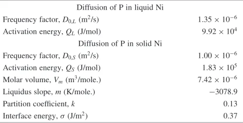
The following assumptions were considered to simulate the TLP bonding of Ni using a Ni–11 mass%P filler metal. First, because the solute diffuses in a direction perpendicular to the solid-liquid interface during the TLP bonding process, it was assumed that a one-dimensional calculation domain would be sufficient. Second, because the shape of the joint sample was symmetrical with respect to the center of the sample (Fig.1), it was assumed that only half of the sample would be sufficient for simulation. Third, it was assumed that densities of the solid and liquid were equal and constant. Table 1 Physical properties of the Ni–P binary alloy used in the

simulation.

Diffusion of P in liquid Ni

Frequency factor,D0;L(m2/s) 1:35106

Activation energy,QL(J/mol) 9:92104

Diffusion of P in solid Ni

Frequency factor,D0;S(m2/s) 1:00106

Activation energy,QS(J/mol) 1:83105

Molar volume,Vm(m3/mole.) 7:42106

Liquidus slope,m(K/mole.) 3078:9

Partition coefficient,k 0.13

Finally, it was assumed that dissolution and solidification proceed with planar solid-liquid interface morphology.

In order to solve eqs. (1), (2), (8) and (9) numerically by using the finite difference method, the samples for both the PFM and MBM were divided into one-dimensional grids along with the length of the samples. The sizes of grids in the PFM and MBM were 0.2mmand 1.0mm, respectively. The mathematical expressions for the boundary conditions at the center of the sample and the sample edge were as follows:

@C

@x ¼0; ð14Þ

@

@x ¼0: ð15Þ

Equation (15) was used only in the PFM, and eq. (11) was used in the MBM as the boundary condition at the solid-liquid interface.

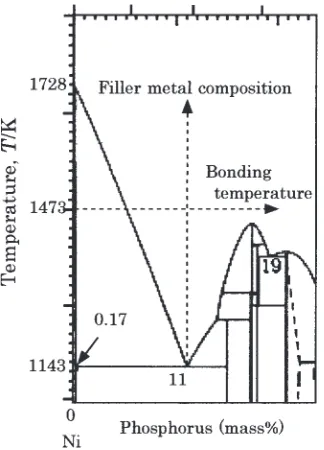
The bonding stages of the simulation were as follows: a sample was heated from the eutectic temperature of 1143 K (stage 1), held at 1473 K for a certain time (stage 2), and then cooled to the eutectic temperature (stage 3) (see Figs.2and 3). The bonding conditions are shown in Table2. The initial conditions at the solid-liquid interface in the PFM are ¼ 0:5and the eutectic concentration for the initial interface grid

and that in the MBM are the concentration of solid and liquid satisfied the local equilibrium at eutectic temperature.

3. Results and Discussion

3.1 Results of the simulation

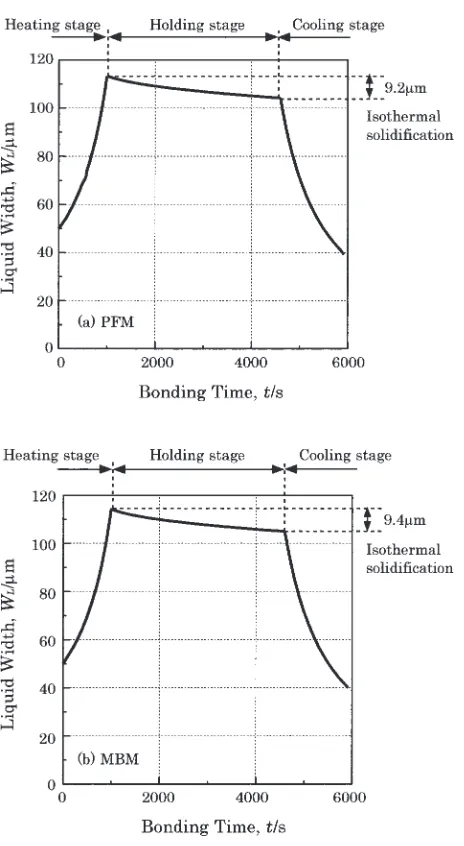
Figure4shows the changes in liquid width during the TLP bonding process for the two models. Figures 4(a) and (b) show the results of simulation using the PFM and MBM, respectively. The bonding conditions were TB¼1473K, tH¼3600s,RH¼0:33K/s,RC¼0:25K/s, and thickness of

the filler metal of 50mm. The maximum liquid widths of the dissolved base metal during the heating process were 113.4mm in the PFM and 114.0mm in the MBM. The following simple formula has been proposed for estimating the maximum liquid width,Wmax, under the condition of no diffusion in the solid:17)

Wmax¼ ðC0L=C B

LÞW0; ð16Þ

whereC0

Lis the initial concentration of the filler metal,CLBis

the concentration of liquid for the maximum liquid width, andW0is the initial thickness of the filler metal. The value of Wmaxestimated from eq. (16) was 114.7mmand was in good agreement with the values calculated from the two models, indicating that the effect of diffusion in the solid during the stage of dissolution of the base metal is negligible.

In the isothermal holding stage, the liquid width gradually decreased due to diffusion in the solid, and the total reductions in liquid width were 9.2mm in the PFM and 9.4mm in the MBM. Isothermal solidification was not completed under the bonding conditions used, and liquid of approximately 105mmin width for both models remained at the end of the isothermal holding stage. After the isothermal holding stage, the liquid width decreased due to solidification during the cooling stage, and the widths finally became 39.2mmin the PFM and 40.0mmin the MBM. The residual liquid was then transformed into a eutectic structure. Fig. 2 Ni–P equilibrium phase diagram.

Fig. 3 A schematic illustration of the thermal program for the TLP bonding process.

Table 2 Conditions used for the simulation of TLP bonding of Ni using a Ni–11 mass%P filler metal.

Bonding temperature,TB(K) 1473

Heating rate,RH(K/s) 0.33–33

Cooling rate,RC(K/s) 0.25

Holding time,tH(s) 3600

Thickness of filler metal (mm) 20–50 Fig. 1 A schematic illustration of the calculation domain used in the

3.2 Comparison of the PFM and the MBM

The calculated liquid width in the PFM was in good agreement with that in the MBM. The applicability of the PFM was confirmed because it has been reported that the results of calculation of the TLP bonding process using an MBM agreed well with the experimental results.7,8) How-ever, calculation using the PFM required CPU time of approximately 70 hours (Athlon 800 MHz PC) in the present work. When the MBM was used, the same results could be obtained in less than 10 minutes. The reasons of this difference in computation times are 1) the change in the phase field must be calculated in the PFM in addition to calculation of the diffusion field and 2) finer grids must be used in the PFM for numerical calculation of the solid-liquid interface region.

From the viewpoint of prediction of the isothermal solidification time, the MBM may be more useful than the PFM. The problem of the long computation time when using the PFM may be overcome by using an improved algorithm in making the code of the PFM and the development of a

high-performance computer in the near future. Fig. 5 Changes in liquid width during dissolution of the base metal at three heating rates, (a) 0.33 K/s (b) 3.3 K/s and (c) 33 K/s.

tion immediately after the end of the heating stage. The liquid width increased from the initial value of 20mmand reached the maximum value of about 45mmat the end of the heating stage. On the other hand, in the sample with the highest heating rate (33 K/s), the liquid width still kept on increasing after reaching the start of the isothermal holding stage (Fig. 5(c)). The maximum liquid width in this sample was 45.7mm, which is slightly larger than those of the other two samples with lower heating rates.

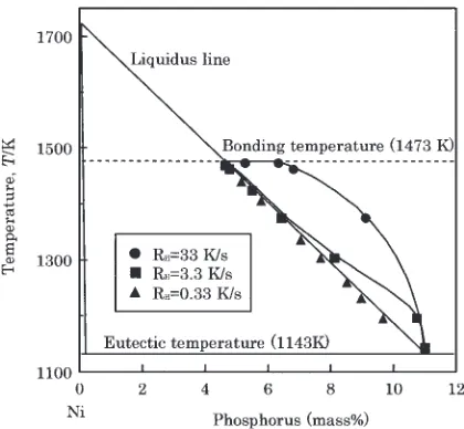
Figure6shows the changes in the concentrations in liquid at the solid-liquid interfaces of the samples with three heating rates during the heating stage. In the sample with the lowest heating rate (0.33 K/s), the liquid concentration changed along the equilibrium liquidus line from the eutectic to the bonding temperature. On the other hand, in the sample with highest heating rate (33 K/s), the liquid concentration deviated from the equilibrium concentration to a higher concentration region, and the liquid concentration reached an equilibrium concentration within a few seconds after the temperature had reached the bonding temperature. In the sample with a medium heating rate (3.3 K/s), the behavior was between that in the case of 0.33 K/s and that in the case of 33 K/s. These results indicate that in the case of a relatively high heating rate, the local equilibrium at the solid-liquid interface dose not hold true and that the concentrations in liquid and solid at the solid-liquid interface deviate from the equilibrium concentrations.

As shown above, the PFM enables prediction of the dissolution process at a high heating rate in which the local equilibrium dose not hold true. Thus, that the PFM should be used to analyze the process in which the effect of a non-equilibrium state is not negligible. On the other hand, for items in which the effect of a non-equilibrium state is not important, such as the prediction of isothermal solidification time, the MBM, which has high cost performance for CPU time as described in section 3.2, should be used.

4. Conclusions

Numerical simulations of the TLP bonding process of Ni using a Ni–11 mass%P binary filler metal were carried out by using a phase-field model and moving boundary model. The dissolution of the base metal and isothermal solidification behavior during the TLP bonding process were simulated. Based on the results of simulation, the comparison between the PFM and the MBM was carried out. The following results were obtained in this study:

(1) In the simulation of the dissolution process of the base metal with a high heating rate using PFM, deviation of the concentrations of P in liquid and solid at the solid-liquid interface from the equilibrium values occurred. (2) As a result of the non-equilibrium state, the maximum

dissolved liquid width in the sample with a high heating rate became slightly larger than that in the sample with a low heating rate in which the local equilibrium holds true.

(3) The MBM cannot be used for treating a non-equili-brium state because a local equilinon-equili-brium is assumed and incorporated in the model. However, the MBM has high cost performance for CPU time, and the computation time of simulation using the MBM is several hundred-times faster than that using the PFM.

REFERENCES

1) D. S. Duvall, W. A. Osczarski and F. Paulonis: Weld. J.53(1974) 203– 214.

2) J. T. Nieman and R. A. Garret: Weld. J. Research Suppl.53(1974) 175–184.

3) R. R. Wells: Weld. J. Research Suppl.55(1976) 20–27.

4) I. Tuah-Poku, M. Dollar and T. B. Massalski: Metall. Trans.19A

(1988) 675–686.

5) W. F. Gale and E. R. Wallach: Metall. Trans.22A(1991) 2451–2457. 6) R. Venkatraman, J. R. Wilcox and S. R. Cain: Metall. Trans.28A

(1997) 699–706.

7) T. Shinmura, K. Ohsasa and T. Narita: Mater. Trans.42(2001) 292– 297.

8) K. Ohsasa, T. Shinmura and T. Narita: J. Phase Equilibra20(1999) 199–206.

9) N. Nakagawa, C. H. Lee and T. H. North: Metall. Trans.22A(1991) 543–555.

10) C. E. Campbell and W. J. Boettinger: Metall. Trans.31A(2000) 2835– 2847.

11) R. Kobayashi: J. Cryst. Soc. Japan18(1991) 209–216. 12) R. Kobayashi: Physica D63(1993) 410–423.

13) J. A. Warren and W. J. Boettinger: Acta Metal. Mater.43(1995) 689– 703.

14) J. S. Lee and T. Suzuki: ISIJ Int.39(1999) 246–252.

15) S. G. Kim, W. T. Kim and T. Suzuki: Phys. Rev. E60(1999) 7186– 7197.

16) K. J. Lee and P. Nash: BINARY ALLOY PHASE DIAGRAMS 3

(1990) 2833–2835.

17) K. Saida, Y. Zhou and T. H. North: J. Japan Inst. Metals58(1994) 810– 818.