Abstract—Construction cost estimation is essential for turnkey construction. The good estimate should be a fair price for both customer and construction company. This research aims to compare the cost estimates of electrical and communication system for industrial factory construction. Three forecasting methods compared in this research are Multiple Regression Analysis (MRA), Multiple Regression Analysis incorporating Genetic Algorithm (MRA-GA), and Neural Network (NN). The data sets are collected from 31 industrial factory projects constructed in Thailand between year 2005 and 2011 which are divided into 25 training data sets and 6 testing data sets. The selected input variables are area, cost percentage from copper, cost percentage from main equipment, cost percentage from labor, and air condition system. The results show that MRA-GA model provides slightly lower root mean squared error (RMSE) than MRA and NN models.
Index Terms— Cost Estimation, Multiple Regression Analysis, Genetic Algorithm, Neural Network
I. INTRODUCTION
The accurate construction cost estimation is crucial for construction projects [1]-[3]. It plays an important role in the success of the project since it is a fundamental of the engineering projects [4]. It is well known that approximately 70% of the cost is determined in the early design phases [3] since the core structural systems and construction materials are set in this stage [2].
Reference [4] divided the construction design phase into three stages including preliminary planning stage, planning stage, and detail design stage. The in-situ investigations and identified demands will be used to draft the preliminary plan. The overall cost estimate is then generated and checked for the accuracy. After that, in the planning stage, the initial design will be developed and confirmed with the client’s demands. The cost estimate will be categorized in detail. Finally, the detail design will be done in the last stage. The cost estimation in this paper will be in the second stage (planning stage) which the construction cost estimate will be more accurate than the preliminary planning stage.
Manuscript received on June 6, 2012.
N. Kantanantha is a lecturer at Industrial Engineering Department, Faculty of Engineering, Kasetsart University, Bangkok, 10900, Thailand (corresponding author; e-mail: [email protected]).
P. Leelakriangsak is a graduate student in Engineering Management Program, Industrial Engineering Department, Faculty of Engineering, Kasetsart University, Bangkok, 10900, Thailand (e-mail: [email protected]).
The objective of this paper is to compare the accuracy of the cost estimates of electrical and communication system for industrial factory construction. The estimation methods performed in this study are Multiple Regression Analysis (MRA), Multiple Regression Analysis incorporating Genetic Algorithm (MRA-GA), and Neural Network (NN).
The organization of this paper is as follows. Section II reviews the relevant literature. The data and accuracy measurement are presented in Section III. In Section IV, the models are developed and the results of three methods are compared. Finally, the conclusions are drawn in Section V.
II. LITERATURE REVIEW A. Multiple regression analysis
The multiple regression analysis (MRA) has been used in cost estimation since 1970s [5], [6]. The regression model is generally formulated in the form of:
0 1 1 2 2 n n
y
x
x
x
(1) where y is the dependent variable, e.g. the estimated cost, and x1,x2,…,xn are independent variables related to cost estimation. The examples of the independent variables are floor area, number of storeys, types of building, etc.
is an error. β0 is the constant whereas β1,β2,…,βn are the coefficients. These coefficients will be estimated by the regression model.The applications of MRA in cost estimation can be found in various constructions, e.g. office [7], highway [8], rail [9], power generation [10], and wastewater treatment facilities [11].
Reference [6] developed two regression models to estimate the construction cost and compare with three single rate models – Floor Area Method (FAM), Cube Method, and Storey Enclosure Model (JSEM) in terms of standard deviation of percentage errors. The cross validation algorithm is developed to select the variables and evaluate all models simultaneously. The results show that the regression-based models are not significantly different from other models. However, the regression models are easy to use, fairly reliable and accurate.
The other MRA research, [12] employed the regression model to estimate the construction cost of the residential buildings in Germany. The data of 70 properties are used to generate the model using six variables as cost drivers including compactness of thebuilding, number of elevators, size of the project, expected duration of construction,
Comparison of Cost Estimates of Electrical and
Communication System for Industrial Factory
Construction
proportion of openings in external walls, and region. The mean absolute percentage error of this model is 9.6%.
In this research, MRA is used to estimate the construction cost and the model is generated from seven independent variables by Minitab 15 software. The stepwise regression function is employed to select the independent variables.
B. Genetic algorithm
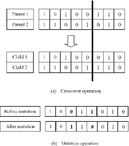
The genetic algorithm (GA) was developed and introduced in 1975 by John Holland [13] as an adaptive learning heuristic. GA is a stochastic search and optimization algorithm based on the theory of natural genetic evolution [14], [15]. GA operates on the population of the candidate solutions which are called chromosomes. Each chromosome is composed of gene bits that represent a set of parameters for the problem. The evolutionary process begins with the initial randomly generated population. Then the population is evolved toward a better solution via genetic operations for many generations. The basic genetic operations are selection, crossover, and mutation. Fig. 1 depicts the simple crossover and mutation operations. In each generation, the selection operation will evaluate chromosomes through the fitness function to select the best ones called parents. The parents are used to produce the new chromosomes called offspring or children by crossover operation. With some low probability, these children are mutated through mutation operation to maintain diversity within the population. The parents and children are grouped together and passed through the survival test. Ones with low fitness value will not survive. This evolutionary process repeats until it meets the termination condition. The population changes over time but its initial size is maintained.
Fig. 1. (a) Crossover operation (b) Mutation operation Recently GA has been used in business, scientific, and engineering problems [14], [16]. Reference [14] applied GA to forecast private sector housing demand in Hong Kong. Ten economic indicators are employed in this study to form the
11-gene chromosomes. One additional gene is the constant term. However, GA models do not provide the good forecasts. One possible reason is that the GA models used all ten indicators which some of them may not be significant. To solve this problem, linear regression analysis (LGA) is applied to select the appropriate indicators. The indicators are selected by the stepwise regression technique. Results from the GA-LGA models are much better than the original GA models. Moreover, the authors also improved the GA-LGA models by using adaptive mutation rate (AMR) approach to reduce the occurrence of local optima. Nevertheless, there is no significant improvement over the GA-LGA models.
The GA is applied to alter the coefficients of the MRA model in this study by SolveXL, the add-in for Microsoft Excel.
C. Neural network
[image:2.595.309.548.338.483.2]The neural network (NN) is originally developed to study the learning process of the human brain [17]. It has an ability to gain the knowledge through learning. The NN may have many structures but the common NN structure is shown in Fig. 2.
Fig. 2. Neural network structure.
This structure consists of three layers, namely input layer, hidden layer, and output layer. Each layer consists of one or more nodes, presented in the figure by circles, which are designed to mimic the neurons or nerve cells. The i, j, and k are the indices of the number of the nodes in the input, hidden, and output layers, respectively. The lines between the nodes represent the information flow between them [17]. The input nodes receive the information from the input variables, x1,x2,…,xn. At the hidden node, the values from the input nodes are multiplied by the weights wij, summed, and then transferred through the nonlinear sigmoid function to the nodes in the succeeding layer. The similar process occurs at the output layer nodes except using the weights wjk. The y1,y2,…,ym are the outputs of the NN. The sample data or training data for NN model are usually divided into three groups – training, validation, and testing [18]. The network is trained by data in the training group. Data in the validation group are used to evaluate the network generalization and halt the training process when the network stops improving. Data in the testing group will provide an independent measure of network performance.
[image:2.595.61.279.455.702.2]construction cost. The data were collected from 71 building construction projects in Gaza Strip, Palestine. Seven variables are used as the input variables of the model including ground floor area, typical floor area, number of storeys, number of columns, type of footing, number of elevators, and number of rooms. The model has one hidden layer with seven nodes and the output layer has one node represented the early stage cost estimation. The results indicate that NN gives reasonable early stage cost estimate.
This research employs the feedforward network, one of the commonly used NN algorithms. This NN model is developed by NeuralTools® from Palisade Decision Tool 5.5.1 software.
III. APPLICATION A. Data
The data used in this study are the construction costs of electrical and communication system collected from 31 industrial factory projects constructed in Thailand between year 2005 and 2011. Twenty five of them are used for training data and the other six are used for testing data. The electrical and communication system is composed of ten sub-systems – high voltage incoming system, substation work system, main feeder for general, power supply for mechanical, lighting and emergency light, telephone system, fire alarm system, public address system, lightning protection system, and outdoor lighting system. In construction cost estimation for industrial factory, one of the key factors is the floor area. In addition, the cost of the electrical and communication system can be classified into five main components which are copper, steel, main equipment, labor, and miscellaneous. Besides, the air condition system is also an important feature of the factory. The construction costs are different between the factories that have and do not have this system. Therefore in this study, the air condition system will be a binary variable which is set to 1 when the air condition system is presented and 0 when it is not.
[image:3.595.304.543.288.496.2]The input and output variables used to developed models are listed in Table I.
TABLE I
LIST OF INPUT AND OUTPUT VARIABLES Variable Symbol Description Input variables x1 Floor area (1,000 m2) x2 Cost percentage from copper x3 Cost percentage from steel x4 Cost percentage from main equipment x5 Cost percentage from labor
x6 Cost percentage from miscellaneous x7 Air condition system
Output variable y Cost of the electrical and
communication system (million baht)
B.Accuracy measurement
The accuracy of each estimation method is measured by the root mean squared error (RMSE) which is defined as:
21
ˆ
n
i i i
y
y
RMSE
n
(2)where
y
iandy
ˆ
i are the observed and estimated costs of the electrical and communication system of the factory i, respectively, and n is the number of data sets.IV. RESULTS AND DISCUSSION A. MRA model
The MRA model determined by Minitab 15 software using all independent variables is:
1 2 3 4 5
6 7
ˆ 28.43 1.39 63.86 2.91 48.49 31.9 8.58 2.943
y x x x x x
x x
(3)
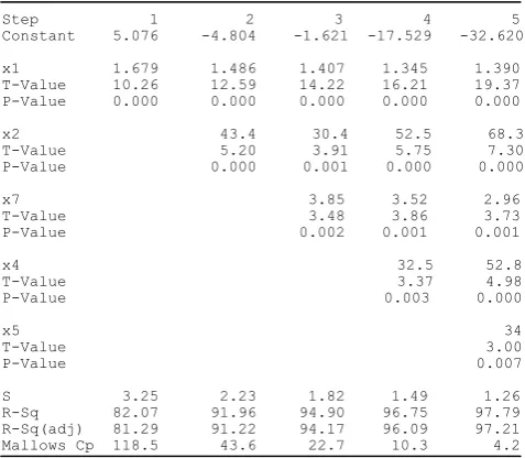
However, some of the parameters have p-values more than 0.05 which indicate that those parameters are insignificant and the corresponding variables should not be presented in the model. Therefore, the stepwise regression function of Minitab 15 software is employed to select the appropriate variables. The result of stepwise regression function is shown in Fig. 3.
[image:3.595.46.291.554.673.2]Step 1 2 3 4 5 Constant 5.076 -4.804 -1.621 -17.529 -32.620 x1 1.679 1.486 1.407 1.345 1.390 T-Value 10.26 12.59 14.22 16.21 19.37 P-Value 0.000 0.000 0.000 0.000 0.000 x2 43.4 30.4 52.5 68.3 T-Value 5.20 3.91 5.75 7.30 P-Value 0.000 0.001 0.000 0.000 x7 3.85 3.52 2.96 T-Value 3.48 3.86 3.73 P-Value 0.002 0.001 0.001 x4 32.5 52.8 T-Value 3.37 4.98 P-Value 0.003 0.000 x5 34 T-Value 3.00 P-Value 0.007 S 3.25 2.23 1.82 1.49 1.26 R-Sq 82.07 91.96 94.90 96.75 97.79 R-Sq(adj) 81.29 91.22 94.17 96.09 97.21 Mallows Cp 118.5 43.6 22.7 10.3 4.2
Fig. 3. Output of stepwise regression function from Minitab 15 software.
The stepwise regression function selects five out of seven variables from the training data (25 data sets) which are floor area (x1), cost percentage from copper (x2), cost percentage from main equipment (x4), cost percentage from labor (x5), and air condition system (x7). The selected MRA model is:
1 2 4 5 7
ˆ 32.62 1.39 68.314 52.83 33.64 2.96
y x x x x x (4)
The R2, adjusted R2, and Cp of this MRA model are 0.9779, 0.9721, and 4.2, respectively.
B. MRA-GA model
TABLE II
LOWER BOUND AND UPPER BOUND OF THE COEFFICIENTS Coefficients Lower bound Upper bound Constant -46.363 -18.877
x1 1.240 1.540
x2 48.738 87.890
x4 30.623 75.037
x5 10.136 57.144
x7 1.300 4.619
GA parameters needed to be specified are the crossover rate and mutation rate. However, the optimum values of these parameters are problem-specific [14]. Therefore, they are determined by trial and error as shown in Fig. 4. The population size and the number of generations are set at 50 and 1,000, respectively. The lowest RMSE is achieved in this experiment when the crossover rate is 0.85 and the mutation rate is 0.15. This results in the MRA-GA model:
1 2 4 5 7
ˆ 32.16 1.409 66.48 52.12 34.68 3.04
y x x x x x (5)
1.09 1.095 1.1 1.105 1.11 1.115 1.12 1.125 1.13 1.135
0.05 0.1 0.15 0.2 0.25 0.3 0.35 0.4
R
MS
E
Mutation rate
0.7 0.75 0.8 0.85 0.9 0.95
Crossover rate
Fig. 4. RMSE of the MRA-GA model with different crossover and mutation rates.
C. NN model
The NN model is developed from 25 sample data sets which are randomly divided into training, validation, and testing groups. In this study, 15 data sets are assigned to the training group. Five data sets go to the validation group and the other five data sets go to the testing group. The input variables are the same as MRA and MRA-GA models. The number of nodes in the hidden layer of the network is determined from the RMSE of the trained network by trial and error as shown in Fig. 5. The network with three hidden layer nodes provides the lowest RMSE so the network in this research is set to have three nodes in the hidden layer.
0.9 0.95 1 1.05 1.1 1.15
2 3 4 5 6 7 8 9 10 11 12 13 14 15 16 17 18 19 20
R
M
S
E
[image:4.595.46.292.87.168.2]Number of nodes
Fig. 5. RMSE of the trained network with different number of hidden layer nodes.
The NeuralTools® also provides the coefficients for the input variables and intercept as shown in Table III. Thus, the NN model can be written as:
1 2 4 5 7
ˆ 33.59 1.426 67.95 55.33 32.37 3.465
[image:4.595.302.550.156.237.2]y x x x x x (6)
TABLE III
INTERCEPT AND COEFFICIENTS FROM NEURALTOOLS® Intercept/Coefficient Intercept -33.590
x1 1.426
x2 67.950
x4 55.330
x5 32.370
x7 3.465
D.Performance comparison
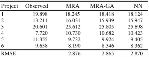
The accuracy of MRA, MRA-GA, and NN models are evaluated and compared in terms of RMSE using six testing data sets. The observed costs, the cost estimates, and RMSEs are shown in Table IV. It can be seen that the MRA-GA model gives slightly lower RMSE than the other two models.
TABLE IV
COST ESTIMATES COMPARISON (MILLION BAHT) Project Observed MRA MRA-GA NN 1 19.898 18.245 18.418 18.124 2 13.211 16.031 15.939 15.947 3 20.601 25.612 25.805 25.698 4 7.720 10.730 10.682 10.423 5 11.355 9.732 9.924 9.405 6 9.658 8.190 8.346 8.362 RMSE 2.876 2.865 2.870
V. CONCLUSIONS
In this paper, three cost estimation methods are used to estimate the costs of electrical and communication system for industrial factory construction. The data used in this study are collected from 31 construction projects in Thailand. Even though in this research, the MRA-GA model delivers the lowest RMSE among three methods, it does not mean that the MRA-GA technique is better than the other two techniques. Since the NN and MRA-GA models take time to develop and the RMSEs are not much different, the MRA model may be more appropriate when the cost estimate is urgently required.
This study estimates the whole system at once. To have a better result, one should estimate each sub-system and then combine to get the cost estimate of the system.
REFERENCES
[1] G.H. Kim, J.E. Yoon, S.H. An, H.H. Cho, and K.I. Kang, “Neural network model incorporating a genetic algorithm in estimating construction cost,” Building and Environment, vol. 39, no.11, pp. 1333-1340, Nov. 2004.
[2] W.D. Yu, C.C. Lai, and W.I. Lee, “A WISE approach to real-time cost estimation,” Automation in Construction, vol. 15, no. 1, pp. 12-19, Jan. 2006.
[3] M.N. Jadid, and M.M. Idrees, “Cost estimation of structural skeleton using an interactive automation algorithm: A conceptual approach,”
[image:4.595.303.552.370.465.2][4] M.Y. Cheng, H.C. Tsai, and W.S. Hsieh, “Web-based conceptual cost estimates for construction projects using Evolutionary Fuzzy Neural Inference Model,” Automation in Construction, vol. 18, no. 2, pp. 164-172, Mar. 2009.
[5] G.H. Kim, S.H. An, and K.I. Kang, “Comparison of construction cost estimating models based on regression analysis, neural networks, and case-based reasoning,” Building and Environment, vol. 39, no. 10, pp. 1235-1242, Oct. 2004.
[6] F.K.T. Cheung and M. Skitmore, “Application of cross validation techniques for modeling construction costs during the very early design stage,” Building and Environment, vol. 41, no. 12, pp.1973-1990, Dec. 2006.
[7] H. Li, Q.P. Shen, and P.E.D. Love, “Cost modeling of office buildings in Hong Kong: An exploratory study,” Facilities, vol. 23, no. 9/10, pp. 438-452, 2005.
[8] T.P. Williams, “Predicting cost for competitively bid construction projects using regression models,” International Journal of Project Management, vol. 21, no. 8, pp. 593-599, Nov. 2003.
[9] M. Gunduz, L.O. Ugur, and E. Ozturk, “Parametric cost estimation system for light rail transit and metro trackworks,” Expert Systems with Applications, vol. 38, no. 3, pp. 2873-2877, Mar 2011.
[10] R.W. Bacon and J.E. Besant-Jones, “Estimating construction costs and schedules: Experience with power generation projects in developing countries,” Energy Policy, vol. 26, no. 4, pp. 317-333, Mar 1998. [11] H.W. Chen and N.B. Chang, “A comparative analysis of methods to
represent uncertainty in estimating the cost of constructing wastewater treatment plants,” Journal of Environmental Management, vol. 65, no. 4, pp. 383-409, Aug. 2002.
[12] C. Stoy, S. Pollalis, and H.R. Schalcher, “Drivers for cost estimating in early design: Case study of residential construction,” Journal of Construction Engineering and Management, vol. 134, no. 1, pp. 32-39, Jan. 2008.
[13] J.H. Holland, Adaptation in Natural and Artificial Systems. Ann Arbor, MI: The University of Michigan Press, 1975.
[14] S.T. Ng, M. Skitmore, and K.F. Wong, “Using genetic algorithms and linear regression analysis for private housing demand forecast,”
Building and Environment, vol. 43, no. 6, pp. 1171-1184, Jun. 2008. [15] L. Sun, X. Cai, and J. Yang, “Genetic algorithm-based optimum
vehicle suspension design using minimum dynamic pavement load as a design criterion,” Journal of Sound and Vibration, vol. 301, no. 1-2, pp. 18-27, Mar. 2007.
[16] D.E. Goldberg, Genetic Algorithms in Search, Optimization, and Machine Learning. Reading, MA: Addison-Wesley, 1989.
[17] S.W. Smith, The Scientist and Engineer’s Guide to Digital Signal Processing. San Diego, CA: California Technical Publishing, 1997, ch. 26, pp. 451-480.
[18] C.M. Bishop, Neural Networks for Pattern Recognition. Oxford: Oxford University Press, 1995.
[19] O. Duran, N. Rodriguez, and L.R. Consalter, “Neural networks for cost estimation of shell and tube heat exchangers,” Expert Systems with Applications, vol. 36, no. 4, pp. 7435-7440, May. 2009.
[20] S. Cavalieri, P. Maccarrone, and R. Pinto, “Parametric vs. neural network models for the estimation of production costs: A case study in the automotive industry,” International Journal of Production Economics, vol. 91, no. 2, pp. 165-177, Sep. 2004.
[21] M.Y. Cheng, H.C. Tsai, and E. Sudjono, “Conceptual cost estimates using evolutionary fuzzy hybrid neural network for projects in construction industry,” Expert Systems with Applications, vol. 37, no. 6, pp. 4224-4231, Jun. 2010.