Abstract—This article is particularly interested in the failure of
a dam and the effects that may induce by the generated failure wave at downstream of the dam. Practical consequences of flooding are hardly a failure if the complete hydraulic calculations of the failure flood are not met. In this optic, different phases of the calculations, involved in the study of rupture of a dam are mentioned. We present and analyze as much as the simple or complex methods can be available to achieve a possible perfect picture of the spread of flood failure. An analysis is presented using available simple or complex methods to achieve, as perfect as possible, a picture of the spread of failure flood.
Index Terms— Boukerdoun dam; unsteady flow; dam failure wave; Saint Venant equation; Discretization; boundary conditions.
I. INTRODUCTION
Floods which are exceptional and natural phenomena are characterized by a sudden rise of water levels and by overflowing rivers. The origin of this rise in water is due to either a rainy episode on the entire basin, or a sudden failure of a dam. This study concerns precisely this type of failure that may lead to waves which behavior as a first step is identical to that of dynamic waves by reducing predominant effect of inertia, then a wave of continuity, as the flooding subsides when moving further downstream. The determination of the propagation of breaking waves should help in providing real-time trends from data recorded at upstream in order to take appropriate protective measures against this phenomenon. The most accurate approach of this phenomenon which requires the least amount of information relating to flooding is based on the numerical modeling of the Saint Venant equations. These equations, which describe the unsteady flow in open channels with free surface, consist of an average description of the depth of flow. As a result of their mathematical complexity, the analytical integration of these equations in the case of an unsteady flow is virtually impossible except in some idealized situations. The presence of projections and hydraulic barriers in transitional flow makes the problem even more difficult. The numerical resolution of the system of partial differential equations (PDE) from
Manuscript received November 09, 2010; revised November 29, 2010. Fourar Ali is Senior Lecturer in the Department of Hydraulics
, Institute of Civil Engineering, Hydraulics and Architecture, Batna University, Algeria (e-mails: afourar7
Lahbari Noureddine is Senior Lecturer in the Department of Hydraulics
Saint-Venant for natural channels can be approached using either the method of characteristics or other methods such as finite differences, finite elements or the finite volume method which is generally preferred for its ability to reproduce digital discontinuous solutions. In this study the finite differences explicit scheme at a fixed time is used, this is a direct method for the solution of the Saint-Venant equations. It is clear that the description of a load of shallow flow does not really fit where the curvature of current lines is significant, which can happen in waves induced by an instantaneous dam failure. For example, the velocity field in the region near the dam is complex, with significant vertical components. But such characteristics are fortunately limited in time and space and their influence on the behavior of distant fields of the flow is relatively low. Properties such as conservation, hyperbolicity, assumption of projections are accepted as obvious properties.
, Institute of Civil Engineering, Hydraulics and Architecture, Batna University, Algeria.
II. DAM FAILURE
A dam failure can be either a total or partial destruction of hydraulic works, their support or their foundations, making them completely ineffective. Hydraulic structures may suffer injury failure more or less seriously. The natural environment is, at one hand, difficult to determine, floods and earthquakes which are random events make difficult to assess their probable extreme intensities on works lifetime. The knowledge and the materials used in the building of works are imperfect, despite the rapid technological advances in the design and implementation of such works in recent decades. The various number of dam failures is (insufficient capacity of the spillway, submersion of the work ...) amounts in thousands of cases since the first works [1] [2]. The most recent data indicate that the number of failures of large dams is on average of about 1.5 per year.
III. FLOW GENERATED BY THE RUPTURE OF A DAM
A. The flood of failure
The most common phenomena associated with failure of concrete structures including as that of Boukerdoun are slipping and overturning for gravity dams and the loss of support or foundation for the arch dam. The failure of a concrete dam causes a displacement as a whole of the structure which inertia limits the development of velocity. The resulting leakage rate is inherent to a process of the opening of the continuous work and partly restricted by the presence of residues of this structure. Whereas, the failure of thin dam looks more like a sudden break releasing instantly a wall of water up to the dam. The flow passing through the dam during the failure may be determined at
Study of an Unsteady Flow at the Downstream
of a Hydraulic Structure and its Influence on the
Streambed
any time if the shape of the hole is known. Therefore, calculations by formulas of a general hydraulic hydrograph resulting from the flood of rupture depends on the available knowledge on such phenomena as earthquakes, floods or other multiple forms of development and characteristics of materials used ( strength, consistency, implementation, local
damage). Using data derived from the failures observed in the past, the magnitude of the flows resulting from these
failures can be roughly estimated[3].
B. Predetermination of maximum probable flow through the structure
To determine the maximum possible flow of failure of Boukerdoun dam, the relationship Ritter [4] is used, assuming an instantaneous failure. This relationship gives a first estimation of the maximum flow in the gap:
5 . 1 0 2 max 0.9 LH
Q = (1) where: the constant-width of the dam making way for the
flood, (m) - initial depth of water upstream
C. Forecast of the failure wave propagation at downstream of the dam [5][6]
Among the techniques for predicting the propagation of failure waves in the flow, in-situ tests or on reduced model, the theoretical and numerical models, given the rivers, objectives and informations available, can be mentioned Mathematical models, also constantly developed and improved, are used today.The current situation highlights the importance of numerical models in studies of failure flood propagation of their ability to take into account the mode of failure of structure, the geometry of the channel, effluents, and the boundary conditions has made them compulsory in all studies of dam’s failure. However, it should be clear that the choice of calculation methods is an important step to get the desired results and the choice must take into account the specific characteristics of each work. The values of parameters used to define the gap have a large effect on fracture rates and flooding generated near the dam. As the distance from the hole and the wave progresses downstream these values decrease and their influence becomes negligible [7].
IV. MODELS FOR CALCULATING THE PROPAGATION OF THE FAILURE WAVE Nowadays the use of dimensional models is the most common because it meets the needs of the vast majority of studies undertaken. Whereas the two-dimensional models can complete, elaborate or qualify certain aspects treated in a comprehensive manner by the assumptions of the unidimensional approach. In other situations, the combination of both models is the ideal tool for analysis, provided of course the knowing of advantages and limitations of each.
A. Setting equation for the phenomenon of failure and flood wave propagation
Flood dam failures are free surface flows, non permanent, and non-uniform with horizontal main components [8]. The dynamic equations describe their change and their transformation through the various sections of the canal. The formulation of Saint-Venant is written in
the form of a system of two equations, one representing the conservation of fluid mass, the other, the conservation of its momentum. These conservations imply a vertical distribution of hydrostatic pressure, zero vertical velocity and low vertical accelerations. Their validity is limited to relatively slow variations in space and time. Calculated local velocities are horizontal and represent an estimate on the average depth. By neglecting the transverse velocity relative to the longitudinal velocity and the differences in transversal water level, these equations integrated over the transversal dimension will be reduced to a unidimensional form. The one-dimensional shape calculation means in practice a further simplification of the data calculation. The spread of the flow is along the channel.
B. Equation of mass conservation with free surface [6],[7]and[8]
For an incompressible liquid and a supposed one-dimensional flow, the equation of conservation of mass is:
( )
x q t S x Q= ∂ ∂ + ∂ ∂
(2) The function represents the lateral flow per unit length of the curvilinear abscissa of the channel. Considering the particular derivative of the volume occupied within a control surface, the equations are written as follows:
( )
∫
∫∫
⋅ == 2
1
x x
SV ndS q x dx
Dt
Dv
(3) On the free surface Vn
( ) ( )
∫
=∫
( )
∂ ∂ +
− 2
1
2 1 ,
, 1
2
x x
x x qxdx
dx t y B t x Q t x Q
=∂y / ∂t since y(x, t) is the draught. The flow is still one-dimensional, the element of the surface d s of the free surface is written d s = B d x since B(x, t) represents the mirrored image of the width of the wet cross section at abscissa x and at time t. The balance of flow is:
(4) where:
(
)
(
)
∫
∂ ∂ =
− 2
1 ,
, 1
2
x
x x dx
Q t
x Q t x
Q (5)
The environment is assumed continuous, the theorem of the zero integral leads to the equation:
( )
x q t y B x Q= ∂ ∂ + ∂ ∂
(6) Note that B d y represents the increase in the wet section at the curvilinear abscissa x. The previous equation becomes:
( )
x q t S xQ =
∂ ∂ + ∂ ∂
(7)
C. Different forms of the equation of conservation of mass [7],[9]:
C.1. Taking into account the velocity
The equation of conservation of mass, taking into account the relation (2), is written as:
( )
x q t S x U S x SU =
∂ ∂ + ∂ ∂ + ∂ ∂
(8)
C.2. Taking into account y and B
B
q
t
y
x
U
B
S
x
y
U
=
∂
∂
+
∂
∂
+
∂
∂
(9)C.3. Taking into account the speed of the wave
The ratio is by definition the average draught. By replacing, the equation of conservation of mass for a prismatic channel
is obtained:
B
q
t
y
x
U
g
c
x
y
U
=
∂
∂
+
∂
∂
+
∂
∂
2 (10) The general equation of conservation of mass is written below:( )
x q t S x U S x S U = ∂ ∂ + ∂ ∂ + ∂ ∂ (11)D. Saint Venant equation for free surface
The equation of Saint-Venant for prismatic channel and without any side is given by:
0 2
1 2 − + =
∂ ∂ + ∂ ∂ + ∂ ∂ J J g U x x y t U
g f (12)
D.1. Introduction of flow instead of speed in Saint Venant equation
Since the flow is unidimensional and considering the equation
Q
=
SU
, the general equation of conservation of mass, taking into account any side input is written:q
x
Q
x
S
=
∂
∂
+
∂
∂
(13) The termt
U
g
∂
∂
1
, reflecting the unsteadiness of the flow, when taking into account the equation of conservation of mass is written:
x Q gS Q gS Qq t Q gS t U g ∂ ∂ + − ∂ ∂ = ∂ ∂ 2 2 1 1 (14) The term
x
H
∂
∂
, if
α
=
1
is to be written:x S gS Q x Q gS Q x y J x H f ∂ ∂ − ∂ ∂ + ∂ ∂ + − = ∂ ∂ 3 2
2 (15)
The Saint Venant equation takes the following form, by combining some terms:
∂y/∂x(1-Q2L/gS2)-Jf+J+1/gS ∂Q/∂t- Qq/gS2 +2Q/gS2∂Q/∂
x-Q2/gS3(∂S/∂x)y,t= -1/S[∂(hGS/∂x ] y,t
0
1
=
∂
∂
t
Q
gS
+qV/gS(16) Since the flow is permanent , the draught and The speed are function of the abscissa
x
of the flow. The channel is prismatic, and the terms:0 , 3 2 = ∂ ∂ − t y x S gS Q
and 1
(
)
0, = ∂ ∂ − t y G x S h S
The flow is gradually growing in the channel, thus
q
dx
dQ
=
the previous equation becomes:
gS qV gS Qq J J gS L Q dx dy
f + + =
− − 2 3 2
1 (17)
V. NUMERICAL METHOD OF RESOLUTION OF THE SAINT VENANT SYSTEM
A. Discretization of the domain
Solving the problem of dam failure is possible through the use of the following one-dimensional Saint-Venant equations:
(
)
− = ∂ ∂ + ∂ ∂ + ∂ ∂ = ∂ ∂ + ∂ ∂ + ∂ ∂ J J g x y g x U U t U x U y x y U t y f 0 (18)Where y is the height of water, Ū, represents the average velocity of flow. Each of the two quantities depends on time t and space x. By replacing the governing partial differential equations by finite differences the resulting algebraic equations at each point of the network or at each node can be solved, by assuming the initial values at time to the speed and the flow depth at all points of this network. At to
x
t
∆
∆
+ Δt the following values corresponding to this interval of time are determined Several explicit schemes have been used for the unsteady flow with a free surface of which the diffusive Lax scheme is taken for the fact that it is a numerically stable condition according to the value of the dimensionless parameter Cr = u ≤1,0. In this scheme, the governing partial differential equations are replaced by finite difference quotients as follows:
t y y t y i j i ∆ − = ∂
∂ +1 *
(19) t U U t U i j i ∆ − = ∂
∂ +1 *
(20)
x U U x
U ij ij ∆ − = ∂ ∂ + − 2 1 1 (21) Where:
(
j)
i j i
i y y
y*=0.5 −1+ +1 (22)
(
j)
i j i
i U U
U* =0.5 −1+ +1 (23)
B. Discretization in space
equations are discretized with a centered scheme:
x U U y x y y U t
y i i
i i i i ∆ − − ∆ − − = ∂ ∂ + − + − 2 2 1 1 1 1 (24)
(
f i)
i i i i i
i gJ J
x y y g x U U U t U − + ∆ − − ∆ − − = ∂ ∂ + − + − 2 2 1 1 1 1 (25) for a variable, a; ai = a (xi) where xi
This equation is applicable only to nodes that are not at the edges, but as in any problem the limitations on the edges are known so the Riemann problem can be solved. In addition:
= i. Δx
( )
2 3 4 n Rh U U J i i ii = (26) Where:
n
- Manning coefficientC. Discretization in time
evaluate ∆ − − ∆ − − ∆ + = + − + − + x U U y x y y U t y y j i j i j i j i j i j i i j i 2 2 1 1 1 1 * 1 (27)
(
)
− + ∆ − − ∆ − − ∆ + = + − + − ++1 * 1 1 1 1 1
2 2 j i f j i j i j i j i j i i j
i gJ J
x y y g x U U U t U
U (28)
( )
2 1 3 4 1 1 1 ) ( n Rh U U J j i j i j i j i + + + + = (29) By putting:( )
(
)
g
t
Rh
n
j i∆
=
Γ
− +1 3 4
2 1
and multiplying the
equation (28) by
Γ
−1, the following equation is obtained:[ ] [ ]
Uij+12+ΓUij+1−Γβ
=0 (30) where: ∆ + ∆ − ∆ ∆ − ∆ − ∆ ∆ −= + − + − f
j i j i j i j i j i
i g tJ
x y y x t g x U U U x t U 2 2 2 2 1 1 1 1 *
β
This is a quadratic equation in
U
ij+1 and it follows that:(
)
Γ + Γ + Γ − =+1 2 21
4 2
1
β
j i
U (31)
D. Conditions at upstream limit
At the upstream limit it is accepted that
x
y
y
x
y
ijj i
∆
−
=
∂
∂
+1, so the equation (27), of which the depth is modified and contains only terms with indices i and i +1,becomes:
(
) (
)
[
j]
i j i j i j i j i j i j i j
i U y y y U U
x t y
y +1 − +1 + − +1 ∆
∆ +
= (32)
The speed can be then obtained with
1 1 1 + + + = j i j i j i S Q
U ,where: Sij+1 - wet surface corresponding
to the depth
h
ij+1E. Conditions at downstream limit
For the downstream end of the channel, the situation is the opposite of that of the upstream.
Assuming that:
x
y
y
x
y
i i∆
−
=
∂
∂
−1the equation (26), of which the depth is modified and containing only terms with the indexes
i
andi
−
1
, is written as follows:(
) (
)
[
j]
i j i j i j i j i j i j i j
i U y y y U U
x t y
y − + −
∆ ∆ + = − − + 1 1 1 (33)
F. Stability of the scheme
It is usually required in explicit finite difference schemes that the ratio of Δx and Δt satisfies a condition of stability. A scheme is stable if an error made in the solution does not increase when the calculations are progressing in time. In the case of unstable scheme the error is amplified quickly and masks the true solution in some time intervals. In order
that Lax scheme should be stable, the time and space steps must meet the following condition, called condition of stability of flow:
c
U
x
t
+
∆
≤
∆
(34)VI. NUMERICAL RESULTS
During a dam failure, a wave propagates downstream along the channel leading to significant flooding. The calculation program (dam failure) that is developed in Delphi aims to give an order of magnitude of the respective levels achieved in such a channel. The information provided in this program (dam failure) are the height of water in the dam and the width of the latter, the length, slope and roughness of the channel which allow to estimate the flow, the speed, the height and also the speed of the wave at different points in the channel that the user can choose to get results. This program is suitable for instant failures. The user must provide the maximum flow at the dam. In this case the Ritter formula (1) is used for the estimation of the maximum failure flow for rectangular shape of the gap failure.
In a given channel, the program performs the following calculations:
- Calculation of inflow at the dam with a hydrograph of failure flow
- Calculation of reached water level at the foot of the dam using the equation (32), then the speed through the hypothesis of the uniform state and finally the speed. - Calculation of the water level reached at the downstream end of the channel through the equation (33), then speed through the uniform state hypothesis then the flow and the speed.
- Calculation of the water level and the speed reached in the intermediate nodes of the channel by the equation (27) and (31), then the flow and the speed of the waves caused by the failure.
- The results are highly dependent on assumptions considered in the choice of different parameters (Manning coefficient, slope, height of initial water in the dam, width of the dam ....). In this context, a low reading can only come from repeated use of the program in a same problem. It should also be noted that some cases are, a priori, excluded, such as:
The presence of singularities (topography or work irregularity) very marked.
A. Dam Characteristics
Maximum height of the dam: 55.0 m, crest length 609.7 m, crest width 10 m. The maximum level of natural terrain 367.62 m. The length of the channel is equal to 14737.29 m, the channel slope equals to 0.001, and Manning’s coefficient equals to 0.05.
The maximum flow at the time of failure, which depends on the geometry of the dam, and obtained by the Ritter formula, is: Qmax = 0.81*609.7*553/2 m3
In view of the results obtained by simulation by means of the calculation program developed in Delphi, the Boukerdoun dam may constitute, upon failure, a real danger for all the infrastructure of any kind whatsoever and for
/s.
people who located downstream of the dam. The most precise approach to the problem, requiring less data on the flood, is that of the numerical modeling of St Venant equations. In these equations, the unknown is the speed and the height of water, and to perform the mathematical modeling, the studied channel is cut in several sections, and with the numerical scheme used, in this case, the finite difference method, the partial derivatives are replaced by an algebraic system that has allowed to calculate approximate values of velocities and water heights.
In this study, relative to an instantaneous failure, and as illustrated by the figures above namely those of heights, speeds and flow rates (Figures 1 to 10) and also the speed of the waves and taking into account the variation of the slope, the roughness of the walls and filling heights inducing dynamic variables at time t = 1390.1 s and at the foot of the dam, the downstream area is suddenly submerged. The water depth and the flow reach respective values of 39.2136 and 190808.2 m m3 / s, the speed is about 7980 m / s, the speed of the wave reaches a value of 19.6134 m / s, reflecting the very violent feature (Fr =
c
U
≈ 2.0) of the
flow which impacts on the shape of the channel are very irreversibly devastating. At a distance x = 7368.645 m and time always equals to 1590.1 s, a very sharp increase in flows and speeds at the expense of a reduced height of approximately 13.63031 m is observed. This decrease is explained by the effect of wall friction which caused a loss of relatively large load. Finally at t = 3.47 hours and at a distance of x = 14737.29.0 m all hydraulic parameters of flow cancel out by virtue of the power loss of hydraulic flow. Water levels calculated at all points downstream of the dam depend particularly on the resistance factor used, namely the Manning coefficient n to characterize the active bed of the channel (Fig. 6, 7). More the resistance to flow and the loss of linear and local loads are important more the speed of propagation of the flood decreases resulting therefore in a higher flood and greater erosion. It should be noted that the results obtained by simulation are dependent on the boundary condition used at the edge
max
Q
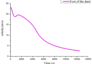
of the failure area given by the Ritter formula. The simulations carried out on the flow generated by a hypothetical failure of the Boukerdoune dam, and given their dynamic energy suggest that the spread of the resulting flooding is always accompanied by a quarrying and a major transfer of major sediments in some parts of the downstream channel causing significant physical changes in the geometry of the channel. In areas with low or zero slopes therefore suitable to the deposit of over thrust material because the hydraulic power decreases, the maximum water levels observed and calculated are due especially to the raising of the bottom of the channel. The stability and safety of hydraulic structures and the behavior of the dams are heavily dependent on the calculation of the failure wave propagation downstream of these structures. For the initially retained scheme, ie an instantaneous failure, it allows to draw a hydraulic picture of the failure floods that the work might generate. This scheme has provided a large amount of informations, concerning the unsteady flow, calculated at several points in the downstream channel of the Boukerdoune dam. The duration of the simulations can be hours if it is desired to reach the emptying of the reservoir to [image:5.595.346.504.129.239.2]find when the water has returned to normality, at least in appearance. Failure waves as indicated by the (fig. 1, 4) diminish gradually moving up to the downstream of the dam, ie the distance x = 2653 m, up to time t = 2000s reaching the maximum value of 35m to extinguish off completely at the end of the term at x = 12379 m.
[image:5.595.336.516.268.504.2]Fig.1. Variation of the wave velocity of failure at the foot of the dam.
Fig. 2. Variation of the height at x =7368.645 m of the dam
[image:5.595.335.518.530.646.2].Fig. 3. Variation of the velocity at x = 7368.645 m of the dam.
Fig. 4. Variation of the wave velocity of failure at x = 7368.645 m
[image:5.595.338.523.665.773.2]Fig.6. Influence of Manning coefficient on the velocity(x=7368.645 m).
Fig.7. Influence of Manning coefficient on the velocity(x = 7368.645 m).
Fig.8. Influence of slope thewater level (x = 7368.645 m).
Fig.9. Influence of slope on the velocity (x = 7368.645 m).
Fig.10. Influence of slope on the velocity (x = 7368.645m).
VII. CONCLUSION
Failure studies are fundamental elements of the safety analysis of a dam. They provide a fairly accurate picture of runoff that must be propagated to downstream areas receiving flood failure waves and the time should make this wave to reach the areas where flooding could result in very damaging consequences. They aim to enable the conception of protecting works such embankment, recalibration, and respecting up in such a way that floods generated by the rupture do not affect the geometry of the channel through their erosive effects and the organization of emergency to protect people and property against flooding. Often, failure studies give the possibility to collect data covering the reservoir and it’s downstream. The data relating to the topography and bathymetry are often used by numerical models. As a reliable source that transmits the various codes of calculation of reliable data and consistent with the degree of precision required by the calculations, these data are used to perform the calculations of the Boukerdoune dam. In themselves, these calculations are now simple and inexpensive to run. The results of failure are very useful for the safety of structures. They should therefore be exploited in an optimal way to secure a maximum of these works against floods which can cause their destruction. The security of coastal populations depends on the quality of information they receive. It is necessary to interpret the numerical results or graphs such as those presented in this study and to convey avoiding any ambiguity, but taking into account the limitations inherent in scientific studies.
REFERENCES
[1] A.Goubet, analyse des ruptures de barrages, causes et conséquences, sécurité des barrages en service, engref, 1993
[2] V. P. Singh dam break modeling technology, Dordrecht, Kluwer Academic Publishers, 1996.
[3] J. E. Costa, floods from Dam Failures, Rapport 85 -560, Denver, USGS, 1985; icold, étude d’onde de rupture de barrage, Synthèse et recommandations, Paris, Commission internationale des Grands Barrages, 1998.
[4] A.Goubet, analyse des ruptures de barrages, causes et conséquences, sécurité des barrages en service, engref, 1993
[5] V. P. Singh dam break modeling technology, Dordrecht, Kluwer Academic Publishers, 1996.
[6] J. E. Costa, floods from Dam Failures, Rapport 85 -560, Denver, USGS, 1985; icold, étude d’onde de rupture de barrage, Synthèse et recommandations, Paris, Commission internationale des Grands Barrages, 1998.
[7] Stoker J. J., water waves, New York, Intersciences Publishers Inc, 1957.
[8] zerrouk E.D.,C.Marche, les prevision des brèches de rupture des barrages en terre restent difficiles, revue canadienne de génie civil, vol 28, 2001.
[9] Wahl T., Prediction of Embankment Dam Breach Parameters, a Literature review and Needs Assessment, rapport DSO-98-004, Denver, dam Safety office, Water Resources Research Laboratory, US bureau of Reclamation, 1998.
[10] D. L. Fread, some limitations of dam breach flood routing models, ASCE Fall Conversion, St, Louis, ASCE, 1981.
[11] Cunge J.F. et al: Practical aspect of computational River Hydraulics. Pitman. Ltd, London. GB, 1980
[12] Abbot M.B et Basco D.: Computational fluid dynamics. Longman Sci. and Techn., Harlow, GB, 1989.