An environmental input?output model for Ireland

An Environmental Input–Output

Model for Ireland

JOE O’DOHERTY

The Economic and Social Research Institute, Dublin

RICHARD S. J. TOL*

The Economic and Social Research Institute, Dublin

Institute for Environmental Studies, Vrije Universiteit, Amsterdam, Carnegie Mellon University, Pittsburgh, PA

Abstract: This paper is presented in two parts. The first part demonstrates an environmental

input-output model for Ireland for the year 2000. Selected emissions are given a monetary value on the basis of benefit-transfer. This modelling procedure reveals that certain sectors pollute more than others – even when normalised by the sectoral value added. Mining, agriculture, metal production and construction stand out as the dirtiest industries. On average, however, each sector adds more value than it does environmental damage. The second part uses the results of this input-output model – as well as historical data – to forecast emissions, waste and water use out to 2020. The growth in emissions of fluorinated gases and carbon monoxide and the growth of hazardous industrial waste exceed economic growth. Other emissions grow more slowly than the economy. Emissions of acid rain gases (SO₂, NO_xand NH₃) will decrease, even if the economy grows rapidly.

157

*John Fitz Gerald, Sean Lyons, Sue Scott and an anonymous referee had valuable comments on earlier versions of this paper. Adele Bergin, Yvonne McCarthy and Sue Scott pointed us to crucial data. The Environmental Protection Agency provided welcome financial support.

I INTRODUCTION

W

ith rapid economic growth comes rapidly growing pressure on the environment, while concern about pollution and resource use waxes too. Ireland is no exception. Although it has leapt forward to become one of the richest countries on the planet, its environmental care is more typical of a middle-income country. As improving the quality of life depends less on increasing economic wealth, the people of Ireland will reprioritise and seek a new balance between the economy and the environment.

Efforts elsewhere to develop a balance between economic and environmental objectives have required complex modelling of national, regional, or even world economies and their interaction with the environment (see Duchin and Lange, 1994; Dellink et al., 1999). In an Irish context, the imperatives implied by the Kyoto Protocol and the Water Framework Directive1 _{will require the construction of similar models so as to develop a} thorough understanding of environment-economy linkages and the effect of policy.

Like environmental care, research in environmental economics is underdeveloped in Ireland. This paper makes a modest step forward by introducing a preliminary environmental input-output model (EIO). EIOs are a suitable tool for estimating the short-term response of emissions and resource use to changes in consumption and production, be it induced by economic growth or by changes in (environmental) policy. Like input-output models, EIOs are static and linear. The data needed for constructing an EIO are a subset of the data needed for a more dynamic environment-economy model for the medium term. An EIO is, therefore, a useful first step – and, with proper caveats, can yield policy insights too.

According to its founder, Wassily Leontief,

… input-output analysis describes and explains the level of input of each

sector of a given national economy in terms of its relationships to the

corresponding levels of activities in all the other sectors(1970, pp. 262).

Essentially, this involves a matrix representation of the economy in order to predict the effect of changes in one industry on others, while at the same time modelling the effect of this interaction on consumers, the government and foreign suppliers.

1 _{Directive 2000/60/EC of the European Parliament and of the Council of 23 October, 2000}

The first effort to model the effect of these interactions on the environment was undertaken by Leontief himself, when in 1970 he sought to account for pollution and a new industry aggregation – the anti-pollution industry – within a hypothesised two-sector, two-good economy.

However, Van den Bergh and Hofkes (1999, p. 1114) note that “… the most important recent study [in environmental input-output modelling] is by Duchin and Lange (1994)”. Their ambitious model involves a detailed input-output model of the world economy, covering the dynamics of trade in sixteen regions and fifty sectors. This study sought to test the Brundtland Commission’s statement that growth and sustainable development could go hand in hand, and concluded that this is not the case.2

A common issue in relation to input-output models is that these models “… are structurally fixed in the sense that sectoral classification and disaggregation, and assumed technologies, cannot change endogenously” (van den Bergh and Hofkes, 1999, p. 1115).

One effort to overcome these problems is the Regional and Welsh Appraisal of Resource Productivity and Development (REWARD) project in the UK (see Ravetz, et al., 2003). The project distinguishes different regions of the UK and thus further subdivides the standard input-output modelling framework to create a Regional Economy-Environment Input-Output (REEIO) model. Environmental input-output modelling is furthest developed in the USA. The EIOLCA model (www.eiolca.net; Hendrickson et al., 2006) has almost 500 economic sectors and a long list of resources and emissions. Such data are unfortunately not available for Ireland.

The model presented in this paper is ISus 0.0, the prototype for Ireland’s Sustainable Development Model. ISus 0.0 is an input-output model comprising 19 sectors, 13 pollutants, five classifications of waste, and water use. It is constructed such that it models the production side of the Irish economy. Household demand is included, but household pollution is not, although its contribution is substantial (see Barrett et al., 2005, p. 83). Household demandis, of course, included. The model as presented here is able to address the following questions: Which sectors of the economy produce the largest quantities of pollutants? Which sectors add the most value – considering the environmental damage they cause? How is the situation likely to change in the future?

2_{Dellink et al.(1999) extend a computable general equilibrium model to environment-economy}

There is a large body of research on the relationship between economic and social activity and key environmental media in Ireland,3 _{though until now} these analyses have employed medium-term econometric models, rather than input-output models as we do here.

The paper is presented as follows. Section II reviews the structure of environmental input-output models. Section III discusses the data and the basic results. Section IV presents environmental efficiencies and compares them to damage cost estimates from existing research. Section V presents forecasts of emissions and intensities out to 2020. Section VI concludes.

II INPUT-OUTPUT AND ENVIRONMENTAL INPUT-OUTPUT MODELS

Goods and services are produced either for consumption or for use in further production. That is,

X₁= X_1,1+ X_1,2+ … + X_1,n+ Y₁

X₂= X_2,1+ X_2,2+ … + X_2,n+ Y₂

(1) …

X_n= X_n,1+ X_n,2+ … + X_n,n+ Y_n

where X_i is the production of good i, and X_i,j is the use of good i in the production of good j; Y_i is the consumption of good i, which, for convenience, includes exports and build-up of inventories. Equation (1) can be rewritten as

X₁= a_1,1X₁+ a_1,2X₂+ … +a_1,nX_n+ Y₁

X₂= a_2,1X₁+ a_2,2X₂+ … +a_2,nX_n+ Y₂

(2) …

X₂= a_n,1X₁+ a_n,2X₂+ … +a_n,nX_n+ Y_n

3_{The relationship between greenhouse gas emissions and the economy has been modelled by}

Conniffe et al.(1997), Bergin et al.(2003) and Fitz Gerald (2004). Teagasc has modelled the impact of agriculture on greenhouse gas emissions (Behan and McQuinn, 2002). Work on the impact of economic activity on the generation of solid waste is described by Barrett and Lawlor (1995). The state of research on the link between economic activity on water use and emissions to water is described by Scott (see Scott et al., 2001 and Scott, 2004). Finally, a range of different types of research on transport has been carried out for Ireland (see Department of Public Enterprise, 2000), and a simplified model of the transport sector is already incorporated into the ESRI’s

where

X_i,j

a_i,j: = –— (3)

X_i

In matrix notation,

X₁ = a_1,1 a_1,2 … a_1,n X₁ Y₁

X₂ = a_2,1 a_2,2 … a_2,n X₂ Y₂

= + (2') … … … … … … …

X_n = a_n,1 a_n,2 … a_n,n X_n Y_n

or

X = AX + Y ⇔ (I – A)X = Y ⇔ X = (I – A)–1_{Y= LY (2")}

Equation (2) specifies how production X would respond to a change in demand Y, including all intermediate production. Lis commonly referred to as the Leontief inverse.

Emissions Mof substance lequal

M_I= b_i,1X₁+ b_i,2X₂+ … b_i,nXn᭙l (4)

where b_l,iare the emission coefficients, that is, emission per unit of production. In matrix notation,

M= BX= BLY (5)

Equation (5) relates emissions to production (via B) and to final consumption (via BL).

III DATA

CSO (2006a) has the input-output tables for Ireland for 2000 for 48 sectors according to NACE.4_{CSO (2006b) has the environmental accounts for Ireland} for 1997-2004 for 19 sectors, which are aggregates of NACE sectors. Data are

⎤ ⎪ ⎪ ⎪ ⎪ ⎪ ⎪

⎦ _⎤

⎪ ⎪ ⎪ ⎪ ⎪ ⎪

⎦ ⎤

⎪ ⎪ ⎪ ⎪ ⎪ ⎪

⎦ _⎤

⎪ ⎪ ⎪ ⎪ ⎪ ⎪ ⎦ ⎤

⎪ ⎪ ⎪ ⎪ ⎪ ⎪

⎦ _⎤

⎪ ⎪ ⎪ ⎪ ⎪ ⎪ ⎦

⎤ ⎪ ⎪ ⎪ ⎪ ⎪ ⎪

⎦ _⎤

⎪ ⎪ ⎪ ⎪ ⎪ ⎪ ⎦

4_{NACE is a statistical classification of economic activities. NACE is an acronym for}

limited to the main greenhouse and acidifying gases. EPA (2005a) has data on carbon monoxide, volatile organic compounds, hydrofluorocarbons (‘HFCs’; 13, of which 8 have zero emissions) and fluorinated gases (‘F-gases’; 8, of which 4 have zero emissions). We aggregated the HFCs and F-gases based on their 100-year global warming potential (Ramaswamy et al., 2001). Scott (1999) presents data for solid waste and eutrophication, for the same 19 sectors, for 1994. According to Toner et al. (2005), eutrophication has hardly changed between 1994 and 2000, so we used Scott’s 1994 data for 2000. EPA (2005b) has sectoral data on waste for 2004. We interpolated between 1994 and 2004 to get ‘data’ for 2000. Camp Dresser and McKee (2004) report abstractive water use per sector, for 2001 for selected industrial sectors and for an unknown year for agriculture. We assume that these data hold for 2000.

We aggregated the 48 sector output table to the 19 sector input-output table, computed the Leontief inverse (L), the emission coefficients of production (B), and the emission coefficients of consumption (BL) for carbon dioxide (CO₂), nitrous oxide (N₂O), methane (CH₄), sulphur dioxide (SO₂), CFCs and F-gases (CFC+F), carbon monoxide (CO), volatile organic compounds excluding methane (VOC), nitrogen oxides (NO_x), ammonia (NH₃), agricultural waste, industrial waste (hazardous or not, recycled or not), organic matter (BOD), nitrogen (N), phosphorus (P), and water (H₂O).

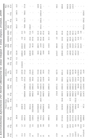
Table 1 shows the 2000 emissions, waste and water use per sector, and the sector’s economic output. Tables 2 and 3 show the emission coefficients of production, measured by total output and by value added, respectively. Table 4 shows the emission coefficients of consumption. These tables contain no qualitative surprises, at least to those who have studied environmental pollution, but the numbers are interesting nevertheless. Table 1 shows that whereas economic activity is concentrated in services, pollution is mostly from agriculture, industry and transport. Tables 2 and 3 confirm this, with low emission coefficients for services, but higher ones for the other sectors.

[image:7.556.72.421.87.625.2]

T

able 1:

Emissions, W

aste and Consumptive W

ater Use, Per Economic Sector and Supply at Basic Prices, Ireland,

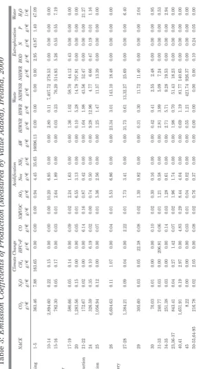
2000 Climate Change Acidification W aste Eutrophication W ater Economy NACE CO 2 N2 OC H4 HFC+F C O NMVOC SO 2 No x NH 3 A W HIWNR HIWR NHIWNR NHIWR BOD N P H2 O Supply 10^9 g 10^9 g 10^9 g 10^9 g 10^9 g 10^9 g 10^9 g 10^9 g 10^9 g 10^9 g 10^9 g 10^9 g 10^9 g 10^9 g 10^9 g 10^9 g 10^9 g 10^6 l 10^6 € Agriculture, forestry , fishing 1-5 1,230.3 26.7 554.0 0.0 0.0 0.0 3.2 15.1 120.7 56,516.2 0.0 0.0 0.0 0.0 10.0 148.5 4.7 159,405 6,945

Coal, peat, petroleum,

metal ores, quarrying

10-14 1,005.8 0 .1 0.1 0.0 0.0 0.0 3.5 2.4 0.0 0.0 1.0 0.0 2,573.9 96.8 0.0 0.0 0.0 0 1,481

Food, beverage, tobacco

15-16 2,579.6 0 .2 0.5 0.0 0.1 0.0 8.7 6.2 0.0 0.0 0.1 0.8 251.3 1,698.0 17.3 1.8 1.8 23,721 13,696 T

extiles Clothing Leather & Footwear

17-19 243.1 0.0 0 .1 0.0 0.0 0.0 0.9 0.7 0.0 0.0 0.6 0.4 24.6 18.5 0.2 0.0 0.0 0 3,219 W

ood & wood products

20 269.7 0.0 0 .0 0.0 0.0 0.0 1.4 0.7 0.0 0.0 0.0 1.1 3.1 167.7 0.0 0.0 0.0 0 956

Pulp, paper & print

production 21-22 251.1 0.0 0 .0 0.0 8.9 0.2 1.3 0.6 0.0 0.0 2.4 2.9 63.3 76.3 0.0 0.0 0.0 30,930 7,732 Chemical production 24 2,563.0 2 .7 0.8 48.6 0.1 0.0 5.8 3.9 0.0 0.0 72.8 101.7 37.4 52.3 3.7 1.5 0.1 9,082 22,285

Rubber & plastic

production 25 356.9 0.0 0 .0 0.0 0.0 0.0 1.8 0.9 0.0 0.0 0.4 0.5 3.8 4.5 0.0 0.0 0.0 0 2,069 Non-metallic mineral production 26 3,122.1 0 .1 0.5 0.0 0.0 0.0 2.6 3.2 0.0 0.0 11.0 1.4 67.6 8.7 0.0 0.0 0.0 0 1,633

Metal prod. excl. machinery

& transport equip.

27-28 760.9 0.0 0 .0 0.0 1.2 0.0 4.2 1.9 0.0 0.0 17.4 0.3 732.4 14.1 0.0 0.0 0.0 3,520 3,331

Agriculture & industrial

machinery 29 190.5 0.0 0 .0 14.0 0.1 0.0 0.8 0.5 0.0 0.0 0.2 0.2 7.3 7.1 0.0 0.0 0.0 1,275 4,716

Office and data process

machines 30 165.7 0.0 0 .0 0.0 0.2 0.0 0.7 0.4 0.0 0.0 1.0 1.0 6.0 5.9 0.0 0.0 0.0 2,256 20,861 Electrical goods 31-33 716.0 0.1 0 .0 615.0 0.2 0.0 3.6 1.7 0.0 0.0 8.3 11.9 15.1 21.5 0.0 0.0 0.0 1,577 14,589 T ransport equipment 34-35 99.1 0.0 0 .0 0.0 0.1 0.0 0.5 0.2 0.0 0.0 1.1 2.3 3.7 7.7 0.0 0.0 0.0 1,160 4,775 Other manufacturing 23,36-37 398.2 0.0 0 .1 0.7 0.0 0.0 0.9 0.8 0.0 0.0 0.9 0.3 24.3 8.6 0.0 0.0 0.0 0 2,506 Fuel, power , water 40,41 1,396.0 0 .2 2.5 0.0 4.1 0.2 7.1 3.4 0.0 0.0 0.6 1.0 69.1 118.9 0.0 0.0 0.0 0 2,365 Construction 45 44.9 0.0 0 .0 0.0 0.2 0.0 0.2 0.1 0.0 0.0 3.0 6.6 2,304.8 5 ,062.7 0.0 0.0 0.0 0 15,517

Services, excl. transport

50-55,64-95 7,733.5 0 .9 73.0 0.0 2.9 0.6 27.2 13.3 0.0 0.0 0.0 0.0 0.0 0.0 3.6 8.5 1.8 0 70,629 T ransport 60-63 11 ,062.4 1 .2 2.6 0.0 178.2 25.1 3.5 60.9 1.8 0.0 0.0 0.0 0.0 0.0 0.0 0.0 0.0 0 8,805 T otal 34,188.8 32.2 634.2 678.2 196.4 26.5 78.2 117.0 122.4 56,516.2 120.9 132.4 6,187.8 7 ,369.1 34.8 160.3 8.4 232,926 208,109 Notes: Climate: CO 2

= carbon dioxide; N

2

O = nitrous oxide; CH

4

= methane; HFC+F = hydrofluorocarbons and fluorinated gases; CO = carbon monoxide; NMVOC = non-metallic volatile organic compo

unds, excl.

methane; Acidification;

SO

2

= sulphur dioxide; NO

x

= nitrogen oxides (NO and NO

2

); NH

3

= ammonia; W

aste:

A

W

= agricultural waste; HIWNR = hazardous industrial waste, not recycled; HIWR = hazardous industrial

waste, recycled; NHIWNR = non-hazardous industrial waste, not recycled; NHIWR = non-hazardous industrial waste, recycled; Eutro

phication: BOD = organic matter (biological oxygen demand): N = nitrogen; P

=

[image:8.556.87.365.83.627.2]

T

able 2:

Emission Coefficients of Production (Measured by T

otal Output = T

otal Input), Ireland, 2000

Climate Change Acidification W aste Eutrophication W ater NACE CO 2 N2 OC H4 HFC+F CO NMVOC SO 2 No x NH 3 A W HIWNR HIWR NHIWNR NHIWR BOD N P H2 O g/ € g/ € g/ € g/ € g/ € g/ € g/ € g/ € g/ € g/ € g/ € g/ € g/ € g/ € g/ € g/ € g/ € l/ € Agriculture, forestry , fishing 1-5 177.16 3.84 79.77 0.00 0.00 0.00 0.46 2.17 17.37 8137.99 0.00 0.00 0.00 0.00 1.44 21.38 0.68 22.95

Coal, peat, petroleum,

metal ores, quarrying

10-14 678.91 0.05 0.03 0.00 0.00 0.00 2.39 1.63 0.00 0.00 0.66 0.02 1737.44 65.33 0.00 0.00 0.00 0.00

Food, beverage, tobacco

15-16 188.34 0.01 0.04 0.00 0.01 0.00 0.64 0.45 0.00 0.00 0.01 0.05 18.35 123.97 1.27 0.13 0.13 1.73 T

extiles Clothing Leather & Footwear

17-19 75.54 0.01 0.02 0.00 0.01 0.00 0.29 0.21 0.00 0.00 0.18 0.13 7.64 5.74 0.06 0.00 0.00 0.00 W

ood & wood products

20 282.24 0.03 0.00 0.00 0.01 0.00 1.44 0.69 0.00 0.00 0.02 1.16 3.25 175.46 0.00 0.00 0.00 0.00

Pulp, paper & print production

21-22 32.47 0.00 0.00 0.00 1.15 0.03 0.16 0.08 0.00 0.00 0.31 0.37 8.19 9.87 0.00 0.00 0.00 4.00 Chemical production 24 1 15.01 0.12 0.04 2.18 0.01 0.00 0.26 0.18 0.00 0.00 3.27 4.56 1.68 2.35 0.16 0.07 0.00 0.41

Rubber & plastic production

25 172.51 0.02 0.00 0.00 0.01 0.00 0.87 0.42 0.00 0.00 0.20 0.24 1.86 2.19 0.00 0.00 0.00 0.00 Non-metallic mineral production 26 1,91 1.59 0.03 0.31 0.00 0.01 0.00 1.60 1.98 0.00 0.00 6.75 0.87 41.42 5.35 0.00 0.00 0.00 0.00

Metal prod. excl. machinery &

transport equip. 27-28 228.46 0.01 0.01 0.00 0.37 0.00 1.28 0.56 0.00 0.00 5.24 0.10 219.89 4.24 0.00 0.00 0.00 1.06

Agriculture & industrial

machinery 29 40.40 0.00 0.01 2.96 0.01 0.00 0.17 0.1 1 0.00 0.00 0.04 0.04 1.55 1.51 0.00 0.00 0.00 0.27

Office and data process

machines 30 7.94 0.00 0.00 0.00 0.01 0.00 0.03 0.02 0.00 0.00 0.05 0.05 0.29 0.28 0.00 0.00 0.00 0.1 1 Electrical goods 31-33 49.08 0.01 0.00 42.16 0.01 0.00 0.25 0.12 0.00 0.00 0.57 0.81 1.04 1.47 0.00 0.00 0.00 0.1 1 T ransport equipment 34-35 20.75 0.00 0.00 0.00 0.01 0.00 0.1 1 0.05 0.00 0.00 0.22 0.47 0.77 1.61 0.00 0.00 0.00 0.24 Other manufacturing 23,36-37 158.91 0.01 0.05 0.27 0.01 0.00 0.37 0.33 0.00 0.00 0.37 0.13 9.69 3.43 0.00 0.00 0.00 0.00 Fuel, power , water 40,41 590.35 0.07 1.06 0.00 1.73 0.10 3.02 1.44 0.00 0.00 0.25 0.43 29.22 50.27 0.00 0.00 0.00 0.00 Construction 45 2.90 0.00 0.00 0.00 0.01 0.00 0.01 0.01 0.00 0.00 0.19 0.43 148.54 326.27 0.00 0.00 0.00 0.00

Services, excl. transport

50-55,64-95 109.49 0.01 1.03 0.00 0.04 0.01 0.39 0.19 0.00 0.00 0.00 0.00 0.00 0.00 0.05 0.12 0.03 0.00 T ransport 60-63 1,256.36 0.14 0.29 0.00 20.24 2.85 0.39 6.92 0.20 0.00 0.00 0.00 0.00 0.00 0.00 0.00 0.00 0.00 Notes: Climate: CO 2

= carbon dioxide; N

2

O = nitrous oxide; CH

4

= methane; HFC+F = hydrofluorocarbons and fluorinated gases; CO = carbon monoxide; NMVOC = non-metallic volatile organic compo

unds,

excl. methane;

Acidification; SO

2

= sulphur dioxide; NO

x

= nitrogen oxides (NO and NO

2

); NH

3

= ammonia; W

aste:

A

W

= agricultural waste; HIWNR = hazardous industrial waste, not recycled; HIWR =

hazardous industrial waste, recycled; NHIWNR = non-hazardous industrial waste, not recycled; NHIWR = non-hazardous industrial w

aste, recycled; Eutrophication: BOD = organic matter (biological

oxygen demand): N = nitrogen; P

=

[image:9.556.78.367.88.624.2]

T

able 3:

Emission Coefficients of Production (Measured by V

alue Added), Ireland, 2000

Climate Change Acidification W aste Eutrophication W ater NACE CO 2 N2 OC H4 HFC+F CO NMVOC SO 2 Nox NH 3 A W HIWNR HIWR NHIWNR NHIWR BOD N P H2 O g/ € g/ € g/ € g/ € g/ € g/ € g/ € g/ € g/ € g/ € g/ € g/ € g/ € g/ € g/ € g/ € g/ € l/ € Agriculture, forestry , fishing 1-5 363.46 7.88 163.65 0.00 0.00 0.00 0.94 4.45 35.65 16696.13 0.00 0.00 0.00 0.00 2.95 43.87 1.40 47.09

Coal, peat, petroleum, metal ores, quarrying

10-14 2,894.60 0.22 0.15 0.00 0.00 0.00 10.20 6.95 0.00 0.00 2.80 0.1 1 7,407.72 278.53 0.00 0.00 0.00 0.00

Food, beverage, tobacco

15-16 782.30 0.05 0.17 0.00 0.03 0.01 2.64 1.89 0.00 0.00 0.03 0.23 76.20 514.93 5.26 0.55 0.55 7.19 T

extiles Clothing Leather & Footwear

17-19 580.66 0.05 0.14 0.00 0.09 0.02 2.24 1.63 0.00 0.00 1.36 1.02 58.70 44.12 0.43 0.00 0.00 0.00 W

ood & wood products

20 1,283.56 0.15 0.00 0.00 0.05 0.01 6.55 3.13 0.00 0.00 0.10 5.28 14.78 797.91 0.00 0.00 0.00 0.00

Pulp, paper & print production

21-22 172.67 0.02 0.00 0.00 6.14 0.16 0.87 0.42 0.00 0.00 1.64 1.98 43.56 52.47 0.00 0.00 0.00 21.27 Chemical production 24 326.59 0.35 0.10 6.19 0.02 0.00 0.74 0.50 0.00 0.00 9.28 12.96 4.77 6.66 0.47 0.19 0.01 1.16

Rubber & plastic production

25 1,056.94 0.12 0.00 0.00 0.07 0.01 5.36 2.56 0.00 0.00 1.25 1.47 11.37 13.39 0.00 0.00 0.00 0.00 Non-metallic mineral production 26 6,604.63 0.1 1 1.07 0.00 0.04 0.01 5.53 6.86 0.00 0.00 23.34 3.01 143.10 18.48 0.00 0.00 0.00 0.00

Metal prod. excl. machinery

& transport equip.

27-28 1,384.21 0.09 0.04 0.00 2.22 0.01 7.73 3.41 0.00 0.00 31.73 0.61 13,32.27 25.69 0.00 0.00 0.00 6.40

Agriculture & industrial

machinery 29 305.60 0.03 0.05 22.38 0.08 0.02 1.30 0.82 0.00 0.00 0.31 0.30 11.72 11.40 0.00 0.00 0.00 2.04

Office and data process

machines 30 70.03 0.01 0.00 0.00 0.10 0.02 0.30 0.16 0.00 0.00 0.42 0.41 2.55 2.48 0.00 0.00 0.00 0.95 Electrical goods 31-33 240.77 0.03 0.00 206.81 0.06 0.01 1.21 0.58 0.00 0.00 2.81 3.99 5.09 7.24 0.00 0.00 0.00 0.53 T ransport equipment 34-35 251.38 0.03 0.00 0.00 0.14 0.03 1.28 0.61 0.00 0.00 2.71 5.71 9.28 19.53 0.00 0.00 0.00 2.94 Other manufacturing 23,36-37 843.41 0.04 0.27 1.42 0.07 0.02 1.96 1.74 0.00 0.00 1.98 0.70 51.43 18.23 0.00 0.00 0.00 0.00 Fuel, power , water 40,41 1,651.91 0.19 2.97 0.00 4.83 0.29 8.44 4.04 0.00 0.00 0.69 1.19 81.77 140.65 0.00 0.00 0.00 0.00 Construction 45 8.22 0.00 0.00 0.00 0.03 0.01 0.04 0.02 0.00 0.00 0.55 1.21 421.74 926.37 0.00 0.00 0.00 0.00

Services, excl. transport

50-55,64-95 216.78 0.02 2.05 0.00 0.08 0.02 0.76 0.37 0.00 0.00 0.00 0.00 0.00 0.00 0.10 0.24 0.05 0.00 T ransport 60-63 5,018.45 0.54 1.17 0.00 80.84 11.40 1.58 27.62 0.81 0.00 0.00 0.00 0.00 0.00 0.00 0.00 0.00 0.00 Notes: Climate: CO 2

= carbon dioxide; N

2

O = nitrous oxide; CH

4

= methane; HFC+F = hydrofluorocarbons and fluorinated gases; CO = carbon monoxide; NMVOC = non-metallic volatile organic compo

unds,

excl. methane;

Acidification; SO

2

= sulphur dioxide; NO

x

= nitrogen oxides (NO and NO

2

); NH

3

= ammonia; W

aste:

A

W

= agricultural waste; HIWNR = hazardous industrial waste, not recycled; HIWR =

hazardous industrial waste, recycled; NHIWNR = non-hazardous industrial waste, not recycled; NHIWR = non-hazardous industrial w

aste, recycled; Eutrophication: BOD = organic matter (biological

oxygen demand): N = nitrogen; P

=

[image:10.556.91.372.84.625.2]

T

able 4:

Emission Coefficients of Consumption, Ireland, 2000

Climate Change Acidification W aste Eutrophication W ater NACE CO 2 N2 OC H4 HFC+F CO NMVOC SO 2 No x NH 3 A W HIWNR HIWR NHIWNR NHIWR BOD N P H2 O g/ € g/ € g/ € g/ € g/ € g/ € g/ € g/ € g/ € g/ € g/ € g/ € g/ € g/ € g/ € g/ € g/ € l/ € Agriculture, forestry , fishing 1-5 308.09 4.49 93.02 0.36 0.40 0.05 0.81 2.81 20.23 9,472.84 0.34 0.41 19.74 33.59 1.91 24.93 0.82 27.10

Coal, peat, petroleum,

metal ores, quarrying

10-14 849.56 0.07 0.27 0.64 1.28 0.18 2.70 2.23 0.03 6.03 0.96 0.20 1,813.21 75.74 0.01 0.03 0.00 0.09

Food, beverage, tobacco

15-16 404.08 1.60 33.06 0.31 1.01 0.14 1.15 1.83 7.12 3,332.19 0.24 0.30 36.67 146.55 1.99 8.94 0.43 11.42 T

extiles Clothing Leather & Footwear

17-19 128.81 0.12 2.31 0.07 0.31 0.04 0.43 0.44 0.49 227.1 1 0.27 0.22 13.83 10.89 0.14 0.61 0.02 0.70 W

ood & wood products

20 461.62 0.35 6.29 0.21 0.65 0.09 2.09 1.35 1.34 624.21 0.21 1.69 18.14 234.69 0.14 1.66 0.06 1.87

Pulp, paper & print production

21-22 258.78 0.04 0.57 0.52 4.03 0.38 0.51 1.04 0.05 11.27 0.58 0.68 23.14 22.38 0.03 0.08 0.01 5.66 Chemical production 24 262.42 0.17 0.86 2.83 1.18 0.16 0.55 0.71 0.10 43.56 3.70 5.09 22.09 11.17 0.22 0.23 0.02 0.67

Rubber & plastic production

25 304.92 0.06 0.62 0.52 0.90 0.12 1.17 0.86 0.09 39.00 0.71 0.69 18.60 7.72 0.04 0.13 0.01 0.27

Non-metallic mineral production

26 2,147.18 0.05 0.60 0.97 1.40 0.19 1.97 2.68 0.03 6.20 7.25 1.04 11 1.35 13.18 0.01 0.04 0.00 0.13

Metal prod. excl. machinery &

transport equip. 27-28 355.13 0.03 0.25 0.71 1.13 0.10 1.65 0.98 0.02 5.57 5.97 0.19 292.82 10.81 0.01 0.03 0.00 1.25

Agriculture & industrial

machinery 29 74.80 0.01 0.1 1 4.89 0.16 0.02 0.29 0.21 0.01 2.09 0.27 0.10 12.64 3.23 0.00 0.02 0.00 0.35

Office and data process

machines 30 73.73 0.01 0.25 5.83 0.29 0.04 0.23 0.20 0.01 4.23 0.32 0.21 9.91 3.45 0.01 0.03 0.01 0.25 Electrical goods 31-33 125.81 0.02 0.24 48.94 0.46 0.06 0.47 0.36 0.01 4.89 0.95 1.01 16.80 5.37 0.01 0.03 0.00 0.24 T ransport equipment 34-35 49.99 0.01 0.07 0.57 0.21 0.03 0.18 0.15 0.01 1.91 0.36 0.52 7.50 2.97 0.00 0.01 0.00 0.29 Other manufacturing 23,36-37 355.89 0.04 0.51 1.12 0.87 0.12 0.94 0.94 0.07 30.19 0.79 0.32 236.99 24.05 0.02 0.10 0.01 0.22 Fuel, power , water 40,41 858.96 0.10 1.68 3.00 3.01 0.27 3.79 2.27 0.05 17.07 0.61 0.61 282.58 80.87 0.02 0.09 0.01 0.20 Construction 45 307.79 0.03 0.58 1.28 0.96 0.13 0.57 0.69 0.07 27.05 1.15 0.85 292.31 474.77 0.02 0.10 0.01 0.21

Services, excl. transport

50-55,64-95 208.98 0.03 1.47 0.47 1.01 0.14 0.55 0.59 0.06 22.23 0.09 0.07 15.1 1 13.49 0.07 0.20 0.03 0.13 T ransport 60-63 1,787.30 0.20 0.70 0.40 27.90 3.93 0.76 9.64 0.29 7.56 0.13 0.10 29.95 10.10 0.01 0.04 0.01 0.1 1 Notes

: Climate: CO

2

= carbon dioxide; N

2

O = nitrous oxide; CH

4

= methane; HFC+F = hydrofluorocarbons and fluorinated gases; CO = carbon monoxide; NMVOC = non-metallic volatile organic

compounds, excl. methane;

Acidification; SO

2

= sulphur dioxide; NO

x

= nitrogen oxides (NO and NO

2

); NH

3

= ammonia; W

aste:

A

W

= agricultural waste; HIWNR = hazardous industrial waste,

not recycled; HIWR = hazardous industrial waste, recycled; NHIWNR = non-hazardous industrial waste, not recycled; NHIWR = non-h

azardous industrial waste, recycled; Eutrophication: BOD

= organic matter (biological oxygen demand): N = nitrogen; P

=

difference. This difference is so large because there is hardly any methane emission from production itself, while wood and wood products use substantial amounts of agricultural products as inputs.5

IV EFFICIENCIES AND DAMAGES

There are two methods by which one can gauge a sector’s contribution to the economy – the net output of the sector (which is equal to its net inputs), and the value added by a sector. As such, when calculating a sector’s environmental efficiency there are two corresponding measures. Table 2 shows the emission coefficients of production, measured by total sectoral output (which is equal to total sectoral input). As such, the inverses of these coefficients are the total environmental efficiencies for each sector per emission released; these are given in Table A1. Table A2 shows the alternative measure, value added per emission released, the inverses of Table 3. Each can be considered a measure of environmental efficiency and, broken down by sector and by pollutant, these tables reveal which sectors contribute most to pollution and resource use relative to its economic activity. It also reveals which sectors are best targeted for emission reduction – particularly if structural policy is used for environmental ends.6_{Indeed, if a sector produces} less output – or adds less value – per tonne of pollution than the damage done by that tonne, then it would, to a first approximation, be better to close that sector.7

The average value added is €2,000/tCO₂, with a minimum of €150/tCO₂in non-metallic production, a sector dominated in Ireland by the concrete industry. If total output is used to measure activity, then these figures rise to

€6,090 and €520, respectively. This compares favourably with the price of a carbon dioxide permit, which is €9.45/tCO₂,8 _{not too far from the $50/tC} reasonable upper limit of the marginal damage cost suggested by the meta-analysis of Tol (2005). Non-metallic mineral production (i.e., cement) adds almost twenty times the value that it destroys through carbon dioxide

5_{Note the aggregation problem; the methane of course comes from animal husbandry, while the}

wood comes from timber. A further disaggregation is unfortunately impossible with publicly available data, but will be a priority in future research.

6_{It should be noted that a sector, which ostensibly pollutes very little may have marginal cases of}

high polluting units, and vice versa.

7_{This reasoning is from an Irish perspective. Presumably, Irish consumers would still buy these}

products, which would be imported. The environmental effects of production would then burden other countries.

8_{On Nov 8, 2006 according to www.pointcarbon.com; on Jan 2, 2007, the price had fallen to}

emissions. Similar, or better comparisons hold for the other greenhouse gas emissions – methane (CH₄) is about 20 times as potent as carbon dioxide (CO₂) as a greenhouse gas, while laughing gas (N₂O) is about 300 times as potent (Ramaswamy et al., 2001). For instance, the production of office and data process machines adds value of €150,000/tCO_{2; eq}, and produces output of over

€1.3 million/tCO_{2; eq}, which should be compared to the same €9.45/tCO₂ in abatement and damage costs.

The cost-benefit comparison is also favourable for acidification. Irish farmers add value (including subsidies) of €21.20, and produce output of

€43.57 for every cubic metre (1,000 litres) of water used. This compares rather well with the €0.31/m3_{that it costs, on average, to produce drinking water in} Ireland (Camp Dresser and McKee, 2004).9

The distinctions between the two methods of measuring economic activity can be stark, however. For example, non-recycled, non-hazardous waste costs on average €0.14/kg to dispose of, and yields as little as €0.13/kg (in mining) if the value added marker is used, but €0.58/kg using total output. Other waste categories are hard to value in the aggregate.

Eutrophication is difficult to value too, and few attempts have been reported. The Baltic Sea is probably the best studied. Turner et al. (1999) report damages as high as €3.66/kg of nitrogen and €96.24/kg of phosphorous. Eutrophication is less of a problem in and around Ireland than in the Baltic, however. Pretty et al. (2000, 2003) report total damages of £16 million for nitrates, and £55 million for phosphates. If we assume that eutrophication is similar in the UK and Ireland (Aertebjerg and Carstensen, 2003; EEA, 2005; Trent, 2003) and that total damage is proportional to GDP, then impacts amount to €0.01/kgN and €0.59/kgP. The cost-benefit ratio for nitrate is rather positive – around 130,000 (4,700) for the economy as a whole (agriculture) when measured by total output; 45,000 (2,300) when measured by value added – but less so for phosphate – 40,000 (2,500) for the economy as a whole (agriculture) when measured by total output; 14,000 (1,200) when measured by value added. Note that the cost-benefit ratio is also positive for the much higher damage estimates of Turner et al.(1999).

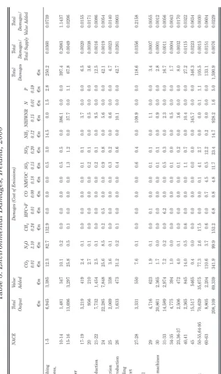
From Table 5 one can see that, not unexpectedly, mining and agriculture stand out as the least environmentally efficient sectors. Taking agriculture, multiplying all emissions with their damage cost estimates and adding the results, the total environmental damage done amounts to €0.3 billion while total output is €6.9 billion. That is, for every €1.00 of output produced (value added) in agriculture, the amount lost in environmental damage is €0.04

9_{This number is the ratio of the total water demand and the annual expenditure on public water}

[image:13.556.80.397.86.621.2]

T

able 5:

Environmental Damages, Ireland, 2000

NACE

T

otal

V

alue

Damages (Cost of Emissions)

T otal T otal T otal Output Added Damages Damages/ Damages/ CO 2 N2 OC H4 HFC+F CO NMVOC SO 2 NO X NH 3 NHIWNR N P T otal Supply V alue Added

Damage Cost Estimates

0.01 3.10 0.24 0.01 0.00 0.18 0.15 0.20 0.12 0.15 0.01 0.59 € m € m € m € m € m € m € m € m € m € m € m € m € m € m € m Agriculture, forestry , fishing 1-5 6,945 3,385 12.3 82.7 132.9 0.0 0.0 0.0 0.5 3.0 14.5 0.0 1.5 2.8 250.2 0.0360 0.0739

Coal, peat, petroleum, ores,

quarrying 10-14 1,481 347 10.1 0.2 0.0 0.0 0.0 0.0 0.5 0.5 0.0 386.1 0.0 0.0 397.4 0.2683 1.1437

Food, beverage, tobacco

15-16 13,696 3,297 25.8 0.5 0.1 0.0 0.0 0.0 1.3 1.2 0.0 37.7 0.0 1.1 67.8 0.0049 0.0206 T

extiles Clothing Leather & Footwear

17-19 3,219 419 2.4 0.1 0.0 0.0 0.0 0.0 0.1 0.1 0.0 3.7 0.0 0.0 6 .5 0.0020 0.0155 W

ood & wood products

20 956 210 2.7 0.1 0.0 0.0 0.0 0.0 0.2 0.1 0.0 0.5 0.0 0.0 3 .6 0.0038 0.0171

Pulp, paper & print production

21-22 7,732 1,454 2.5 0.1 0.0 0.0 0.0 0.0 0.2 0.1 0.0 9.5 0.0 0.0 12.5 0.0016 0.0086 Chemical production 24 22,285 7,848 25.6 8.5 0.2 0.5 0.0 0.0 0.9 0.8 0.0 5.6 0.0 0.0 42.1 0.0019 0.0054

Rubber & plastic production

25 2,069 338 3.6 0.1 0.0 0.0 0.0 0.0 0.3 0.2 0.0 0.6 0.0 0.0 4 .7 0.0023 0.0140

Non-metallic mineral production

26 1,633 473 31.2 0.2 0.1 0.0 0.0 0.0 0.4 0.6 0.0 10.1 0.0 0.0 42.7 0.0261 0.0903

Metal production excluding

machinery & transport equipment

27-28 3,331 550 7.6 0.1 0.0 0.0 0.0 0.0 0.6 0.4 0.0 109.9 0.0 0.0 118.6 0.0356 0.2158

Agriculture & industrial

machinery 29 4,716 623 1.9 0.1 0.0 0.1 0.0 0.0 0.1 0.1 0.0 1.1 0.0 0.0 3 .4 0.0007 0.0055

Office and data process machines

30 20,861 2,365 1.7 0.0 0.0 0.0 0.0 0.0 0.1 0.1 0.0 0.9 0.0 0.0 2 .8 0.0001 0.0012 Electrical goods 31-33 14,589 2,974 7.2 0.2 0.0 6.2 0.0 0.0 0.5 0.3 0.0 2.3 0.0 0.0 16.7 0.001 1 0.0056 T ransport equipment 34-35 4,775 394 1.0 0.0 0.0 0.0 0.0 0.0 0.1 0.0 0.0 0.5 0.0 0.0 1 .7 0.0004 0.0043 Other manufacturing 23,36-37 2,506 472 4.0 0.1 0.0 0.0 0.0 0.0 0.1 0.2 0.0 3.6 0.0 0.0 8 .0 0.0032 0.0170 Fuel, power , water 40,41 2,365 845 14.0 0.5 0.6 0.0 0.0 0.0 1.1 0.7 0.0 10.4 0.0 0.0 27.2 0.01 15 0.0322 Construction 45 15,517 5465 0.4 0.0 0.0 0.0 0.0 0.0 0.0 0.0 0.0 345.7 0.0 0.0 346.3 0.0223 0.0634

Services, excl. transport

50-55,64-95 70,629 35,675 77.3 2.6 17.5 0.0 0.0 0.1 4.1 2.7 0.0 0.0 0.1 1.1 105.5 0.0015 0.0030 T ransport 60-63 8,805 2,204 110.6 3.7 0.6 0.0 0.7 4.5 0.5 12.2 0.2 0.0 0.0 0.0 133.1 0.0151 0.0604 T otal 208,109 69,339 341.9 99.9 152.2 6.8 0.8 4.8 11.7 23.4 14.7 928.2 1.6 5.0 1,590.9 0.0076 0.0229 Notes: Climate: CO 2

= carbon dioxide; N

2

O = nitrous oxide; CH

4

= methane; HFC+F = hydrofluorocarbons and fluorinated gases; CO = carbon monoxide; NMVOC = non-metallic volatile organic compo

unds, excl.

methane; Acidification;

SO

2

= sulphur dioxide; NO

X

= nitrogen oxides (NO and NO

2

); NH

3

= ammonia; W

aste:

A

W

= agricultural waste; HIWNR = hazardous industrial waste, not recycled; HIWR = hazardous

industrial waste, recycled; NHIWNR = non-hazardous industrial waste, not recycled; NHIWR = non-hazardous industrial waste, recy

cled; Eutrophication: BOD = organic matter (biological oxygen demand): N =

nitrogen; P

=

phosphorus. Damage costs: CO

2

: global damage less than $50/tC (T

ol, 2005); N

2

O, CH

4

, HFC+F: CO

2

times global warming potential (296, 23); CO, NO

x

: average of Romilly (1999) and Spitley

et al

.

(2005); VOC: Spitzley

et al.

(2005); SO

2

: Romilly (1999); NH

3

, N, P: Pretty

et al.

(2000); NHIWNR: Forfás (2006); H

2

(€0.07). Methane emissions are the largest contribution (53 per cent), followed by nitrous oxide (33 per cent) and ammonia (6 per cent) emissions. Actually, mining is the least environmentally efficient sector, losing 27 cents for every euro of output produced, 97 per cent of which is due to waste.10_{Mining in fact} causes more environmental damage than the value it adds to the economy, causing €1.14 worth of damage for every €1.00 of value added. Metal production comes third (after agriculture), losing 4 cents in every euro, 93 per cent of which is due to waste.

For the economy as a whole, less than 1 cent is lost on every euro of output and 2 cent is lost on every euro of value added. Of this, 58 per cent is due to waste, and 37 per cent due to greenhouse gas emissions. The total environ-mental damage of production is about €1.6 billion; 25 per cent is due to the mining industry, 22 per cent due to construction, and 16 per cent due to agriculture. Mining and agriculture are also among the least environmentally efficient industries. Construction ranks 4th, but is ten times bigger than metal production when measured by value added to the economy.

Although the damage estimates are crude, they do allow us to identify the largest environmental problems (waste, climate change) and the dirtiest sectors (mining, agriculture and metal production if measured in terms of average efficiency; mining, agriculture and construction if measured in terms of total pollution). This helps to target environmental pollution.

V FORECASTS

5.1 Constant Emission Coefficients

Tables A3 and A4 show scenarios of possible changes in the Irish economy out to 2020. Table A3 corresponds to the High Growth scenario of Barrett et al.

(2005), whereas Table A4 is based on their Low Growth alternative.11_These results were derived from the HERMESmodel of the Irish economy. Note that

the HERMESmodel has six service sectors while the model here has only two;

and that HERMEShas three industrial sectors where this model has sixteen. The scenario in Table A3 assumes continued rapid economic growth, whereas Table A4 presents a slower growth path. In both models, growth is fastest in industry and transport. Agriculture is projected to grow only slowly,

10_{Again, there may be an aggregation problem. Mining waste is unlike waste from other sectors;}

the bulk of the waste is earth and stone.

11_{The high growth scenario is presented as “… one in which the US economy does not adjust and}

while construction grows first but then declines. These scenarios are used only for illustration.

Table 6 shows what would happen to emissions, waste, and water use if the economy were to grow as in Table A3. Table 7 shows the equivalent for the low growth alternative (see Table A4). In both tables it is assumed that there would be no policy, technological or behavioural changes with regard to the environment; that is, emission coefficients stay constant at their 2000 levels. This, of course, is an unrealistic assumption. See below for a limited sensitivity analysis.

Under both scenarios, all indicators go up, some more slowly than economic growth (e.g., agricultural waste, ammonia, nitrogen, methane) and some faster (e.g., HFCs, carbon monoxide, hazardous industrial waste). Nitrogen oxides are projected to rise at a rate marginally above that for economic growth in the high growth scenario, but at a rate less than economic growth in the low growth alternative. Again, this is strictly illustrative. Policy, technology, and behaviour will change between now and 2020.

5.2 Falling Emission Coefficients

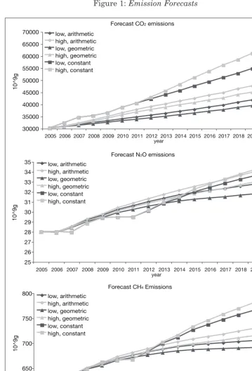
Emission coefficients are unlikely to stay constant. CSO (2006b) has emission data for selected greenhouse and acidifying gases, while sectoral economic activity can be downloaded from http://www.cso.ie. For these pollutants, emission coefficients have fallen consistently between 1994 and 2004. The year-on-year changes in emission intensities in the period 1994-2004 were used to construct both the arithmetic and geometric mean of changes in this period for each sector and pollutant.12_{These were then used to} extrapolate out to 2020 using the predicted growth rates of each sector shown in Tables A3 and A4. For comparison, a third trend is also shown wherein intensities were assumed not to change over the period, and thus emissions change only with changes in industry production (as above). The projected changes in emissions are shown in Figure 1 (see also Tables A5 to A10).

For carbon dioxide, there is a downward trend in emissions for most sectors, though the largest contributors (non-metallic mineral production, transport and services) will increase their emissions, ensuring an overall increase in carbon dioxide emissions. For nitrous oxide, there is a downward trend in emissions for most sectors, but the only contributor of note (agriculture) will increase its N₂O emissions. For methane, the largest contributors are agriculture and the services sector, which dwarf all other

12_{The geometric mean better reflects the exponential nature of growth but is, for short time}

[image:16.556.87.435.96.616.2]

T

able 6:

Emissions, W

aste, and Consumptive W

ater Use, Ireland, 2000-2020 – High Growth Scenario

Absolute

Index

2000

2005

2010

2015

2020

2000

2005

2010

2015

2020

CO

2

10^9 g

34,188.8

43,837.4

58,094.4

7,2014.9

88,180.3

100.0

128.2

169.9

210.6

257.9

N2

O

10^9 g

32.2

34.7

39.1

43.0

46.7

100.0

107.5

121.3

133.3

144.9

CH

4

10^9 g

634.2

675.6

744.2

803.0

858.0

100.0

106.5

1

17.3

126.6

135.3

HFC+F

10^9 g

678.2

881.1

1,238.3

1,548.5

1,855.6

100.0

129.9

182.6

228.3

273.6

CO

10^9 g

196.4

249.0

323.4

409.5

522.4

100.0

126.8

164.7

208.5

266.1

VOC

10^9 g

26.5

33.5

43.4

55.0

70.2

100.0

126.6

163.9

207.7

265.4

SO

2

10^9 g

78.2

101.1

134.8

165.2

199.1

100.0

129.4

172.5

21

1.4

254.8

NO

x

10^9 g

1

17.0

146.0

188.5

233.1

287.6

100.0

124.8

161.2

199.3

245.9

NH

3

10^9 g

122.4

126.5

135.6

143.0

148.9

100.0

103.3

1

10.8

1

16.8

121.6

A

W

10^9 g

56,516.2

58,190.8

62,161.7

65,245.5

67,546.0

100.0

103.0

1

10.0

1

15.4

1

19.5

HIWNR

10^9 g

120.9

157.1

220.0

273.2

325.2

100.0

129.9

182.0

225.9

269.0

HIWR

10^9 g

132.4

172.1

240.2

296.1

350.0

100.0

130.0

181.4

223.6

264.3

NHIWNR

10^9 g

6,187.8

8,048.3

10,781.5

12,013.3

12,654.2

100.0

130.1

174.2

194.1

204.5

NHIWR

10^9 g

7,369.1

9,593.2

12,324.0

12,188.4

10,772.4

100.0

130.2

167.2

165.4

146.2

BOD

10^9 g

34.8

42.5

55.7

67.2

78.6

100.0

122.3

160.2

193.2

226.0

N

10^9 g

160.3

168.3

183.6

196.2

207.0

100.0

105.0

1

14.5

122.4

129.1

P

10^9 g

8.4

9.7

1

1.6

13.4

15.1

100.0

1

15.0

138.5

159.3

180.0

H2

O

10^6 l

232,926

259,646

309,565

351,888

391,665

100.0

1

1

1.5

132.9

151.1

168.1

GDP

at

factor cost

10^6

€

208,109 269,253

359,027

432,742

506,527

100.0

129.4

172.5

207.9

243.4

Notes:

Climate: CO

2

= carbon dioxide; N

2

O = nitrous oxide; CH

4

= methane; HFC+F = hydrofluorocarbons and fluorinated gases; CO = carbon monoxide; NMVOC

= non-metallic volatile organic compounds, excl. methane;

Acidification; SO

2

= sulphur dioxide; NO

x

= nitrogen oxides (NO and NO

2

); NH

3

= ammonia; W

aste:

A

W

= agricultural waste; HIWNR = hazardous industrial waste, not recycled; HIWR = hazardous industrial waste, recycled; NHIWNR = n

on-hazardous industrial waste,

not recycled; NHIWR = non-hazardous industrial waste, recycled; Eutrophication: BOD = organic matter (biological oxygen demand)

: N = nitrogen; P

=

[image:17.556.81.394.89.616.2]

T

able 7:

Emissions, W

aste, and Consumptive W

ater Use, Ireland, 2000-2020 – Low Growth Scenario

Absolute

Index

2000

2005

2010

2015

2020

2000

2005

2010

2015

2020

CO

2

10^9 g

34,188.8

43,837.4

53,949.7

64,224.7

77,053.5

100.0

128.2

157.8

187.9

225.4

N2

O

10^9 g

32.2

34.7

38.3

41.3

43.9

100.0

107.5

1

18.7

128.0

136.1

CH

4

10^9 g

634.2

675.6

737.6

784.2

817.6

100.0

106.5

1

16.3

123.6

128.9

HFC+F

10^9 g

678.2

881.1

1,104.0

1

,336.9

1,621.2

100.0

129.9

162.8

197.1

239.0

CO

10^9 g

196.4

249.0

304.6

365.9

444.5

100.0

126.8

155.1

186.3

226.4

VOC

10^9 g

26.5

33.5

40.9

49.1

59.6

100.0

126.6

154.6

185.7

225.4

SO

2

10^9 g

78.2

101.1

125.1

148.0

176.9

100.0

129.4

160.0

189.4

226.3

NO

x

10^9 g

1

17.0

146.0

177.1

209.5

249.9

100.0

124.8

151.4

179.1

213.7

NH

3

10^9 g

122.4

126.5

135.4

141.5

143.9

100.0

103.3

1

10.6

1

15.6

1

17.6

A

W

10^9 g

56,516.2

58,190.8

62,137.9

64,725.3

65,539.4

100.0

103.0

109.9

1

14.5

1

16.0

HIWNR

10^9 g

120.9

157.1

196.9

237.2

286.0

100.0

129.9

162.9

196.2

236.5

HIWR

10^9 g

132.4

172.1

215.8

258.5

309.7

100.0

130.0

162.9

195.2

233.9

NHIWNR

10^9 g

6

,187.8

8

,048.3

10,1

17.4

1

1

,297.9

12,385.8

100.0

130.1

163.5

182.6

200.2

NHIWR

10^9 g

7

,369.1

9

,593.2

12,090.9

12,549.3

12,327.6

100.0

130.2

164.1

170.3

167.3

BOD

10^9 g

34.8

42.5

51.2

59.9

70.0

100.0

122.3

147.3

172.2

201.3

N

10^9 g

160.3

168.3

182.2

192.3

198.4

100.0

105.0

1

13.7

120.0

123.8

P

10^9 g

8

.4

9.7

1

1.1

12.4

13.8

100.0

1

15.0

132.4

148.2

164.9

H2

O

10^6 l

232,926.0

259,646.2

294,942.3

327,484.2

360,596.6

100.0

1

1

1.5

126.6

140.6

154.8

GDP

at

factor cost

10^6

€

208,109 269,253

332,754

389,475

455,692

100.0

129.4

159.9

187.1

2,19.0

Notes:

Climate: CO

2

= carbon dioxide; N

2

O = nitrous oxide; CH

4

= methane; HFC+F = hydrofluorocarbons and fluorinated gases; CO = carbon

monoxide; NMVOC = non-metallic volatile organic compounds, excl. methane;

Acidification; SO

2

= sulphur dioxide; NOx = nitrogen oxides (NO

and NO

2

); NH

3

= ammonia; W

aste:

A

W

= agricultural waste; HIWNR = hazardous industrial waste, not recycled; HIWR = hazardous industrial

waste, recycled; NHIWNR = non-hazardous industrial waste, not recycled; NHIWR = non-hazardous industrial waste, recycled; Eutro

phication:

BOD = organic matter (biological oxygen demand): N = nitrogen; P

=

Forecast CO2 emissions

30000 35000 40000 45000 50000 55000 60000 65000 70000

2005 2006 2007 2008 2009 2010 2011 2012 2013 2014 2015 2016 2017 2018 2019 2020 year

10^9g

low, arithmetic high, arithmetic low, geometric high, geometric low, constant high, constant

Forecast N2O emissions

25 26 27 28 29 30 31 32 33 34 35

2005 2006 2007 2008 2009 2010 2011 2012 2013 2014 2015 2016 2017 2018 2019 2020 year

10^9g

low, arithmetic high, arithmetic low, geometric high, geometric low, constant high, constant

Forecast CH4 Emissions

600 650 700 750 800

2005 2006 2007 2008 2009 2010 2011 2012 2013 2014 2015 2016 2017 2018 2019 2020 year

10^9g

[image:18.556.77.437.96.626.2]

low, arithmetic high, arithmetic low, geometric high, geometric low, constant high, constant

Forecast SO2 emissions

15 25 35 45 55 65 75 85

2005 2006 2007 2008 2009 2010 2011 2012 2013 2014 2015 2016 2017 2018 2019 2020 year

10^9g

low, arithmetic high, arithmetic low, geometric high, geometric low, constant high, constant

Forecast NOX emissions

70 90 110 130 150 170

2005 2006 2007 2008 2009 2010 2011 2012 2013 2014 2015 2016 2017 2018 2019 2020 year

10^9g

low, arithmetic high, arithmetic low, geometric high, geometric low, constant high, constant

Forecast NH3 emissions

110 115 120 125 130 135 140 145 150

2005 2006 2007 2008 2009 2010 2011 2012 2013 2014 2015 2016 2017 2018 2019 2020 year

10^9g

[image:19.556.70.427.97.617.2]

low, arithmetic high, arithmetic low, geometric high, geometric low, constant high, constant

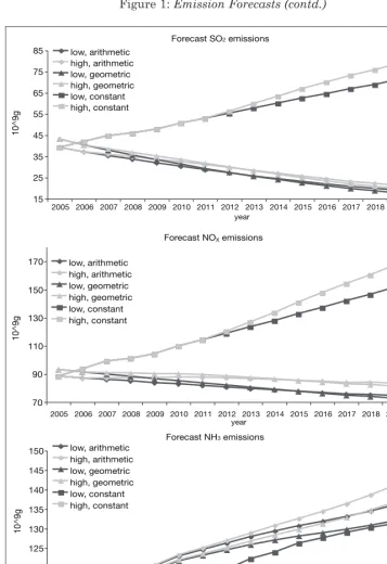
sectors. Agricultural emissions are set to continue rising out to 2020,13_with emissions in services set to remain largely constant. The overall trend is for increased methane emissions, however. For sulphur dioxide, all sectors show a reduction in emissions out to 2020. The largest of these contributors – the services sector (excluding transport) – will reduce its emissions by around 50 per cent compared to 2004 levels. For oxides of nitrogen, there is a downward trend in emissions for the largest contributors (agriculture, transport and services) that will lead to an overall decline in emissions of NO_x. However, there will be large percentage increases for some industries that currently emit relatively low levels of NO_x(mining, non-metallic mineral production and textiles and clothing). For ammonia, emissions from agriculture are set to rise slowly out to 2020, though this is from a relatively high base. Conversely, the transport sector will see ammonia emissions rise by between 550 per cent (assuming a low growth rate, and calculated using a geometric mean) and 700 per cent (assuming a high growth rate, and calculated using an arithmetic mean), but from a much lower level compared to agriculture.

For all of the pollutants discussed here, the high-growth scenario would result in higher levels of emissions than in the low growth alternative, and predicted emissions are higher when an arithmetic mean is used to calculate future trends. This can be seen in Figure 1.

It is also clear that the projections based on constant emission coefficients overestimate future emissions. This is particularly striking for emissions of sulphur and oxides of nitrogen, where technological progress changes the sign of the change, but it can also be seen for the other pollutants.

VI CONCLUSIONS

An environmental input-output model, ISus 0.0, was constructed for Ireland for the year 2000. The model results confirm that certain sectors pollute more than others – even when normalised by the sectoral value added. Mining, agriculture, metal production and construction stand out as the dirtiest industries. Most sectors add more value than they do environmental damage. However, the dirtiest industry, mining, does 127 cents worth of damage for every euro of value added. For the Irish economy as a whole, only 1 cent is lost in damage for every euro earned. Waste and greenhouse gas emissions are the largest environmental problems. The environmental impact of consumption is very different from the impact of production because of the

13_{The HERMESmodel predicts that agricultural emissions will continue to rise out to 2020.}

intermediary deliverables. We find differences up to a factor of 1.5 million, in case production is ‘clean’ but intermediates are ‘dirty’. Even without technological progress, behavioural changes, and policy interventions, most environmental problems will increase more slowly than the rate of economic growth, with the exception of fluorinated gases, carbon monoxide, and hazardous industrial waste. For the subset of pollutants for which data are available, emission intensity falls. For sulphur, emission intensities fall sufficiently fast to more than offset economic growth. When a forecast is constructed of emissions out to 2020, certain trends become apparent. Emissions of greenhouse gases (CO₂, N₂O and CH₄) will increase, while emissions of acid rain gases (SO₂, NO_xand NH₃) will decrease.

These results should be treated with caution. The results for waste and eutrophication are particularly weak. Partly, this is a matter of data – the analysis here is restricted to data in the public domain. Furthermore, waste and eutrophication are not national, but regional phenomena. The same holds true for water. A regional analysis would require either regionalising the national results, or using a regional input-output model for crucial sectors (e.g., agriculture). Either route would be constrained by data availability. Further improvement of the sectoral disaggregation would be needed too – as demonstrated by the methane emissions attributed to the wood products sector. A finer categorisation of ‘waste’ would be welcome too. Emission coefficients are here assumed to be static, but in fact respond to structural changes within the economic sectors, technological changes, prices, and environmental policies. Finally, input-output analysis focuses on the production side of the domestic economy. Household pollution and resource use is not included. This particularly affects carbon dioxide, waste and water. Similarly, the environmental impacts of the production of imported goods are excluded.

It is evident that much remains to be done in developing a thorough model of environment-economy relationships in Ireland. The results presented here may prove to be a useful first step. Later versions of the ISus model will address the weaknesses of the current model and paper.

REFERENCES

AERTEBJERG, GUNNI and JACOB CARSTENSEN, 2003. Chlorophyll-a in

Transitional, Coastal and Marine Waters, Copenhagen: European Environment Agency.

BARRETT, ALAN and JOHN LAWLOR, 1995. The Economics of Solid Waste

BARRETT, ALAN, ADELE BERGIN, DAVID DUFFY, SHANE GARRETT, JOHN FITZ

GERALD, IDE KEARNEY and YVONNE MCCARTHY, 2005. Medium-Term

Review 2005-2012, Dublin: The Economic and Social Research Institute.

BEHAN, JESMINA and KIERAN MCQUINN, 2002. Projecting Net Greenhouse Gas

Emissions from Irish Agriculture and Forestry [online], Available from http://www.tnet.teagasc.ie/fapri/downloads/esri.pdf.

BERGIN, ADELE, JOE CULLEN, DAVID DUFFY, JOHN FITZ GERALD, IDE

KEARNEY and DANIEL MCCOY, 2003. Medium-Term Review: 2003-2010,

Dublin: The Economic and Social Research Institute.

CAMP DRESSER and MCKEE, 2004. Economic Analysis of Water Use in Ireland,

Dublin: Department of the Environment, Heritage and Local Government. CONNIFFE, DENIS, JOHN FITZ GERALD, SUE SCOTT, and FERGAL SHORTALL,

1997. The Costs to Ireland of Greenhouse Gas Abatement, Policy Research Series

No 32, Dublin: The Economic and Social Research Institute.

CENTRAL STATISTICS OFFICE, 2006a. 2000 Supply and Use and Input-Output

Tables, Cork: Central Statistics Office.

CENTRAL STATISTICS OFFICE, 2006b. Environmental Accounts for Ireland

1997-2004, Cork: Central Statistics Office.

DELLINK, ROB, MARTIJN BENNIS and HARMEN VERBRUGGEN, 1999.

“Sustainable Economic Structures” Ecological Economics, Vol 29, pp 141-154.

DEPARTMENT OF PUBLIC ENTERPRISE, 2000. Environmental Impacts of Irish

Transport Growth and of Related Sustainable Policies, Report prepared by Oscar Faber Transportation in association with ECOTEC Research & Consulting Ltd., Goodbody Economic Consultants Limited and The Economic and Social Research Institute [online], Available from: http://www.transport.ie/upload/general/2637.pdf.

DUCHIN, FAYE and GLENN-MARIE LANGE, 1994. The Future of the Environment:

ecological economics and technical change, Oxford: Oxford University Press.

EUROPEAN ENVIRONMENT AGENCY, 2005. May 2005 Assessment [online],

available from http://themes.eea.europa.eu/IMS/IMS/ISpecs/ISpecification2004 1007131526/IAssessment1116513959574/view_content.

ENVIRONMENT PROTECTION AGENCY, 2005a. Irish Submission to the United

Nations Framework Convention on Climate Change, Johnstown Castle: Environ-mental Protection Agency.

ENVIRONMENT PROTECTION AGENCY, 2005b. National Waste Report 2004,

Johnstown Castle: Environmental Protection Agency.

FITZ GERALD, JOHN, 2004. “An Expensive Way to Combat Global Warming: Reform

Needed in EU Emissions Trading Regime” Quarterly Economic Commentary

(Spring 2004), Dublin: The Economic and Social Research Institute.

GREN, ING-MARIE, THOMAS SOEDERQVIST, and FREDRIC WULFF, 1997.

“Nutrient Reductions to the Baltic Sea: Ecology, Costs and Benefits”, Journal of

Environmental Management, Vol 51, pp. 123-143.

HENDRICKSON, CHRIS T., LESTER B. LAVE, H. SCOTT MATTHEWS, ARPAD

HORVATH, SATISH JOSHI, FRANCIS C. MCMICHAEL, HEATHER MACLEAN,

GYORGYI CICAS, DEANNA MATTHEWS and JOULE BERGERSON 2006.

Environmental Life-Cycle Assessment of Goods and Services: An Input-Output Approach, Washington, D.C.: Resources for the Future.

LEONTIEF, WASSILY, 1970. “Environmental Repercussions and the Economic

Structure: An Input-Output Approach”, Review of Economics and Statistics,Vol 52,

No 3, pp. 262-271.

GERT VAN DER BIJL, 2000. “An Assessment of Total External Costs of UK

Agriculture”, Agricultural Systems,Vol 65, pp. 113-136.

PRETTY, JULES, CHRISTOPHER F. MASON, DAVID B. NEDWELL, RACHEL E. HINE, SIMON LEAF and RACHAEL DILS, 2003. “Environmental Costs of

Freshwater Eutrophication in England and Wales”, Environmental Science and

Technology,Vol 37, No 2, pp. 201-208.

RAMASWAMY, VENKATACHALA, OLIVIER BOUCHER, JOANNA D. HAIGH, DIDIER HAUGLUSTAINE, JAMES HAYWOOD, GUNNAR MYHRE, TERUYUKI NAKAJIMA, GUANGYU SHI and SUSAN SOLOMON, 2001. “Radiative Forcing

of Climate Change” in John T. Houghton and Yihui Ding (eds.), Climate Change

2001: The Scientific Basis – Contribution of Working Group I to the Third Assessment of the Intergovernmental Panel on Climate Change, Cambridge: Cambridge University Press.

RAVETZ, JOE, DARRYN MCEVOY, SARAH LINDLEY and JOHN HANDLEY, 2003.

Linking Up: Linking Environmental-Economic Modelling into Sustainable Planning in Wales and the Regions, Environment Agency R&D Technical Report E2-058/TR [online], Available from http://www.sed.manchester.ac.uk/research/ cure/ downloads/reward_main.pdf.

ROMILLY, PETER, 1999. “Substitution of Bus for Car Travel in Urban Britain: An Economic Evaluation of Bus and Car Exhaust Emission and Other Costs”,

Transportation Research Part D, Vol. 4, pp. 109-125.

SCOTT, SUE,1999. Pilot Environmental Accounts, Cork: Central Statistics Office.

SCOTT, SUE, 2004. Research Needs of Sustainable Development, ESRI Working Paper

No 162, Dublin: The Economic and Research Institute.

SCOTT, SUE, JOHN CURTIS, JOHN EAKINS, JOHN FITZ GERALD and

JONATHAN HORE, 2001. Time Series and Eco-Taxes: Energy, Water, Waste,

Report for EUROSTAT (B1 section: National Accounts methodology, statistics for own resources), Ref KITZ99/274.

SPITZLEY, DAVID V., DARBY E.GRANDE, GREGORY A. KEOLEIAN AND HYUNG CHUL KIM, 2005. “Life Cycle Optimization of Ownership Costs and Emission

Reduction in US Vehicle Retirement Decisions”, Transportation Research Part D,

Vol. 10, pp. 161-175.

TONER, PAUL, JIM BOWMAN, KEVIN CLABBY, JOHN LUCEY, MARTIN

MCGARRIGLE, COLMAN CONCANNON, CONOR CLENAGHAN, PETER

CUNNINGHAM, JOHN DELANEY, SHANE O’BOYLE, MICHAEL

MACCÁRTHAIGH, MATTHEW CRAIG and R. QUINN, 2005. Water Quality in

Ireland 2001-2003, Wexford: Environmental Protection Agency.

TOL, RICHARD S.J., 2005. “The Marginal Damage Costs of Carbon Dioxide Emissions:

An Assessment of the Uncertainties”, Energy Policy, Vol 33, No. 16, pp. 2064-2074.

TRENT, ZOE, 2003. National River Classification Schemes, European Environment

Agency, Copenhagen.

TURNER, R. KERRY, STAVROS GEORGIOU, ING-MARIE GREN, FREDRIC WULFF, SCOTT BARRETT, TORE SOEDERQVIST, IAN J. BATEMAN, CARL FOLKE, SINDRE LANGAAS, TOMASZ ZYLICZ, KARL-GOERAN MALER and AGNIESZKA MARKOWSKA, 1999. “Managing Nutrient Fluxes and Pollution in

the Baltic: An Interdisciplinary Simulation Study’” Ecological Economics, Vol. 30,

pp. 333-352.

VAN DEN BERGH, JEROEN C.J.M. and MARJAN W. HOFKES, 1999. “Economic Models of Sustainable Development” in Jeroen C. J. M. Van den Bergh (ed.),