Efficient Learning of Random Forest Classifier using Disjoint Partitioning Approach

Efficient Learning of Random Forest

Classifier using Disjoint Partitioning Approach

Vrushali Y Kulkarni Pradeep K Sinha

Abstract - Random Forest is an Ensemble Supervised Machine Learning technique. Research work in the area of Random Forest aims at either improving accuracy or improving performance. In this paper we are presenting our research towards improvement in learning time of Random Forest by proposing a new approach called Disjoint Partitioning. In this approach, we are using disjoint partitions of training dataset to train individual base decision trees. This helps in creating diversity in base decision trees. Also different subsets of attributes are used at each node of decision tree to increase diversity. This approach generates Random Forest classifier which is trained efficiently and gives classification accuracy comparable to the original Random Forest approach.

Index Terms - Random Forest, Classification, Decision Tree, Disjoint Partitioning, Learning

I. INTRODUCTION

Random Forest (RF) is an ensemble supervised machine learning algorithm. Machine learning techniques are applied in the domain of Data Mining [8]. Random Forest [Breiman 2001] uses decision tree as base classifier. Random Forest generates multiple decision trees; the randomization is present in two ways: first random sampling of data for bootstrap samples as it is done in bagging and second random selection of input attributes for generating individual base decision trees. Strength of individual decision tree and correlation among base trees are key issues which decide generalization error of Random Forest classifier [3]. Based on accuracy measure, Random Forest classifier is at par with existing ensemble techniques like bagging [1] and boosting [6]. As per Brieman, Random Forest runs efficiently on large databases, it can handle thousands of input variables without variable deletion, it gives estimates of important variables, it generates an internal unbiased estimate of generalization error as forest growing progresses, it has effective method for estimating missing data and maintains accuracy when a large proportion of data are missing, and it has methods for balancing class error in class population unbalanced data sets [3]. The inherent parallel nature of Random Forest has led to its parallel

Vrushali Y Kulkarni is an Associate Professor, of MIT, Pune, India and a Research Scholar, College of Engineering, Pune, India

(Email: [email protected], [email protected]) Pradeep K Sinha is a Senior Director, HPC, CDAC, Pune, India

implementations using multithreading, multi-core, and parallel architectures. Random Forest is used in many recent classification and prediction applications [13] due to above mentioned features.

It has been proved theoretically and empirically that the ensemble always gives better accuracy than an individual classifier [2]. The fundamental of ensemble design is creating diversity among the base classifiers [5]. Random Forest is based on the principle of bagging. Instable base learners are good choice for bagging ensembles [1]. Decision Tree is instable in nature and hence works well as base classifier with Random Forest. As in bagging, bootstrap samples are generated for induction of each decision tree. Another source of randomization is introduced through attribute selection. Research work in the area of Random Forest aims at either improving accuracy or improving performance i.e. reducing time required for learning and classification, or both. Some work aims at experimentation with Random Forest using online continuous stream data which is very much essential today due to data streams getting generated as a result of various applications. Random Forest being ensemble technique, experiments are done with its base classifier, e.g. Fuzzy Decision Tree as base classifier of Random Forest. We have done in depth and systematic survey of current ongoing research on Random Forest and also developed “Taxonomy of Random Forest Classifier” [14].

The research work on improving accuracy is by Robnik-Sikonja [7]. They have generated base trees of Random Forest using different split measures and also applied weighted voting. In [9] it is demonstrated that accuracy of random forest is improved in some domains by replacing majority voting with Dynamic Integration, which is based on local prediction performances of base decision trees. In [10], Random Forest themselves are used as base classifiers for making ensemble called Meta Random Forest, and the accuracy of this model is tested and compared with the existing Random Forest algorithm.

tree. This ensures diversity among individual trees. Another measure taken to increase diversity is use of less correlated attributes. For this, at each node, we are selecting (2/3)*m features out of total m features and then selecting √m features randomly to decide best split at each node (which is the process for induction of Random Forest that is to be explained in the next section). Here as each individual tree is trained with less number of samples, the learning of each tree and hence learning of forest is more efficient.

This paper is organized in the following way: section II explains in brief the working of Random Forest classifier. Section III describes Disjoint Partitioning approach for Random Forest. Section IV presents Results and Discussions. Section V gives Concluding Remarks.

II. RANDOM FOREST

Definition: A Random Forest is a classifier consisting of a collection of tree-structured classifiers {h(x, Θk) k=1, 2, ….}, where the {Θk } are independent identically distributed random vectors and each tree casts a unit vote for the most popular class at input x [3].

Random Forest generates an ensemble of decision trees. To generate each single tree in Random Forest, Breiman followed following steps: If the number of records in the training set is N, then N records are sampled at random but with replacement, from the original data; this is bootstrap sample. This sample will be the training set for growing the tree. If there are M input variables, a number m << M is selected such that at each node, m variables are selected at random out of M and the best split on these m attributes is used to split the node. The value of m is held constant during forest growing. Each tree is grown to the largest extent possible. There is no pruning.

In this way, multiple trees are induced in the forest; the number of trees is pre-decided by the parameter Ntree. The number of variables (m) selected at each node is also referred to as mtry or k in the literature. The depth of the tree can be controlled by a parameter nodesize (i.e. number of instances in the leaf node) which is usually set to one.

Once the forest is trained or built as explained above, to classify a new instance, it is run across all the trees grown in the forest. Each tree gives classification for the new instance which is recorded as a vote. The votes from all trees are combined and the class for which maximum votes are counted (majority voting) is declared as classification of the new instance.

This process is referred to as Forest RI in the literature [3]. Here onwards, Random Forest means the forest of decision trees generated using Forest RI process.

In the forest building process, when bootstrap sample set is drawn by sampling with replacement for each tree, about 1/3rd of original instances are left out. This set of instances is called OOB (Out-of-bag) data. Each tree has its own OOB data set which is used for error estimation of individual tree in the forest, called as OOB error estimation.

The Generalization error of Random Forest is given as,

PE * _{= P}

x,y (mg(X,Y)) < 0 The margin function is given as,

mg (X,Y) = avk I(hk (X) = Y) – max j≠Y avk I(hk (X) = j)

The margin function measures the extent to which the average number of votes at (X, Y) for the right class exceeds the average vote for any other class. Strength of Random Forest is given in terms of the expected value of margin function as,

S = E X, Y (mg (X, Y))

If ρ is mean value of correlation between base trees, an upper bound for generalization error is given by,

PE* ≤ρ (1 – s2_{) / s}2

Hence, to yield better accuracy in Random Forest, the base decision trees are to be diverse and accurate.

III.

D

P

A

The process of Disjoint Partitioning is as given below:

Experimental Protocol – Disjoint Partitioning

Input:

N : Size of training dataset D A : Attribute space (A1, A2, …, Am)

m : Total number of attributes of training data set n : Total number of trees to be generated in Random Forest

t : Size of each partition nodesize: size of leaf node

// tree creation stops when nodesize records are remaining in the node

Output:

A Random Forest R

Method t = N/n

q = 2/3*m or 1/3*m for i = 1 to n do

Randomly sample t instances from D without replacement to generate partition Pi

Discard these t instances from D end for

for i = 1 to n do

1. generate base decision tree Ti using following steps 2. for each node in Ti

3. select subset of attributes Ainew = (A1, A2, …, Aq) randomly without replacement from attribute space A 1. k = √m

2. Select k attributes from Ainew randomly without replacement

3. decide best split on these k attributes 4. end for

5. end for //loop ends at stopping criterion i.e. nodesize

end Experimental Protocol

IV. METHODS AND RESULTS

Original Random Forest and Disjoint Partitioning approach are compared on the basis of time for learning, and accuracy. The datasets selected are all from UCI machine learning repository. We have tested this approach on many datasets and found out that the approach works well on datasets which are highly imbalanced in nature (especially datasets from medical diagnosis field). To support our observation, we have generated two synthetic datasets of imbalanced nature using Agrawal generator from weka tool. The details of datasets for which results are presented in this paper are given in Table I. For every dataset, we have varied number of trees in Random Forest from 2 to 10. This is done because for datasets of moderate size, generating more number of disjoint partitions from dataset will affect learning negatively. Also learning of Random Forest will be efficient if it contains less number of trees. Along with this, time taken to build Random Forest is also recorded in each case. To ensure that accuracy achieved

with Disjoint partitioning approach is comparable with Random Forest, the original Random Forest is run by varying number of trees from 2 to 100. If maximum accuracy is not obtained within first 2 to 10 trees, then the maximum accuracy value between 11 to 100 trees, number of trees for getting maximum accuracy, and time taken is recorded. Readings are taken for Disjoint Partitioning with attribute subset as (1/3*m) where m is total number of attributes – this is called as DP (1/3) and Disjoint Partitioning with attribute subset as (2/3*m) – called as DP (2/3).

All the experimentation is done using Weka tool with 10 – fold cross-validation. Readings for time taken to learn the forest are in seconds. With weka tool, we were able to record time up to millisecond level. Hence the time values below milliseconds are recorded as 0.

Table II gives readings for Maximum % Accuracy and Learning Time for the datasets presented in Table I. It also contains the number of trees for which the maximum

accuracy is achieved. The experimental readings are proving that with Disjoint Partitioning approach, Random Forest learns in less time and at least with the same or increased accuracy as that of the original Random Forest.

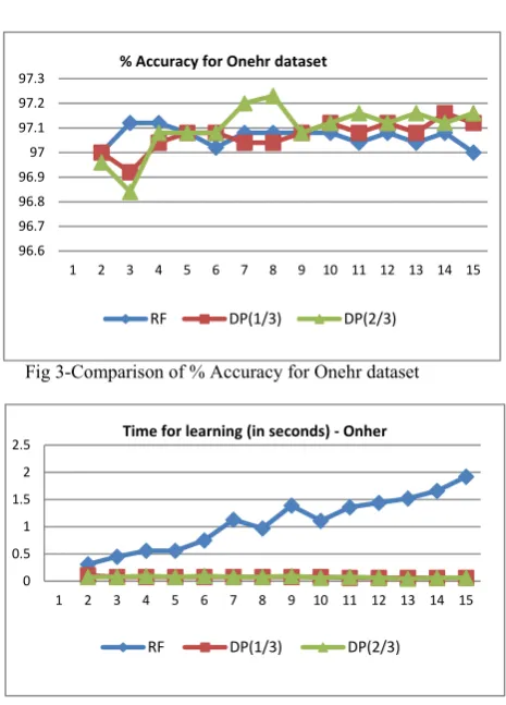
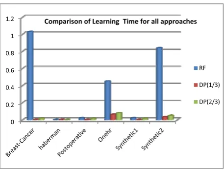
We have also presented here graphs for % Accuracy and Learning time values for RF, DP (1/3) and DP (2/3) for Breast cancer dataset (fig 1 and fig 2) and Onehr dataset (fig 3 and fig 4). The comparative analysis of % Accuracy and Learning time for all the three approaches for all datasets are presented in fig 5 and fig 6 respectively.

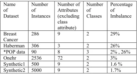
Table I- Details of datasets for which results are presented

Name of Dataset

Number of Instances

Number of Attributes (excluding class attribute)

Number of Classes

Percentage of Imbalance

Breast

Cancer 286 9 2 29%

Haberman 306 3 2 26%

*POP data 90 8 3 2% , 26%

Onehr 2536 72 2 3%

Synthetic1 500 9 2 1.6 %

Synthetic2 5000 9 2 1.7%

V. CONCLUSION

Table II- Learning Time and Number of trees to achieve Maximum % Accuracy

Dataset % Accuracy Number of Trees Learning Time (in seconds) RF DP(1/3) DP(2/3) RF DP(1/3) DP(2/3) RF DP(1/3) DP(2/3) Breast Cancer 70.97 72.02 69.23 61 2 12 1.03 0 0.016

Haberman 66.99 71.24 71.24 2 3 3 0 0 0

POP data 66.33 67.77 68.88 2 4 11 0.02 0 0.015

Onehr 97.14 97.23 97.2 4 17 7 0.56 0.062 0.078

Synthetic1 98.4 98.4 98.8 2 2 2 0.02 0 0.015

Synthetic2 98.7 98.34 98.48 30 5 5 0.84 0.031 0.032

In table, 0 indicates time recorded is less than milli-seconds

DP(1/3) – Disjoint Partitioning approach with (1/3*m) attribute subset DP(2/3) – Disjoint Partitioning approach with (2/3*m) attribute subset

Fig 1-Comparison of % Accuracy for Breast Cancer dataset

Fig. 2-Comparison of learning time for Breast Cancer dataset

Fig 3-Comparison of % Accuracy for Onehr dataset

Fig 4-Comparison of learning time for Onehr dataset 62

64 66 68 70 72 74

1 2 3 4 5 6 7 8 9 10

% Accuracy for Breast Cancer dataset

RF DP(1/3) DP(2/3)

0 0.01 0.02 0.03 0.04

2 3 4 5 6 7 8 9 10

Time for learning (in seconds) ‐Breast cancer

RF DP(1/3) DP(2/3)

0 0.5 1 1.5 2 2.5

1 2 3 4 5 6 7 8 9 10 11 12 13 14 15

Time for learning (in seconds) ‐Onher

RF DP(1/3) DP(2/3)

96.6 96.7 96.8 96.9 97 97.1 97.2 97.3

1 2 3 4 5 6 7 8 9 10 11 12 13 14 15

% Accuracy for Onehr dataset

Fig 5 – Comparison of Maximum % Accuracy for all approaches

Fig 6-Comparision of Learning Time for all approaches

REFERENCES

[1] Leo Breiman, Bagging Predictors, Technical report No 421, September 1994

[2] David Opitz, Richard Maclin, “Popular Ensemble Methods: An Empirical Study”, Journal of Artificial Intelligence 11, 169-198, 1999

[3] Leo Brieman, “Random Forests”, Machine Learning, 45, 5-32, (2001)

[4] Latinne P, Debeir O, Decastecker C, Limiting the number of trees in Random Forest, MCS, UK (2001)

[5] L Kuncheva, C Whitaker, Measures of Diversity in Classifier Ensembles and their relationship with the Ensemble Accuracy, Machine Learning, 51, 181-207, (2003)

[6] Robert E Schapire, The Boosting Approach to Machine Learning an Overview, Nonlinear Estimation and Classification, Springer, 2003 [7] Marko Robnik, Sikonja, “Improving Random Forests”, J F

Boulicaut et al (eds): Machine Learning, ECML 2004 Proceedings, Springer, Berlin, 2004

[8] Jiawei Han and Micheline Kamber, “Data Mining: Concepts and Techniques” (2nd _{Edition), Morgan Kaufmann Publisher, (2006)}

[9] Tsymbal A, Pechenizkiy M, Cunningham P, Dynamic Integration with Random Forest, ECML, LNAI, 801-808, Springer-Verlag (2006)

[10] Boinee P, Angelis A, Foresti G, Meta Random Forest, International Journal of Computational Intelligence 2, (2006)

[11] Bernard S, Heutte L, Adam S, On the Selection of Decision Trees in Random Forest, Proceedings of International Joint Cobference on Neural Networks, Atlanta, Georgia, USA, June 14-19,302-307, (2009)

[12] Bernard S, Heutte L, Adam S, Towards a Better Understanding of Random Forests Through the Study of Strength and Correlation, ICIC Proceedings of the Intelligent Computing 5th International Conference on Emerging Intelligent Computing Technology and Applications, (2009)

[13] Verikas A, Gelzinis A, Bacauskiene M, Mining data with random forests: A survey and results of new tests, Pattern Recognition 44 , 330 - 349, (2011)

[14] Vrushali Y Kulkarni, Pradeep K Sinha, Random Forest Classifiers: A Survey and Future Research directions, Int Journal of Advanced Computing, Vol 36 Issue 1, pages 1144-1153, (2013)

[15] Bernard S, Heutte L, Adam S, Dynamic Random forests, Pattern Recognition Letters, 33 (2012), 1580-1586

0 20 40 60 80 100

Maximum %Accyracy for all approaches

RF DP(1/3) DP(2/3)

0 0.2 0.4 0.6 0.8 1 1.2

RF DP(1/3) DP(2/3)