The Thirty-Third AAAI Conference on Artificial Intelligence (AAAI-19)
A Two-Individual Based Evolutionary
Algorithm for the Flexible Job Shop Scheduling Problem
Junwen Ding,
1Zhipeng L ¨u,
1,∗Chu-Min Li,
2Liji Shen,
3Liping Xu,
1Fred Glover
4 1School of Computer Science, Huazhong University of Science and Technology, Wuhan, China2MIS, University of Picardie Jules Verne, Amiens, France
3Operations Management, WHU-Otto Beisheim School of Management, Vallendar, Germany 4College of Engineering & Applied Science, University of Colorado, Colorado, USA
{dingjunwen,zhipeng.lv,xlphust}@hust.edu.cn, [email protected], [email protected], [email protected]
Abstract
Population-based evolutionary algorithms usually manage a large number of individuals to maintain the diversity of the search, which is complex and time-consuming. In this pa-per, we propose an evolutionary algorithm using only two individuals, called master-apprentice evolutionary algorithm (MAE), for solving the flexible job shop scheduling problem (FJSP). To ensure the diversity and the quality of the evo-lution, MAE integrates a tabu search procedure, a recombi-nation operator based on path relinking using a novel dis-tance definition, and an effective individual updating strat-egy, taking into account the multiple complex constraints of FJSP. Experiments on 313 widely-used public instances show that MAE improves the previous best known results for 47 instances and matches the best known results on all ex-cept 3 of the remaining instances while consuming the same computational time as current state-of-the-art metaheuristics. MAE additionally establishes solution quality records for 10 hard instances whose previous best values were established by a well-known industrial solver and a state-of-the-art exact method.
Introduction
The job shop scheduling problem (JSP) is a strongly NP-hard problem (Garey, Johnson, and Sethi 1976). In this problem, there are a set of jobs J = {J1, . . . , Jn} that must be processed on a setM = {M1, . . . , Mm} of ma-chines. Each jobJi, i= 1, . . . , n, consists ofnioperations
Oi ={oi1, . . . , oini}that should be sequentially processed.
Besides, each operationoij requires uninterrupted and ex-clusive use of its assigned machine for its whole processing time. The flexible job shop scheduling problem (FJSP) is an extension of JSP by allowing an operationoij to be pro-cessed on one of a set of candidate machinesM(oij)⊆M. The processing time of operation oij on machine Mk ∈
M(oij)is denoted bytoijk. The problem is to assign each
operation to a machine and to order the operations on the machines, such that the maximum completion time of all jobs (i.e., makespan) is minimized.
Since FJSP was introduced by (Brucker and Schlie 1991), a large number of methods for solving it have been
pro-∗
Corresponding author
Copyright c2019, Association for the Advancement of Artificial Intelligence (www.aaai.org). All rights reserved.
posed in the literature. Among them we cite several ex-act approaches: A discrete-time integer programming based on Lagrangian relaxation method proposed by (Thomalla 2005), a mixed-integer linear programming model proposed by ( ¨Ozg¨uven, ¨Ozbakr, and Yavuz 2010) with routing and process plan flexibility, and a mixed-integer linear optimiza-tion model combined with a branch and bound algorithm proposed by (Hansmann, Rieger, and Zimmermann 2014). Other exact methods based on mixed-integer linear pro-gramming can be found in (Gomes, Barbosa-Pvoa, and No-vais 2013; Roshanaei, Azab, and Elmaraghy 2013).
For large FJSP instances, various metaheuristic algo-rithms have been employed. The noteworthy literatures include: (Brandimarte 1993), (Dauz`ere-P´er`es and Paulli 1997), (Mastrolilli and Gambardella 2000), (Pezzella, Mor-ganti, and Ciaschetti 2008), (Gao, Sun, and Gen 2008), (Oddi et al. 2011), (Bo˙zejko, Uchro´nski, and Wodecki 2010), (Guti´errez and Garc´ıa-Magari˜no 2011), (Li, Pan, and Liang 2010), (Wang et al. 2012), (Wang et al. 2013), (Yuan and Xu 2013a), (Gonz´alez, Vela, and Varela 2013), and (Gao et al. 2016). Recent approaches include the climb-ing depth-bounded discrepancy search (CDDS) algorithm (Hmida, Haouari, and Lopez 2010), hybrid differential evo-lution algorithm (HDE-N2) (Yuan and Xu 2013b), scatter search with path relinking (SSPR) (Gonz´alez, Vela, and Varela 2015), genetic tabu search (HGTS) (Palacios et al. 2015), hybrid genetic algorithm with tabu search (HA) (Li and Gao 2016), and multi-start multi-level evolutionary lo-cal search (GRASP-mELS) (Kemmo´e-Tchomt´e, Lamy, and Tchernev 2017). Although none of these approaches domi-nates the others in terms of the solution quality and compu-tational efficiency for all the benchmarks, CDDS, HDE-N2, SSPR, HGTS, HA, and GRASP-mELS show the best per-formance among them.
par-ticularity of the k-coloring problem is that its constraints are very simple, whereas FJSP has multiple complex con-straints. Consequently,HEADand MAE have to be very dif-ferent:HEADuses the greedy partition crossover to generate the child solutions, because it works in the space of infea-sible solutions to search for a feainfea-siblek-coloring, whereas MAE uses a recombination operator based on path relink-ing with a novel distance definition to generate child solu-tions, because it works in the space of feasible solutions to search for an optimal feasible solution. In fact, a crossover operator often generates infeasible child solutions for FJSP, and repairing these solutions then results in poor solutions, whereas a recombination operator based on path relinking can be more easily controlled to generate feasible child so-lutions. Besides, the diversity in the search ofHEADis also maintained by the crossover operator, whereas MAE main-tains the diversity by directly replacing one individual with a random feasible solution as soon as the two individuals be-come close to each other. Similar attempts of two-individual memetic algorithm hybridized with regular re-initialization can be found in (Duarte et al. 2005).
The remaining part of this paper is organized as follows: Section 2 presents the proposed MAE algorithm. Section 3 compares MAE with the state-of-the-art algorithms and ana-lyzes the key features of MAE to identify its success factors. Section 4 concludes the paper.
Master-Apprentice Evolutionary Algorithm
The idea of the master-apprentice evolutionary algorithm originates from social activities where apprentices gain knowledge from their masters. When two apprentices (indi-viduals) evolve for a given number of generations (a cycle), they become masters and share much similarity. Therefore, when a cycle ends, one apprentice is replaced with the mas-ter in the previous cycle to continue the evolution, so as to absorb the essence of the history (the previous cycle). That is why we call this algorithm master-apprentice evolutionary algorithm.
Two-individual based evolution mechanism is a unique feature of MAE. Traditional population-based evolutionary algorithms usually confront with the drawback of maintain-ing large population and high consumption of computmaintain-ing re-sources. By managing two individuals using an effective in-dividual updating strategy, MAE can achieve a better trade-off between diversification and search efficiency. In this sec-tion, we first present the general architecture of MAE and then present its different components.
Main scheme of MAE
MAE follows the basic framework of the evolutionary al-gorithms (L¨u, Glover, and Hao 2010; Sutton and Neumann 2012; Yu, Yao, and Zhou 2013). Its diagram is depicted in Fig. 1 and its general architecture is described in Algorithm 1. The algorithm has three main components: The Init() function to generate a random solution, the tabu search pro-cedure TS(S) to improve the solutionS, and the path relink-ing based recombination operator to generate two child so-lutions. The generations are divided into cycles of lengthp,
7DEX6HDUFK
ܵʹ
ܵͳ
ܵͳԢ ܵʹԢ
ܵͳ ܵʹ
ܵܿכ
ܵכ
ܵʹ
2QHF\FOH pJHQHUDWLRQV
2QHJHQHUDWLRQ
ܵʹ
,QLW
ܵܿכ
6WHS,QLW ,I 3DWK5HOLQNLQJ
ܵܿכൌ ܾ݁ݏݐሺܵͳǡܵʹǡܵܿכሻ
ܵܿכ
6WHS
6WHS
ܵͳ
ܵͳൎ ܵʹ
ܵʹ
Figure 1: Diagram of MAE.
wherepis an integer parameter. The best solution in the cur-rent (previous) cycle is stored inSc∗(Sp∗). At the beginning, MAE generates two random solutionsS1 andS2. Then, at
each generation, it applies the path relinking based recombi-nation operator onS1andS2to generate two child solutions
S10 andS20, which are then optimized by the tabu search pro-cedure to become new S1 andS2. If the newS1 or S2 is
better thanS∗c, thenSc∗is updated. At the end of each cycle,
S1is replaced by the best solutionSp∗found in the previous cycle,Sp∗is replaced bySc∗, andSc∗is set to be a random so-lution, before starting the next cycle. As soon asS1is close
toS2,S2 is replaced with a random solution to ensure the
diversity of the search. Finally, the best solutionS∗ found during the search is returned.
Initial solutions and tabu search procedure
As in (Gonz´alez, Vela, and Varela 2015), a solution of FJSP in MAE takes the form(α, π), whereαis a feasible assign-ment of each operationoto a machineMa ∈M(o), denoted byα(o) = a, andπis a processing order of the operations on all machines compatible with the job sequence. At the beginning, MAE generates random solutions forS1,S2,S∗c,
Sp∗andS∗, respectively, using the Init() function, by assign-ing each operation of each job to each of its candidate ma-chines with equal probability, respecting all the constraints.
Algorithm 1MAE, a two-individual based evolutionary al-gorithm for FJSP
1: Input: Problem instance
2: Output: The best solutionS∗found 3: gen←0,S1, S2, Sc∗, S
∗
p, S
∗
←Init() 4: whilestopping condition is not reacheddo 5: S10 ←PR(S1, S2),S
0
2←PR(S2, S1) 6: S1 ←TS(S
0
1),S2←TS(S
0
2) 7: Sc∗←save best(S1, S2, Sc∗) 8: S∗←save best(S∗c, S
∗
)
9: ifgenis equal to an integer parameterpthen 10: S1←Sp∗,Sp∗←Sc∗,Sc∗←Init(),gen←0 11: end if
12: ifS1≈S2then 13: S2←Init() 14: end if
15: gen←gen+ 1 16: end while
17: returnS∗
path is the longest path in the disjunctive graph representa-tion of a schedule. In this paper, the machine re-assignment is performed on the k-insertion neighborhood (called Nk
here) proposed by (Mastrolilli and Gambardella 2000), and the position change is performed on the neighborhood called
Nπand proposed by (Gonz´alez, Vela, and Varela 2015). In short, MAE repeatedly chooses the best non-tabued move fromNπ∪Nkto perform, and the move is prohibited to be performed again within the tabu tenure, which is similar to the tabu strategy used in (Peng, L¨u, and Cheng 2015).
Path relinking based recombination operator
Traditional path relinking for two individualsS1andS2
con-sists in finding individuals T0, T1, T2, . . ., such that T0 =
S1, andTi+1 is obtained by applying a single move toTi and is closer toS2thanTi. The key issue for applying path
relinking to FJSP is to define the distance between two indi-viduals.
For example, in the scatter search for FJSP proposed by (Gonz´alez, Vela, and Varela 2015), a path relinking based recombination operator is applied on two solutionsS1and
S2 selected from a set called RefSet, using two distances.
The first distance dα is to measure the assignment differ-ence, which is defined as the number of operations having a different machine assignment inS1andS2, and the second
distancedπis to measure the sequence difference, which is defined as the number of pairs of operations requiring the same machine that are processed in different order. Besides,
dαhas higher precedence thandπ. In order to obtainT i+1
fromTi, both distancesdαanddπare considered.
In this paper, we define a unique distance betweenS1and
S2 which unifies the assignment difference and sequence
difference as follows. Let MS
o (PoS) denote the machine assigned to operation o (the position ofo on MoS) in so-lution S, and LS
a be the number of operations assigned to machine a in solutionS. If operation o is assigned on
SDWK
SDWK
ܵ
ͳǡܯ
ͳܵ
ʹǡܯ
ͳ
ͳ
ʹ
ܲ
ͳܲ
ʹȁܲ
ͳെ ܲ
ʹȁ
ܵ
ʹǡܯ
ͳܵ
ʹǡܯ
ʹܲ
ͳܲ
ʹܵ
ͳǡܯ
ͳSDWK
SDWK
ܵʹǡ ܯͳ
ܵʹǡ ܯʹ
ܲͳ
ܲʹ
ܵͳǡ ܯͳ
Figure 2: The distance of the operation on the same machine.
SDWK
SDWK
ܵ
ͳǡܯ
ͳܵ
ʹǡܯ
ͳ
ͳ
ʹ
ܲ
ͳܲ
ʹȁܲ
ͳെ ܲ
ʹȁ
ܵ
ͳǡ ܯ
ͳܵ
ͳǡ ܯ
ʹܲ
ͳܲ
ʹܵ
ʹǡ ܯ
ͳSDWK
SDWK
ܵʹǡ ܯͳ
ܵʹǡ ܯʹ
ܲͳ
ܲʹ
ܵͳǡ ܯͳ
Figure 3: The distance of the operation on the different ma-chine.
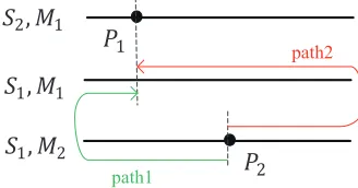
the same machine in two solutions S1 and S2, we define
do(S1, S2) = |PoS1 −PoS2| to be the difference of o be-tweenS1 andS2 (see Fig. 2). Otherwise,ocan be moved
to the beginning (end) of MS1
o , and then from the begin-ning (end) ofMS2
o ofS1to the same position as inMoS2 of
S2(see path1 (path2) in Fig. 3). The minimum one between
path1 and path2 is chosen as the difference ofobetweenS1
andS2, which isdo(S1, S2) = min{PoS1+P S2 o ,(L
S1 MS1
o
−
PS1 o ) + (L
S2 MS2
o
−PS2
o )}. Then, the distance betweenS1and
S2is defined asd(S1, S2) =P
n i=1
Pm
j=1doij(S1, S2).
Therefore, in order to obtainTi+1 fromTi, our path
re-linking applies a single move that changes the position of an operation on the same machine or re-assigns a different ma-chine to an operation, such that the resulted solution is feasi-ble and closer toS2thanTi. Note that the moved operation
can be non-critical. Our neighborhood is in factNπ g ∪Ngk, where Nπ
g (Ngk) is extended from Nπ (Nk) by including the moves of non-critical operations resulting in feasible so-lutions. This path relinking is much simpler thanks to the unique distance.
Algorithm 2 presents our recombination operator based on path relinking. The operator uses three parameters α,
β andγ, whose value will be established empirically later. The path from the initial solution Si to the guiding solu-tion Sg is built step by step as follows. LetSc be the cur-rent solution (Scis initialized to beSi). First, we construct the set of feasible solutions N that can be obtained from
Sc by applying a single move (lines 5–13). For each op-eration o, if o is on different machines in Sc and Sg, let
Nk
g(Sc, o) be the set of feasible solutions obtained from
Sc by movingoto the machine ofo inSg. Otherwise, let
Ngπ(Sc, o)be the set of feasible solutions obtained fromSc by changing the position of o on the same machine. Let
Algorithm 2A path relinking based recombination operator 1: Input: Initial solutionSiand guiding solutionSg
2: Output: A reference solutionSr
3: Sc←Si, P athSet← ∅,N← ∅
4: whiled(Sc, Sg)> α×d(Si, Sg)do 5: foreach operationoinScdo 6: ifMSc
o 6=M Sg
o then
7: Smin←arg min{do(S, Sg)|S∈Ngk(Sc, o)} 8: N ←N∪ {Smin}
9: else ifMSc
o =M Sg
o andPoSc6=P Sg
o then 10: Smin←arg min{do(S, Sg)|S∈Ngπ(Sc, o)} 11: N ←N∪ {Smin}
12: end if 13: end for
14: foreach solutionS∈Ndo
15: ifd(S, Sg)> d(Sc, Sg)then
16: N ←N\ {S}
17: else
18: estimate makespanobj(S) 19: end if
20: end for
21: foreach solutionS∈Ndo
22: indexDis(S)← |{T ∈N|d(T, Sg)< d(S, Sg)}| 23: indexObj(S)← |{T ∈N|obj(T)< obj(S)}| 24: end for
25: sortN in increasing order of indexDis(S)+indexObj(S), breaking ties randomly
26: k←rand{0,1, . . . ,min{γ,|N| −1}}
27: Sc←N(k);N← ∅
28: ifd(Sc, Sg)< β×d(Si, Sg)then
29: P athSet←P ahtSet∪ {Sc}
30: end if 31: end while
32: Sr= arg min{f(S), S∈P athSet},returnSr
(ties are broken randomly). Then, Smin in Ngk(Sc, o) or
Ngπ(Sc, o)is added intoN. Second, each solutionS such that d(S, Sg) > d(Sc, Sg) is removed from N, and the makespan of each remaining solution is estimated (lines 14– 18). Third, for each remaining solutionSinN, the number of solutions closer toSg (with a better makespan) is com-puted and is denoted by indexDis(S)(indexObj(S)) (lines 21–24). Note that indexDis(S)and indexObj(S)represent here two measures of quality for S. Fourth, we sort N in the increasing order of indexDis(S) +indexObj(S)and ran-domly choose one of the firstγsolutions to be the nextSc along the path, and store it inP athSetif its distance toSg is smaller thanβ×d(Si, Sg)(lines 25–30). These steps re-peats untild(Sc, Sg)is no longer larger thanα×d(Si, Sg) (line 4). Finally, the best solution inP athSetis returned as the reference solution (line 32).
It is obvious that the maximum size of setN isnowhere
no is the number of all the operations in all the jobs, i.e.,
no =P n
j=1nj. The worst time complexity of lines 5-13 is
O(n2o). Lines 21-25 are actually sorting the solutions of set
N, where the time complexity isO(|N|log|N|). Therefore, the worst time complexity of Algorithm 2 isO(n3
o).
Computational Results
Experimental protocol and benchmarks
Our MAE algorithm is implemented in C++ and runs on an Intel Xeon E5-2697 processor with 2.60 GHz CPU and 2 GB RAM. In our experiments, we setp, α, β, γ to 10, 0.4, 0.6, and 5, respectively. Two solutions are considered to be close and one of them is to be replaced with a random solution when the number of operations that have different machine assignments or different positions on the same machine is less than 10% of the total number of operations in all jobs. The maximum number of iterations of the tabu search pro-cedure is 10000. These parameter values are determined by extensive preliminary experiments.
We evaluate the performance of MAE on four bench-marks widely used in the literature:DPdata(Dauz`ere-P´er`es and Paulli 1997), BCdata (Barnes and Chambers 1998),
BRdata(Brandimarte 1993), andHUdata(Hurink, Jurisch, and Thole 1994), having 313 instances in total with differ-ent sizes and flexibilities. MAE is applied on each instance with 20 independent runs. Following the common practice in the field, we use the following values to compare dif-ferent methods: The average relative percentage deviation
RP D of objectives over the 20 runs defined asRP D = 100×(f −LB)/LB, wheref is the makespan obtained by a given algorithm, andLBis the lower bound provided in Quintiq1; and the average computational timet(s)in
sec-onds over the 20 runs.
In order to have a fair comparison with other algorithms, the cutoff time of MAE is set to 90 seconds for the BR-dataandBCdatainstances, and 5 minutes for theDPdata
andHUdatainstances, which is the same as that in GRASP-mELS. We also provide the results of MAE with a cutoff time of 1 hour. Besides, we normalize the computational time as the computer-independent CPU time (CI-CPU) in the same way as that in GRASP-mELS. Therefore, setting the speed factor of our computer as 1, the speed factor of GRASP-mELS, SSPR, HA, and HGTS are 1.09, 0.75, 0.50, and 0.63, respectively.
Comparison with metaheuristics
We compare our MAE algorithm with the recent state-of-the-art algorithms (SSPR, HGTS, HA, and GRASP-mELS) on the four benchmark sets. The comparative results are re-ported in Tables 1-4. Note that columns best (avg) and t(s) are the best (average) solutions obtained and average com-putational time in seconds required by each algorithm, the
LBvalues marked with∗denote the optimal solutions, and the best known solutions that can be obtained by each ref-erence algorithm are indicated in bold. Rows #better, #even, and #worse give the number of instances for which the best solutions obtained by MAE within 5 minutes or 90 seconds are better, equal, and worse than each reference algorithm.
1
Table 1: Comparison between MAE and other reference algorithms on theDPdatainstance set
Ins. LB
2015 2015 2016 2017 This paper This paper
SSPR HGTS HA GRASP-mELS MAE(5 min) MAE(1 hour)
best(avg) t(s) best(avg) t(s) best t(s) best(avg) t(s) best(avg) t(s) best(avg) t(s)
01a 2505∗ 2505(2508) 68 2505(2505) 122 2505 108 2505(2505) 62 2505(2505) 28.56 2505(2505) 28.56 02a 2228∗ 2229(2230) 100 2230(2234) 205 2230 133 2229(2231) 86 2228(2230.7) 145.12 2228(2229.9) 712.33 03a 2228∗ 2228(2228) 110 2228(2230) 181 2229 97 2228(2230) 94 2228(2228) 55.8 2228(2228) 55.8 04a 2503∗ 2503(2504) 57 2503(2503) 112 2503 87 2503(2503) 31 2503(2503) 8.62 2503(2503) 8.62 05a 2192 2211(2215) 112 2214(2218) 208 2212 116 2212(2215) 126 2208(2211.45) 125.69 2203(2208.05) 834.49 06a 2163 2183(2192) 181 2193(2198) 260 2197 93 2195(2200) 181 2182(2188.85) 177.42 2181(2184.3) 1867.14 07a 2216 2274(2285) 139 2270(2280) 344 2279 204 2276(2284) 127 2269(2274.6) 180.3 2254(2273.85) 2316.78 08a 2061∗ 2064(2066) 181 2070(2074) 318 2067 184 2069(2072) 144 2063(2064.3) 122.58 2062(2063.4) 1741.55 09a 2061∗ 2062(2063) 213 2067(2069) 376 2065 201 2069(2071) 170 2062(2063.15) 176.44 2062(2063.1) 472.62 10a 2212 2269(2287) 120 2247(2266) 369 2287 238 2263(2278) 110 2247(2266.4) 224.36 2245(2266.15) 2428.7 11a 2018 2051(2058) 193 2064(2069) 294 2060 181 2065(2068) 170 2050(2051.8) 200.57 2045(2049.75) 2865.49 12a 1969 2018(2020) 280 2027(2033) 486 2027 151 2039(2045) 148 2016(2021.45) 215.64 2008(2019.3) 1588.16 13a 2197 2248(2257) 119 2250(2264) 416 2248 293 2252(2263) 158 2247(2251.75) 116.55 2236(2246.65) 2674.32 14a 2161∗ 2163(2164) 269 2170(2173) 396 2167 210 2170(2174) 191 2163(2163.9) 191.26 2162(2163.2) 2915.81 15a 2161∗ 2162(2163) 376 2168(2169) 523 2163 192 2172(2174) 173 2162(2164.35) 203.2 2162(2163.15) 568.14 16a 2193 2244(2253) 131 2246(2257) 384 2249 160 2243(2258) 151 2242(2251.65) 196.5 2232(2245.45) 2135.66 17a 2088 2130(2134) 299 2142(2146) 483 2140 203 2145(2152) 190 2128(2132.7) 245.71 2121(2129.3) 1682.54 18a 2057 2119(2123) 409 2129(2133) 650 2132 133 2146(2151) 164 2118(2124.85) 242.2 2108(2114.6) 1752.68
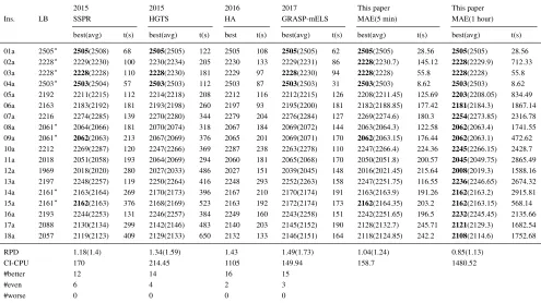
RPD 1.18(1.4) 1.34(1.59) 1.43 1.49(1.73) 1.04(1.24) 0.85(1.13)
CI-CPU 170 214.45 1105 149.94 158.7 1480.52
#better 12 14 16 15
#even 6 4 2 3
#worse 0 0 0 0
From Table 1, one observes that MAE outperforms HGTS, and HA in terms of both solution quality and compu-tational time on theDPdatabenchmark. Although it requires slightly more computational time than SSPR and GRASP-mELS, MAE has the least RP D values (1.04 and 1.24) for the best and average objective values. Besides, MAE obtains better results for 12 and 15 instances than SSPR and GRASP-mELS, respectively. When extending the cut-off time to 1 hour, MAE improves the previous best known solutions for 15 instances.
From Table 2, one observes that MAE is competitive with HGTS and HA on the BCdatabenchmark, because it has smaller values for the best and average objective values. Be-sides, MAE outperforms HGTS in terms of solution quality. Compared with SSPR, MAE obtains better, equal, and worse solutions for 1, 19, and 1 instances, respectively. GRASP-mELS has better performance than MAE on the BCdata
benchmark.
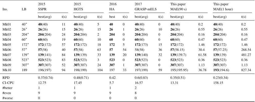
Results in Table 3 show that MAE outperforms SSPR, HGTS, and GRASP-mELS in terms of both solution quality and computational time onBRdata. Although HA requires slightly less computational time, MAE has smaller values for the best and average makespan. Besides, MAE obtains better or the same results for all the instances compared with other reference algorithms.
Table 4 presents the results of MAE in comparison with SSPR and GRASP-mELS on theHUdatabenchmark. One observes that MAE outperforms SSPR and GRASP-mELS because MAE obtains better or equal results for all the instances with less computational time only except for
GRASP-mELS on the rdata set. In particular, MAE im-proves the best results obtained by GRASP-mELS(SSPR) for 4(5), 18(19), and 13(9) instances on edata,rdata, and
vdata, respectively.
In sum, MAE improves the previous best results obtained by SSPR and GRASP-mELS for 47 and 52 out of the 178 test instances.
Comparison with the state-of-the-art exact method
We compare MAE with the state-of-the-art exact method based on constraint programming: LNS+FDS (Vil´ım, La-borie, and Shaw 2015). LNS+FDS constitutes the basis of the automatic search for scheduling problems in CP Opti-mizer, which is part of IBM ILOG CPLEX Optimization Studio. LNS+FDS (also denoted as CPO) has been success-fully tested on a range of scheduling benchmarks such as JSP and FJSP, etc.
MAE obtains better, equal, and worse results for 45, 255, and 13 instances compared with CPO among the 313 in-stances, respectively. Table 5 reports the results of MAE and comparison with CPO for the 45 improving instances. Note that the results of CPO were obtained with a time limit of 8 hours, while the results of MAE were obtained with a time limit of 1 hour.
Comparison with the industrial solver Quintiq
Table 2: Comparison between MAE and other reference algorithms on theBCdatainstance set
Ins. LB
2015 2015 2016 2017 This paper This paper
SSPR HGTS HA GRASP-mELS MAE(90 s) MAE(1 hour)
best(avg) t(s) best(avg) t(s) best t(s) best(avg) t(s) best(avg) t(s) best(avg) t(s)
mt10c1 927∗ 927(928) 26 927(927) 13 927 12 927(927) 8 927(927.3) 45.72 927(927) 61.69
mt10cc 908∗ 908(908) 20 908(910) 13 908 10 908(909) 17 908(909.85) 14.25 908(909.4) 125.5
mt10x 918∗ 918(918) 23 918(918) 15 918 11 918(918) 2 918(918) 25.67 918(918) 25.67
mt10xx 918∗ 918(918) 19 918(918) 12 918 11 918(918) 2 918(918) 4.5 918(918) 4.5
mt10xxx 918∗ 918(918) 20 918(918) 12 918 11 918(918) 2 918(918) 6.78 918(918) 6.78
mt10xy 905∗ 905(906) 21 905(905) 13 905 11 905(905) 26 905(905) 34.42 905(905) 34.42
mt10xyz 847∗ 847(847) 20 847(850) 18 847 9 847(847) 26 847(847.65) 35.46 847(847) 256.38
setb4c9 914∗ 914(916) 28 914(914) 16 914 15 914(914) 11 914(918.25) 39.78 914(914) 302.61
setb4cc 907∗ 907(907) 21 907(908) 15 907 15 907(907) 29 907(907) 12.54 907(907) 12.54
setb4x 925∗ 925(925) 19 925(925) 15 925 13 925(925) 4 925(925) 16.42 925(925) 16.42
setb4xx 925∗ 925(925) 21 925(925) 14 925 5 925(925) 2 925(925) 7.7 925(925) 7.7
setb4xxx 925∗ 925(925) 22 925(925) 15 925 9 925(925) 3 925(925) 8.45 925(925) 8.45
setb4xy 910∗ 910(912) 32 910(910) 19 910 12 910(910) 18 910(910) 58.79 910(910) 58.79
setb4xyz 902∗ 905(905) 21 905(905) 15 905 14 902(904) 11 902(905.6) 34.6 902(903.55) 956.86 seti5c12 1169∗ 1170(1173) 25 1170(1171) 41 1170 31 1169(1172) 39 1170(1174.4) 64.13 1170(1173.2) 205.68 seti5cc 1135∗ 1135(1136) 29 1136(1137) 34 1136 17 1135(1136) 24 1135(1136.2) 32.41 1135(1135.65) 243.52 seti5x 1198∗ 1198(1199) 41 1199(1201) 38 1198 27 1198(1199) 36 1198(1201.6) 75.48 1198(1199.35) 341.4 seti5xx 1194∗ 1197(1199) 37 1197(1198) 34 1197 29 1194(1197) 26 1197(1198.5) 45.76 1197(1197) 473.48 seti5xxx 1194∗ 1194(1198) 38 1197(1198) 31 1197 19 1194(1197) 27 1197(1198.45) 35.5 1194(1196.7) 612.57 seti5xy 1135∗ 1135(1136) 29 1136(1137) 34 1136 17 1135(1136) 28 1135(1136.4) 25.53 1135(1136) 227.91 seti5xyz 1125∗ 1125(1126) 35 1125(1126) 43 1125 33 1125(1127) 42 1125(1128.75) 32.96 1125(1125.65) 336.27
RPD 0.03(0.12) 0.07(0.13) 0.05 0(0.07) 0.03(0.17) 0.02(0.08)
CI-CPU 12.75 13.8 7.88 19.88 31.28 205.67
#better 1 4 3 0
#even 19 17 18 18
#worse 1 0 0 3
Table 3: Comparison between MAE and other reference algorithms on theBRdatainstance set
Ins. LB
2015 2015 2016 2017 This paper This paper
SSPR HGTS HA GRASP-mELS MAE(90 s) MAE(1 hour)
best(avg) t(s) best(avg) t(s) best t(s) best(avg) t(s) best(avg) t(s) best(avg) t(s)
Mk01 40∗ 40(40) 11 40(40) 5 40 0 40(40) 0 40(40) 0.2 40(40) 0.2
Mk02 26∗ 26(26) 15 26(26) 15 26 1 26(26) 10 26(26) 0.55 26(26) 0.55
Mk03 204∗ 204(204) 24 204(204) 2 204 0 204(204) 0 204(204) 0.16 204(204) 0.16
Mk04 60∗ 60(60) 19 60(60) 10 60 0 60(60) 0 60(60) 0.47 60(60) 0.47
Mk05 172∗ 172(172) 57 172(172) 18 172 5 172(173) 15 172(172) 1.46 172(172) 1.46
Mk06 57∗ 57(58) 40 57(58) 63 57 54 58(58) 36 57(58.15) 30.4 57(57.25) 268.54
Mk07 139∗ 139(141) 84 139(139) 33 139 20 139(140) 32 139(139.7) 61.58 139(139) 481.27
Mk08 523∗ 523(523) 83 523(523) 3 523 0 523(523) 0 523(523) 0.36 523(523) 0.36
Mk09 307∗ 307(307) 52 307(307) 24 307 1 307(307) 0 307(307) 1.13 307(307) 1.13
Mk10 189 196(197) 94 198(199) 104 197 33 197(199) 59 195(195.95) 36.78 193(194.6) 827.34
RPD 0.37(0.74) 0.48(0.71) 0.42 0.6(0.83) 0.35(0.51) 0.23(0.34)
CI-CPU 12.75 17.45 5.7 16.57 13.31 158.15
#better 1 1 1 2
#even 9 9 9 8
#worse 0 0 0 0
records of solution quality for all the 313 instances, together with the first method to hit the records. However, Quintiq did not describe their methods and the time limits to obtain these results.
We compare MAE with Quintiq by using a time limit of 1 hour for MAE. Experiments show that MAE obtains better
Table 4: Comparison between MAE and other reference algorithms onHUdataw.r.t. RPD values
Ins.
edata rdata vdata
SSPR MAE(5 min) GRASP-mELS SSPR MAE(5 min) GRASP-mELS SSPR MAE(5 min)
best avg best avg best avg best avg best avg best avg best avg best avg
mt06/10/20 0 0.04 0 0.07 0 0 0 0 0 0 0 0 0 0 0 0
la01-la05 0 0 0 0 0 0.07 0.07 0.09 0 0.07 0 0 0 0 0 0
la06-la10 0 0 0 0 0 0 0 0.01 0 0 0 0 0 0 0 0
la11-la15 0 0 0 0 0 0 0 0 0 0 0 0 0 0 0 0
la16-la20 0 0 0 0 0 0 0 0.03 0 0 0 0 0 0 0 0
la21-la25 0.08 0.23 0 0.22 2.63 3.27 2.53 2.91 1.91 2.35 0.49 0.8 0.23 0.35 0.1 0.24
la26-la30 0.43 0.66 0.3 0.73 0.36 0.71 0.36 0.48 0.13 0.27 0.17 0.24 0.06 0.08 0 0.03
la31-la35 0.01 0.07 0 0.01 0.05 0.12 0.04 0.05 0 0.02 0.04 0.07 0.01 0.02 0 0
la36-la40 0 0.05 0 0.02 0.36 1.22 0.66 0.9 0 0.1 0 0 0 0 0 0
CI-CPU 18 51 34 44 30 47 25
#better 5 18 19 13 9
#even 38 25 24 30 34
#worse 0 0 0 0 0
Table 5: The improved results of MAE compared with CPO on 45 instances
Ins. CPO MAE Ins. CPO MAE
LB UB UB LB UB UB
Mk05 168 173 172 r-la23 816 832 831
Mk10 183 195 193 r-la24 775 805 795
02a 2228 2234 2228 r-la25 768 787 779
05a 2189 2213 2203 r-la26 1056 1066 1057
06a 2162 2191 2181 r-la27 1085 1099 1086
07a 2216 2277 2254 r-la28 1075 1079 1076
08a 2061 2066 2062 r-la29 993 1001 994
10a 2197 2263 2245 r-la30 1068 1089 1071
11a 2017 2067 2045 r-la31 1520 1522 1520
12a 1969 2013 2008 r-la32 1657 1658 1657
13a 2197 2258 2236 r-la33 1497 1498 1497
14a 2161 2163 2162 r-la34 1535 1536 1535
16a 2148 2240 2232 v-car1 5005 5006 5005
17a 2088 2140 2121 v-car3 5597 5599 5597
18a 2057 2125 2103 v-car5 4909 4912 4910
e-abz7 564 620 610 v-la22 733 734 733
e-abz8 586 639 636 v-la25 751 753 752
r-abz7 492 535 522 v-la29 993 994 993
r-abz8 506 558 535 v-la30 1068 1069 1068
r-abz9 497 553 536 v-la32 1657 1658 1657
r-car3 5597 5623 5622 v-la33 1497 1498 1497
r-la21 808 838 825 v-la35 1549 1550 1549
r-la22 741 755 753
is reported in Table 7, where columns<,=, and>denote the number of instances that MAE obtains better, equal, and worse results than the reference algorithms.
Discuss and analysis
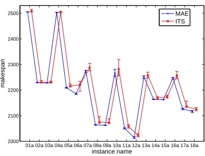
To show the merit of the two-individual based evolutionary framework, we compare MAE with the trajectory method called iterated tabu search (ITS) which works on a single
Table 6: New world records obtained by MAE
Ins. Previous world record MAE
LB LB
Ref.
UB UB
Ref.
UB Date UB
05a 2192 [Q] 2204 [Q] Nov. 2015 2203
07a 2216 [CPO] 2264 [Q] Nov. 2015 2254
13a 2197 [CPO] 2239 [Q] Jan. 2016 2236
rdata-abz7 493 [Q] 524 [Q] Jan. 2016 522
rdata-abz8 507 [Q] 536 [Q] Jan. 2016 535
rdata-la22 741 [CPO] 755 [CPO] Nov. 2013 753 rdata-la23 816 [Q] 832 [CPO] Mar. 2013 831
rdata-la24 775 [Q] 796 [Q] Nov. 2015 795
rdata-la25 768 [CPO] 783 [Q] Jan. 2016 779 vdata-car5 4909 [Q] 4911 [Q] Nov. 2015 4910
Table 7: Summary of MAE compared with CPO and Quintiq
Set MAE(1 h) vs CPO(8 h) MAE(1 h) vs Quintiq
< = > < = >
DPdata 13 5 0 3 2 10
BCdata 0 18 3 0 0 0
BRdata 2 8 0 0 2 0
HUdata
edata 2 60 4 0 20 0
rdata 18 48 0 6 30 1
vdata 10 53 3 1 22 0
sdata 0 63 3 0 18 6
Total 45 255 13 10 94 17
01a 02a 03a 04a 05a 06a 07a 08a 09a 10a 11a 12a 13a 14a 15a 16a 17a 18a 2000
2100 2200 2300 2400 2500
instance name
makespan
MAE ITS
Figure 4: Comparison between MAE and ITS onDPdata.
Fig. 4 shows the best, average, and worst solutions ob-tained by MAE and ITS for each of the 18 instances in DP-data. It can be observed that the best, average, and worst solutions of MAE are better than or equal to those of ITS for all the instances. Besides, the differences between the best and worst solutions of MAE are also smaller than those of ITS. This indicates that the two-individual based evolution-ary algorithm is superior to the trajectory method.
In the preliminary experiments, we have taken 11 differ-ent values (5, 6, . . . ,15) ofp, 5 different groups of values ([0, 0.2], . . . , [0.8, 1]) of[α, β], and 10 different values (1, . . . ,10) ofγto analyze the parameter sensitivity. There are totally 11 * 5 * 10 = 550 combinations for all the parameters. We ran MAE 10 times independently to solve a relatively difficult instance seti5xyz in BCdatawith each of the 550 combinations, the cutoff time of each run being 90 seconds. The results show that MAE achieves the best performance whenp,α,β, andγ are set to 10, 0.4, 0.6, and 5, respec-tively, considering both solution quality and computational efficiency. In the following paragraphs, we will further an-alyze the impact of one parameter on the performance of MAE by extending its value domain and keeping other pa-rameters fixed.
To analyze the impact of parameterpon the performance of MAE, we take 20 different values (p ∈ {1, . . . ,20}), keep other parameters fixed, and apply MAE on all the in-stances inDPdata. The corresponding results are plotted in Fig. 5. One finds that the average makespan decreases when
p ∈ {1, . . . ,10}and keeps flat or slightly increases when
p∈ {10, . . . ,20}, while the computational time drastically decreases whenp∈ {1,2,3}and gradually increases when
p∈ {3, . . . ,20}. The reason might lie in the fact that when
pis small, the best solution preserved in the previous cycle is not of high quality, which cannot provide good features to be inherited. When pis too large, the best solution in a cycle is closer to the best solution found so far, which can-not provide sufficient diversity, so that MAE would be more likely trapped into local optima. The best value ofpin MAE is suggested to be 10.
0 5 10 15 20
2199 2202 2205 2208 2211
value of p
average makespan
138 150 162 173
average computational time
best makespan average makespan average computational time
Figure 5: The average makespan and computational time corresponding to different values of parameterponDPdata.
[0, 0.2] [0.2, 0.4] [0.4, 0.6] [0.6, 0.8] [0.8, 1]
2100 2150 2200 2250 2300
value of parameter [α, β]
average makespan
0 40 80 120 160 200
average computational time
average makespan avearge computational time
Figure 6: The average makespan and computational time corresponding to different values of parameter[α, β]on DP-data.
To analyze the impact of the parametersα, β, γon MAE, we take 5 groups of values ([0,0.2], . . . ,[0.8,1]) for[α, β], 15 values (1, . . . ,15) for γ, keep other parameters fixed, and conduct experiments on DPdata and BCdata, respec-tively. The results are presented in Fig. 6 and Fig. 7. Fig. 6 shows that the average makespan decreases from the first to the third group and increases from the third to the fifth group, while the corresponding computational time gradu-ally increases in the whole range. Fig. 7 shows that both average makespan and computational time decrease when
γ ∈ {1, . . . ,5} and increase whenγ ∈ {5, . . . ,15}. Con-sidering both solution quality and computational efficiency,
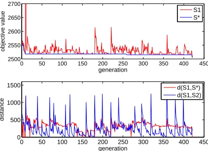
α, β, γare suggested to be 0.4, 0.6, and 5, respectively. MAE is effective because it maintains a good balance be-tween intensification and diversification using two individu-alsS1andS2, whereS1plays the role of intensification and
S2plays the role of diversification. To illustrate this, we
0 5 10 15
997 998 999
value of parameter γ
average makespan
10 20 30 40 50 60
average computational time
average makespan average computational time
Figure 7: The average makespan and computational time corresponding to different values of parameterγonBCdata.
0 50 100 150 200 250 300 350 400 450
2500 2550 2600 2650 2700
generation
objective value
S1 S*
0 50 100 150 200 250 300 350 400 450
0 500 1000 1500
generation
distance
d(S1,S*) d(S1,S2)
Figure 8: The evolution of objective values and distances when solving instance01a.
S∗ which is the best S1 obtained so far, and the distances
d(S1, S∗)andd(S1, S2)when solving the representative
in-stance01a. We see that the objective value ofS1is generally
good and that ofS∗is monotonously improved. This is pos-sible because d(S1, S2) periodically becomes large
(com-paring withd(S1, S∗)), so that the path relinking operator
onS1andS2is able to find diversified solutions.
Furthermore, we apply statistical significance test on the average makespan of the instances which are obtained by multiple runs of MAE compared with SSPR and GRASP-mELS, the resulting p-value of the average makespan be-tween MAE and SSPR (GRASP-mELS) are reported in Ta-ble 8. Considering a level of significance of 0.05, one ob-serves from Table 8 that there is significant difference be-tween MAE and SSPR on DPdata, rdata, and vdata, and there is no significant difference between MAE and SSPR onBCdata,BRdata, andedata. Besides, there is significant difference between MAE and GRASP-mELS on DPdata,
rdata, vdata, and BCdata, and there is no significant dif-ference between MAE and GRASP-mELS onBRdataand
Table 8: Statistical significance test
Benchmark set MAE vs. SSPR MAE vs. GRASP-mELS
DPdata 4.79×10⁻² 3.28×10⁻⁵ rdata 1.3×10⁻⁴ 6.17×10⁻⁵ vdata 2.13×10⁻³ 3.69×10⁻⁴ BCdata 8.37×10⁻² 7.12×10⁻³
BRdata 0.2066 0.2230
edata 0.7746 0.7724
edata. The reason may lie in the fact that the instances in
BCdata,BRdata, andedataare relatively easy to solve. The values of #better, #even, and #worse in Tables 1-4 also give an idea of the difficulties of the instances.
Conclusion
We have proposed a master-apprentice evolutionary algo-rithm called MAE for solving the flexible job shop schedul-ing problem, which distschedul-inguishes itself from both sschedul-ingle solution-based and traditional population-based metaheuris-tics in three main aspects: (1) The population size in MAE is two, allowing effective collaboration between the two indi-viduals; (2) MAE uses a simple but very effective individual updating strategy to ensure the quality and the diversity of the evolution; (3) In order to generate promising offspring solutions, MAE uses a semantic problem-specific recombi-nation operator based on path relinking with a novel distance definition for two individuals. Computational experiments show the high performance of MAE in terms of both solu-tion quality and computasolu-tional efficiency. We strongly be-lieve that this two-individual based mater-apprentice evolu-tionary algorithm is a promising framework for solving other challenging combinatorial optimization problems.
Acknowledgments
The research was supported by China Postdoctoral Sci-ence Foundation funded project under grant number 2018M630861 and National Natural Science Foundation of China under grant numbers 61370183 and 71320107001 .
References
Barnes, J. W., and Chambers, J. B. 1998. Flexible job shop schedul-ing by tabu search. Technical report, The University of Texas at Austin.
Bo˙zejko, W.; Uchro´nski, M.; and Wodecki, M. 2010. Parallel hy-brid metaheuristics for the flexible job shop problem. Computers and Industrial Engineering59(2):323–333.
Brandimarte, P. 1993. Routing and scheduling in a flexible job shop by tabu search.Annals of Operations Research41(3):157–183. Brucker, P., and Schlie, R. 1991. Job-shop scheduling with multi-purpose machines. Springer-Verlag New York, Inc.
Dauz`ere-P´er`es, S., and Paulli, J. 1997. An integrated approach for modeling and solving the general multiprocessor job-shop schedul-ing problem usschedul-ing tabu search. Annals of Operations Research
70(1):281–306.
max-cut problem. InProceedings of the 7th Annual Conference on Genetic and Evolutionary Computation, GECCO ’05, 999–1006. New York, NY, USA: ACM.
Gao, K.-Z.; Suganthan, P. N.; Pan, Q.-K.; Chua, T. J.; Cai, T.-X.; and Chong, C.-S. 2016. Discrete harmony search algorithm for flexible job shop scheduling problem with multiple objectives.
Journal of Intelligent Manufacturing27(2):363–374.
Gao, J.; Sun, L.; and Gen, M. 2008. A hybrid genetic and variable neighborhood descent algorithm for flexible job shop scheduling problems.Computers & Operations Research35(9):2892–2907. Garey, M. R.; Johnson, D. S.; and Sethi, R. 1976. The complexity of flowshop and jobshop scheduling. Mathematics of Operations Research1(2):117–129.
Gomes, M. C.; Barbosa-Pvoa, A. P.; and Novais, A. Q. 2013. Reac-tive scheduling in a make-to-order flexible job shop with re-entrant process and assembly: a mathematical programming approach. In-ternational Journal of Production Research51(17):5120–5141. Gonz´alez, M. A.; Vela, C. R.; and Varela, R. 2013. An efficient memetic algorithm for the flexible job shop with setup times. In In-ternational Conference on InIn-ternational Conference on Automated Planning and Scheduling, 91–99.
Gonz´alez, M. A.; Vela, C. R.; and Varela, R. 2015. Scatter search with path relinking for the flexible job shop scheduling problem.
European Journal of Operational Research245(1):35–45. Guti´errez, C., and Garc´ıa-Magari˜no, I. 2011. Modular design of a hybrid genetic algorithm for a flexible jobshop scheduling problem.
Knowledge-Based Systems24(1):102–112.
Hansmann, R. S.; Rieger, T.; and Zimmermann, U. T. 2014. Flexi-ble job shop scheduling with blockages.Mathematical Methods of Operations Research79(2):135–161.
Hmida, A. B.; Haouari, M.; and Lopez, P. 2010. Discrepancy search for the flexible job shop scheduling problem.Computers & Operations Research37(12):2192–2201.
Hurink, J.; Jurisch, B.; and Thole, M. 1994. Tabu search for the job-shop scheduling problem with multi-purpose machines.
Operations-Research-Spektrum15(4):205–215.
Kemmo´e-Tchomt´e, S.; Lamy, D.; and Tchernev, N. 2017. An effec-tive multi-start multi-level evolutionary local search for the flexible job-shop problem. Engineering Applications of Artificial Intelli-gence62:80–95.
Lahiri, M., and Cebrian, M. 2010. The genetic algorithm as a gen-eral diffusion model for social networks. InTwenty-Fourth AAAI Conference on Artificial Intelligence, 494–499.
Li, X., and Gao, L. 2016. An effective hybrid genetic algorithm and tabu search for flexible job shop scheduling problem.International Journal of Production Economics174:93–110.
Li, J.-Q.; Pan, Q.-K.; and Liang, Y.-C. 2010. An effective hybrid tabu search algorithm for multi-objective flexible job-shop schedul-ing problems. Computers & Industrial Engineering 59(4):647– 662.
L¨u, Z.; Glover, F.; and Hao, J. K. 2010. A hybrid metaheuris-tic approach to solving the UBQP problem. European Journal of Operational Research207(3):1254–1262.
Mastrolilli, M., and Gambardella, L. M. 2000. Effective neigh-borhood functions for the flexible job shop problem. Journal of Scheduling3(1):3–20.
Moalic, L., and Gondran, A. 2017. Variations on memetic algo-rithms for graph coloring problems.Journal of Heuristics1–24. Oddi, A.; Rasconi, R.; Cesta, A.; and Smith, S. F. 2011. Itera-tive flattening search for the flexible job shop scheduling problem.
InInternational Joint Conference on Artificial Intelligence, 1991– 1996.
¨
Ozg¨uven, C.; ¨Ozbakr, L.; and Yavuz, Y. 2010. Mathematical mod-els for job-shop scheduling problems with routing and process plan flexibility.Applied Mathematical Modelling34(6):1539–1548. Palacios, J. J.; Gonz´alez, M. A.; Vela, C. R.; Gonz´alez-Rodr´ıguez, I.; and Puente, J. 2015. Genetic tabu search for the fuzzy flexible job shop problem. Computers & Operations Research54(C):74– 89.
Peng, B.; L¨u, Z.; and Cheng, T. C. E. 2015. A tabu search/path re-linking algorithm to solve the job shop scheduling problem. Com-puters & Operations Research53(53):154–164.
Pezzella, F.; Morganti, G.; and Ciaschetti, G. 2008. A genetic algorithm for the flexible job-shop scheduling problem.Computers & Operations Research35(10):3202–3212.
Roshanaei, V.; Azab, A.; and Elmaraghy, H. 2013. Mathematical modelling and a meta-heuristic for flexible job shop scheduling.
International Journal of Production Research51(20):6247–6274. Sutton, A. M., and Neumann, F. 2012. A parameterized run-time analysis of evolutionary algorithms for the euclidean travel-ing salesperson problem. InAAAI Conference on Artificial Intelli-gence, 595 – 628.
Thomalla, C. 2005. Job shop scheduling with alternative process plans. International Journal of Production Economics74(1):125– 134.
Vil´ım, P.; Laborie, P.; and Shaw, P. 2015. Failure-directed search for constraint-based scheduling. InInternational Conference on AI and OR Techniques in Constraint Programming for Combinatorial Optimization Problems, 437–453.
Wang, L.; Zhou, G.; Xu, Y.; Wang, S.; and Liu, M. 2012. An effective artificial bee colony algorithm for the flexible job-shop scheduling problem. International Journal of Advanced Manufac-turing Technology56(60):1–8.
Wang, L.; Zhou, G.; Xu, Y.; and Liu, M. 2013. A hybrid artificial bee colony algorithm for the fuzzy flexible job-shop scheduling problem.International Journal of Production Research
51(12):3593–3608.
Yu, Y.; Yao, X.; and Zhou, Z.-H. 2013. On the approximation ability of evolutionary optimization with application to minimum set cover. InProceedings of the Twenty-Third International Joint Conference on Artificial Intelligence, 3190–3194. AAAI Press. Yuan, Y., and Xu, H. 2013a. Flexible job shop scheduling using hybrid differential evolution algorithms. Computers & Industrial Engineering65(2):246–260.