Heuristic Search Algorithm for Dimensionality Reduction Optimally Combining Feature Selection and Feature Extraction

(1)

The Thirty-Third AAAI Conference on Artificial Intelligence (AAAI-19)

Heuristic Search Algorithm for Dimensionality Reduction

Optimally Combining Feature Selection and Feature Extraction

Baokun He, Swair Shah, Crystal Maung, Gordon Arnold, Guihong Wan, Haim Schweitzer

(Baokun.He, swair, gordon.arnold, Guihong.Wan, HSchweitzer )@utdallas.edu, [email protected]

Department of Computer Science, The University of Texas at Dallas 800 W. Campbell Road, Richardson, TX 75080

Abstract

The following are two classical approaches to dimensionality reduction: 1. Approximating the data with a small number of features that exist in the data (feature selection). 2. Approx-imating the data with a small number of arbitrary features (feature extraction). We study a generalization that approxi-mates the data with both selected and extracted features. We show that an optimal solution to this hybrid problem involves a combinatorial search, and cannot be trivially obtained even if one can solve optimally the separate problems of selection and extraction. Our approach that gives optimal and approx-imate solutions uses a “best first” heuristic search. The algo-rithm comes with both ana prioriand ana posteriori opti-mality guarantee similar to those that can be obtained for the classical weighted A* algorithm. Experimental results show the effectiveness of the proposed approach.

1 Introduction

The representation of data in terms of a small number of features is a fundamental tool in data analysis. The compact representation allows for efficient manipulation, and may re-veal relations in the data that are harder to identify. We study the unsupervised case, where a typical criterion of quality for the representation is the accuracy with which the data can be reconstructed from the compact representation.

Letmbe the number of data items, each specified in terms ofnfeatures, so that the data can be viewed as the matrixX

ofmrows andncolumns. A compact representation withr

features is given by a matrixV of sizem×r, withr≤n. The reconstruction ofX fromV is computed byX ≈V A, whereAis ther×ncoefficients matrix. We note that the matrix V Ais of rank r, so thatX is being approximated by a rank rmatrix. Conversely, any rank r matrix can be expressed as the productV A, and thus gives a compact rep-resentation in terms ofrfeatures.

1.1 Previous work and the current state of the art

Studies of dimensionality reduction distinguish between the case where the columns ofV must also be columns ofX

(feature selection), and the case in which this constraint is not enforced (feature extraction). We review these two ap-proaches and then propose to combine them. We show that

Input: the matrixX, the integerr.

Output: thervectorsv1, . . . , vr.

1 Compute the matrixB=XXT.

2 v1, . . . , vrare the topreigenvectors ofB.

Figure 1: The algorithm for optimal feature extraction

applying selection followed by extraction or vice versa does not give the optimal hybrid representation.

LetΘbe a matrix norm, then the error of approximating the matrixXbyV Ais given by:

X ≈V A, error= Θ(X−V A) (1)

Feature extraction. The well-known algorithm for opti-mal feature extraction is shown in Fig.1. See, e.g., (Jolliffe 2002; Li et al. 2017). Applications of this algorithm include the technique of principal component analysis (PCA), which is arguably the most popular feature extraction technique. With recent advances in numerical techniques for comput-ing eigenvectors (e.g., (Halko, Martinsson, and Tropp 2011; Li et al. 2017)) the algorithm in Fig.1 can be implemented efficiently even for large amounts of data.

Among the topics of current research are attempts to min-imize the approximation error (1) in norms that are not uni-tarily invariant. This turns out to be very challenging. In particular, minimizing the entry-wisel1 orl0 norms is ex-pected to improve the robustness of the estimation, but un-fortunately the problem formulated in these norms turns out to be NP-hard. See, e.g., Gillis (2018), Song (2017), and Bringmann (2017). For the more general case of entrywise

lpnorms see Chierichetti (2017).

Feature selection. In feature selection the columns ofV

are constrained to be columns of X. This is sometimes known as the Column Subset Selection Problem (CSSP). See, e.g. (Golub and Van-Loan 2013). Even though the approximation obtained by feature selection is worse than the approximation obtained by feature extraction, there are advantages of feature selection that make it the preferred choice in many situations. For example:

(2)

the underlying data” (Drineas, Mahoney, and Muthukrish-nan 2008).

• Selected features generalize better than extracted fea-tures in machine learning tasks (Guyon and Elisseeff 2003).

• Functions computed from extracted features depend on all the features and are typically more expensive to evaluate than functions computed from few selected features.

• Feature selection retains the data sparsity.

To describe current and previous results we need the fol-lowing notation. LetEFE, EFSbe the smallest errors

obtain-able by feature extraction and by feature selection respec-tively. Consider an algorithm α that produces a selection

S from the matrix X. Its error is given by Eα(S, X) = minAΘ(X−SA). For such algorithm one can define:

pα(X) =

Eα(S, X)

EFE

, pα= max

X pα(X)

Then the value ofpαindicates the estimation quality in the

worst-case (e.g., Boutsidis (2009), Golub (2013)). The moti-vation behind this definition is that for any algorithmαand a matrixXwe have:1≤ Eα(S,X)

EFE ≤pα. Therefore, small

val-ues ofpαimply better worst-case performance. For example,

Deshpande (2010) showed that for the Frobenius norm error in selectingrfeaturespα =

√

r+ 1. Thus, we say that an algorithmαis optimal ifEα(S, X)is the smallest possible,

and it is worst-case optimal if itspαis the smallest possible.

Unsupervised feature selection formulated as CSSP has attracted a lot of attention, with the first algorithm (pivoted QR) being developed more than 50 years ago (Businger and Golub 1965). Recent results improve the accuracy, the run-ning time, and the number of passes (e.g., (Paul, Magdon-Ismail, and Drineas 2015; Maung and Schweitzer 2013)). The problem was recently proved NP-hard (Shitov 2017). There are, however, polynomial algorithms that are worst-case optimal, and nontrivial optimal algorithms that run much faster than exhaustive search.

Numerical linear algebra studies focus on algorithms for minimizing the Spectral norm. The deterministic algorithm with the best worst-case error can be found in (Gu and Eisenstat 1996). A randomized algorithm with an improved worst-case accuracy for the Spectral norm is described in (Boutsidis, Mahoney, and Drineas 2009). The theoretical computer science community produced worst-case optimal and near optimal randomized algorithms for the Frobenius norm. These include, among others, (Deshpande et al. 2006; Guruswami and Sinop 2012). A worst-case optimal deter-ministic algorithm for the Frobenius norm is given in (Desh-pande and Rademacher 2010; Guruswami and Sinop 2012). The algebraic approach taken by most researchers was shown effective in deriving worst-case optimal algorithms, but so far has not produced optimal algorithms. Recent stud-ies using classical AI tools of combinatorial search were used to derive optimal and near optimal algorithms in the Frobenius norm. See Arai (2015; 2016).

Hybrid low rank representation. As discussed above feature extraction and feature selection each have unique ad-vantages and disadad-vantages. A hybrid representation that in-cludes both extracted and selected features was previously

proposed in (Kneip and Sarda 2011) and (Wang 2012). The main idea is that feature extraction works well in situations where the features are highly correlated, while feature selec-tion works well in situaselec-tions where the data is uncorrelated. Therefore, these studies apply feature extraction to remove the correlated components and follow it by feature selection. As we show this approach is not optimal.

1.2 Our results

In our model we fix both the number of selected features and the number of extracted features, and attempt to perform se-lection and extraction to minimize the approximation error in various norms. We show that the optimal combination of extraction and selection cannot be obtained by separate op-timal algorithms for selection and extraction and requires a combinatorial search. To the best of our knowledge we are the first to make this observation.

The model we propose has r1 selected features and r2 extracted features. The approximation ofX is given by:

X≈SA1+V A2, error= min

A1,A2

Θ(X−SA1−V A2) (2)

whereSconsists ofr1columns fromXand ther2columns ofV are unconstrained. We refer to the representation in (2) as the “Hybrid Low Rank”, orHLR. Our main result is an al-gorithm that computes HLR for any unitarily invariant error criteria. Observe that the HLR has simple feature extraction and simple feature selection as special cases.

The algorithm. An obvious approach to obtain a hybrid low rank representation is to start with the selection of r1 features and follow it with the extraction ofr2features. An-other alternative is to have the order of selection and extrac-tion reversed. However, it turns out (see Secextrac-tion 2.1) that

neither of these approaches is optimal. Instead, we propose to use variants of a “best first” heuristic search to find opti-mal and near optiopti-mal HLR solutions.

The algorithm that we develop is based on the combina-torial approach to feature selection described in Arai (2016). The authors define a search graph for subsets, and use vari-ants of A* to find a solution. The key to their algorithm is the introduction of heuristic functions that use eigenvalues. We show that the solution to the HLR can be found in a similar way, but with different heuristic functions.

The main contributions.

• A heuristic search algorithm for computing optimal and near optimal hybrid low rank (HLR).

• A priorianda posterioribounds for these algorithms.

• Since feature selection is a special case of the HLR (r2=0), our HLR algorithm can also be used for optimal feature selection in all unitarily invariant norms. In partic-ular this gives the first optimal feature selection algorithm for the spectral norm and for the nuclear norm.

(3)

writeA ⊂ B to indicate that the columns ofAare a sub-set of the columns of B. We write |A| for the number of columns in A, and [A|B] for the matrix consisting of the columns ofAfollowed by the columns ofB.

Let Θbe an error criterion. We consider the following approximation errors:

EFE(X, r) = min

V,AΘ(X−V A)

subject to|V|=r EFS(X, r) = min

S,AΘ(X−SA)

subject toS⊂X,|S|=r EHLR(X, r1, r2) = min

S,A1,V,A2

Θ(X−SA1−V A2)

subject toS⊂X,|S|=r1,|V|=r2

(3)

From (3) it easily follows that withr=r1+r2we have:

EFE(X, r)≤EHLR(X, r1, r2)≤EFS(X, r) (4)

Thus, one would expect the HLR to have some desired erties of feature selection combined with some desired prop-erties of feature extraction. For example,r1of the HLR fea-tures are easy to interpret (as in feature selection), and only

r2of them are hard to interpret (as in feature extraction).

2.1 Greedy HLR is not Optimal

Suppose we are given a black box algorithm that computes optimal selection, and another black box algorithm that com-putes optimal extraction. We show by example that one can-not perform optimal selection followed by optimal extrac-tion, or vice versa, to compute the optimal HLR. Consider the following two matrices:

X1=

100 0 1

0 1 100

0 100 50

!

, X2=

20 0 12

−5 0 100

10 30 0

!

The goal for both matrices is to optimally select one column and extract one feature (r1= 1, r2= 1). If optimal selection of one feature is applied toX1, the best selection (in Frobe-nius norm) is Column 3 (the error is EFS(X1,1)=133.9). Combining the selection of Column 3 with an optimally ex-tracted single feature reduces the error to 89.0. This, how-ever, is not optimal. The selection of Column 1 with one extracted feature reduces the error to EHLR(X1,1,1)=77.4 which is optimal. This shows that optimal selection followed by optimal extraction does not guarantee the optimal HLR.

Similarly, if optimal extraction of one feature is applied toX2 followed by optimal selection, the error is reduced to 20.44. The selection in this case is Column 2. This is not optimal since it is possible to extract a feature fol-lowed by the selection of Column 3 and reduce the error toEHLR(X2,1,1)=18.8. This shows that optimal extraction followed by optimal selection does not guarantee the opti-mal HLR.

3 HLR by heuristic search

A recent paper (Arai et al. 2016) has shown how to solve CSSP with the weighted A* algorithm for the Frobenius

{}

{x1} {x2} {x3}

{x1, x2} {x1, x3} {x2, x3}

{x1, x2, x3}

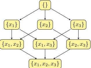
Figure 2: Example of the subsets graph

norm. They create a graph of subsets and perform the search on that graph. We use the same graph to convert the HLR into a graph search problem and study the performance of graph search algorithms for this problem. We propose two heuristics in a standard “best-first” setting. The first heuris-tic, that we call u, is an upper bound on the optimal HLR value. As we show, selecting graph nodes according to u

gives a fast greedy algorithm.

The second heuristic, that we call f, is a lower bound on the optimal HLR value. We prove that using f by it-self gives an algorithm that is guaranteed to find the optimal solution. Experimental results show that the algorithm runs much faster than exhaustive search (and produces the same results).

We linearly combine f and u to create the following heuristic:f0 =f +u. This gives a much faster algorithm than usingf by itself. This is similar to the weighted A* approach, and we prove that the solution found by our algo-rithm comes with guaranteed bounds on its accuracy.

3.1 The subsets graph

The subsets graph is created with nodes corresponding to column subsets. There is an edge from subsetSito subsetSj

if adding one column toSicreatesSj. The graph generated

for the matrixX = (x1, x2, x3)is shown in Fig.2.

Even though a subset graph is not a tree, it has two erties that are typically associated with trees. The first prop-erty is that it has a root, corresponding to the empty sub-set. The second is that all paths leading from the root to a node can be considered equivalent. For example, if the goal node{x1, x3} is found, it is irrelevant if it is reached by the path{} → {x1} → {x1, x3}or by the path{} →

{x3} → {x1, x3}. This is similar to the case of a tree where the choice of path leading to a node is irrelevant since there is a unique path leading from the root to any node.

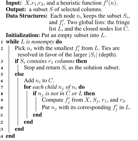
3.2 The heuristic search algorithm

The algorithm in Figure 3 performs the search for the opti-mal HLR. It is similar to the standard “best-first” algorithm except for the following notable difference. The standard graph search algorithm updates a node in the fringe if a bet-ter path to it is found (in Line 8 of the algorithm, whennj

(4)

Input: X,r1,r2, and a heuristic functionf0(n).

Output: a subsetSof selected columns.

Data Structures: Each nodenikeeps the subsetSi,

andfi0. Two global lists: the fringe

listL, and the closed nodes listC. Initialization:Put an empty subset intoL.

1 whileLis nonemptydo

2 Pickniwith the smallestfi0fromL. Ties are

resolved in favor of the larger|Si|(depth).

3 ifS_icontainsr1columnsthen

4 Stop and returnSias the solution subset.

5 else

6 AddnitoC.

7 foreach childnjofnido

8 ifnjis not inCorLthen

9 Computef_j0fromX,Sj,r1, andr2. 10 Putnjwith its correspondingfj0inL.

11 end

12 end

13 end

14 end

Figure 3: The best-first search algorithm.

As explained in Section 3.1, all paths to the same subset are equivalent, and the value of the node depends only on the subset and not on the path leading to the subset.

3.3 Heuristic functions

The HLR is defined in terms ofX, r1, r2. At each nodeni

the subsetSi and its sizeki =|Si|are known. Recall that

the errorEHLRis the smallest error of approximatingX by

a selection ofr1columns and the best possible additionalr2 unconstrained vectors. The functiondiat nodeniis defined

as the smallest error of approximatingXby a selection ofr1 columns that includeSiand the best possible additionalr2 unconstrained vectors. This is the value at the best goal node belowni. The functionuiat nodeniis defined as the

small-est error of approximatingXby the selectionSiand the best

possible additionalr2 unconstrained vectors. The function

fiat nodeniis defined as the smallest error of

approximat-ingX by the selectionSi and the best possible additional

r1+r2−kiunconstrained vectors, whereki=|Si|.

EHLR(X, r1, r2) = min

S,A1,V,A2

Θ(X−SA1−V A2)

subject to S⊂X,|S|=r1,|V|=r2

di =d(ni, r1, r2) = min

S,A1,V,A2

Θ(X−SA1−V A2)

subject to Si⊂S⊂X,|S|=r1,|V|=r2

ui=u(ni, r2) = min

A1,V,A2

Θ(X−SiA1−V A2)

subject to |V|=r2

fi=f(ni, r1, r2) = min

A1,V,A2

Θ(X−SiA1−V A2)

subject to |V|=r1+r2−ki

(5)

Observe that EHLR and di cannot be calculated efficiently

since the optimal selection S is unknown. By contrast,

ui and fi use only the partial selection available at the

given node, and as shown later can be computed efficiently. Clearly, the best heuristic choice for the algorithm isf_i0 =

di. But since it cannot be efficiently calculated we consider

other choices usingfiandui. The motivation behind these

choices is that bothfiandui can be viewed as

approxima-tions ofdi, as shown in Proposition 1.

Proposition 1: For each nodeni:

f(ni, r1, r2)≤d(ni, r1, r2)≤u(ni, r2)

and at a goal node (whereki=r1) the inequalities become equalities.

Proof:

• To see thatfi ≤ di observe that both fi anddi use the

same number of vectors (r1+r2), and both use the ki

vectors inSi. The rest of the vectors are unconstrained in

fibut partially constrained indi. This proves the left hand

side inequality.

• To see thatdi ≤ ui, letSi, V be the vector subsets that

are used to calculateui. The minimum in the definition of

diincludes the subsetsSiandV (and additional vectors).

This proves the right hand side inequality.

• Ifki=r1then the definitions offianduiare identical.

4 The three variants of the algorithm

Proposition 1 shows that the optimal heuristicdi is

“sand-wiched” between fi and ui. We consider three different

options for running the algorithm. The first is the choice

f_i0 = ui, the second is the choice fi0 = fi, and the third

takesf_i0betweenfiandui. Specifically, for the third choice

we observe that takingf_i0 = (1−β)fi+βuiwith0≤β ≤1

is equivalent to takingf_i0=fi+uiwith= 1−_ββ,≥0.

The Greedy HLR algorithm:f_i0 =ui. We prove in

The-orem 1 that usingf_i0=uigives a greedy algorithm that

exam-ines exactlyr1nodes before terminating with a solution.

The Optimal HLR algorithm: f_i0 = fi. We prove in

Theorem 2 usingf_i0=figives an algorithm that is guaranteed

to find the optimal solution.

The Suboptimal HLR algorithm:f_i0 = fi+ui. We

prove in Theorem 3 that using f_i0=fi+ui guarantees a

solution “close” to the optimum.

Bounds on the distance between the optimum and the solution can be calculated a prioribefore the algorithm is executed, anda posteriori, after the algorithm terminates.

4.1 Proofs

Theorem 1: With the choice f_i0 = ui, the algorithm

ter-minates after examiningr1nodes.

Theorem 2: With the choicef_i0=fi, the algorithm

termi-nates with an optimal solution. The optimal solution error is

(5)

Theorem 3: Letn∗ be an optimal solution node for the HLR. Lete∗=EHLR(X, r1, r2)be the error atn∗. Suppose the algorithm is usingf0

i =fi+ui, with≥0. Letn∗∗be the goal node found by the algorithm. Lete∗∗be the error at

n∗∗, andf∗∗be the value offatn∗∗. Letumaxbe the largest value ofuin the nodes remaining at the Fringe list after the goal node is reached. Then:

e∗∗≤e∗+(umax−f∗∗) (6)

Lemma 1: fiis monotonically increasing along any path.

Proof of Lemma 1: Supposenj is a child of ni, so that

Sj = [Si|x], wherexis the added column. We need to show:

f(nj, r1, r2) = min |Vj|=r1+r2−ki−1

min

A Θ(X−[Si|x|Vj]A)

≥ min

|Vi|=r1+r2−ki

min

A ([Si|Vi]A) =f(ni, r1, r2)

This follows because the minimum on the right hand side has one unconstrained vector that is constrained on the left

hand side.

Lemma 2: The value of ui is monotonically decreasing

along any path.

Proof of Lemma 2: We need to show that ifnjis the child

ofnithenuj≤ui. From the definition in (5) the right hand

side reduces the error with the subsetSiwhile the left hand

side reduces the error with the subsetSj, which includesSi

and one additional column. Clearly, the additional column

can only reduce the error.

Lemma 3: Consider the choice f_i0 = ui. Let ni be the

node picked at Line 2 of the algorithm. Letnj be a child of

ni. The following two properties hold:

a. The depth|Sj|ofnj is larger than the depth of all other

nodes currently in the fringe.

b. The next node to be picked is a child ofni.

Proof of Lemma 3: The proof is by induction. Property a follows trivially from Property b. To prove Property b ob-serve that from Lemma 2,ui is monotonically decreasing

(non-increasing) along any path. Therefore, thef0values of the children ofniwill be no greater than thef0values of all

the nodes currently in the fringe. Property a guarantees that the tie breaker will always be decided in favor of a child, so that the child ofniwill be selected next.

Lemma 4: Suppose Theorem 3 is false. Then for any node

nz on the path from the root ton∗ the following condition holds:f_z0 < f_∗∗0 .

Proof of Lemma 4: The falsehood of Theorem 3 can be written as follows:e∗∗> e∗+(umax−e∗∗). Since bothn∗ andn∗∗are goal nodes Proposition 1 implies:e∗∗ =f∗∗ = u∗∗ande∗ =f∗ =u∗. Using this and some algebra it can be shown that an equivalent falsehood condition is:f∗∗ > f∗ + ₁₊(umax −f∗). The lemma can now be proved as follows:

f_∗∗0 =f∗∗+u∗∗= (1 +)f∗∗ (c1)

>(1 +)f∗+(umax−f∗) =f∗+umax (c2)

≥fz+umax≥fz+uz=fz0 (c3)

c1 :from the definition off0.c2:from the equivalent false-hood assumption.c3:from Lemma 1f∗> fz.

Proof of Theorem 1: The proof follows trivially from

Lemma 3.

Proof of Theorem 2: The proof follows as a corollary of

Theorem 3 with= 0.

Proof of Theorem 3: If the theorem is false then from Lemma 4 it follows that all nodes on the path from the root ton∗ have smallerfi0 values thanf∗∗0 . Since at any given time at least one of them is in the fringe list, they should all be selected beforen∗∗is selected. But this means thatn∗is selected as the solution and notn∗∗.

4.2 A priori

and

a posteriori

bounds

Both the Greedy HLR and the Suboptimal HLR are not guar-anteed to produce the optimal solution. We proceed to show how to obtain bounds on how close their solution is to the optimal. We call a bounda prioriif it can be calculated be-fore the run of the algorithm anda posterioriif it can only be calculated after the run of the algorithm.

Consider a run of a nonoptimal algorithm producing the nonoptimal value off∗∗, while the optimal value isf∗. The value off∗∗can be bounded as follows:

f∗∗≤f∗+B, B≥f∗∗−f∗

We refer to the value ofB as a bound, where a smallerB

indicates a better bound, andB = 0implies an optimal so-lution.

Thea posterioribounds that we describe require the ex-amination of the fringe list after the run of the algorithm. In particular we compute the following two values from the fringe list:

fmin= min

ni∈F

fi, umax= max

ni∈F

ui

In addition, thea posterioribounds use the valuef∗∗at the (nonoptimal) goal node.

From Lemma 1 it follows thatf∗ ≥ fmin, so thatB1 =

f∗∗−fmin is ana posterioribound for all variants of the algorithm.

Greedy HLR. Greedy HLR has the following a priori

bound:B2 =uroot−froot. This bound follows from

Propo-sition 1. The onlya posterioribound of Greedy HLR isB1.

Suboptimal HLR. Suboptimal HLR has the following a prioribound:B3 =uroot. This bound follows from

Theo-rem 3 and Lemma 2 by observing that:

(umax−f∗∗)≤uroot

Suboptimal HLR has twoa posterioribounds:B1andB4=

(umax−f∗∗). Clearly, its effective bound is the minimum of the two.

(6)

Input: X,r1,r2,,T.

Output: a subsetSof selected columns.

1 Start with an empty fringeFand a Closed listC. 2 fort= 1, . . . , Tdo

3 Run either the Greedy HLR or the Suboptimal HLR to convergence, usingFandC.

4 Go over the fringeF, identify the nodesnb1and

nb4, and compute the values ofB1, B4.

nb1= arg min

ni∈F

fi, nb4= arg max

ni∈F ui

5 ifB1< B4then 6 Expandnb1.

7 else

8 Expandnb4.

9 end

10 end

Figure 4: Optimistic Search Algorithm

then expanded, its children are added to the fringe, and the weighted A* algorithm continues with the new fringe. Typ-ically, a single iteration of this algorithm would either im-prove goal node or imim-prove thea posteriori bound. Fig.4 describes the algorithm in detail.

5 Relationship to previous work

In this section we discuss the relationship between the algo-rithm presented here and classical work on the weighted A* algorithm. We also compare our work to the results of (Arai et al. 2016).

There are many similarities between our model and the classical weighted A* graph search algorithm (e.g. (Pearl 1984)). The most important one is introduction of the heuris-tic functionf with the following three key properties: 1.fis a lower bound on the true value at the goal. 2.fis monotoni-cally increasing. 3. At a goal node the value off is the value that one attempts to minimize. Although a heuristic function is also introduced in the classical theory of (weighted) A* search, its definition is entirely different. On the other hand, there is no function in our setting that corresponds naturally to the functionsg(distance from the root) orh(heuristic) in the classical theory. Similarly, there is no natural function in the classical theory that corresponds to the functionuin our setting.

The similarity in the properties off makes our subopti-mality proofs similar to the classical proofs of weighted A* suboptimality (e.g. (Pearl 1984)). However, since the heuris-tic functions used here are different from those used in graph search, one cannot use the classical proofs “as is” and apply them to our case. In particular, our Lemma 1 has a corre-sponding lemma in the classical theory, and our proof idea of Lemma 4 is similar (but not identical) to the classical theory. However, there is no correspondence to our Propo-sition 1 (right hand side), Lemma 2, and Theorem 1. The bound obtained in Theorem 3 is also different. The result for the classical weighted A* algorithms are in terms of a

rel-0 2 4 6 8 10 0

1,000 2,000 3,000 4,000

r1

T

ime

(Seconds)

Exhaustive

f0₌_f

0 2 4 6 8 10 0

1 2 3 4 5 6 7

r1

T

ime

(Seconds)

f0₌_f

f0₌_f₊_u

Figure 5: Run-time results HLR on the datasetvehicle.x -axis showsr1andr2=10−r1. Error criterion is the Schatten

p-Norm withp=0.25.

ative bound, while the guarantees in our case are in terms of an additive bound. Still, the similarity between the ap-proaches enables us to map ideas that were developed in the classical theory to our setting. We demonstrated this with the Optimistic Search Algorithm that can be applied almost ver-batim in our case. (The only difference is the exact formulas for thea posterioribounds.)

Our work is motivated by the study described in Arai (2016). The main difference is that our results are for the HLR, and do not use any norm specific assumptions. By contrast, the Arai proofs are for the CSSP which is a special case of the HLR, and they make use of the Frobenius norm assumption.

6 Experimental Results

Efficiently computing fi and ui. The optimality proof

does not use any properties of the error criterionΘ. How-ever, an efficient computation requires the norms to be uni-tarily invariant. From the definition offi, uiin (5) the

chal-lenge is the computation of the coefficient matricesA1, A2, and the unconstrained matrixV. For all unitarily invariant normsA1, A2can be calculated with a pseudo inverse, and the matrix V by calculating eigenvectors. For other norms it is not immediately clear how to compute these values. Specifically, for the entry-wisel0, l1 these calculations are known to be NP-hard. See Gillis (2018).

Running time. Fig.5 shows running-time on the dataset

vehicle. The left panel shows that the algorithm withf_i0=fi

is significantly faster than exhaustive search. The right panel shows that usingfi+uiruns much faster thanfi.

(7)

Error

r1 f0=f f

0₌ _f0₌ _f0₌

f0=u f

0₌_u

ARSS GE

Criterion f+ 0.2u f+ 0.4u f+ 0.8u a priori a posteriori

vehicle dataset (m= 846,n= 18)

Nuclear 5 1399.20 1402.64 1569.49 1569.49 1569.49 24490.7 270.83 3465.75 -Spectral 5 247.58 326.12 326.12 326.12 326.12 19600.32 82.66 - 248.58

spectf dataset (m= 267,n= 45)

Nuclear 15 - - 2297.04 2292.79 2292.79 9850.00 457.51 3091.28 -Spectral 15 - 152.12 151.83 165.41 1883.42 6938.17 82.43 - 154.62

libras dataset (m= 360,n= 90)

Nuclear 30 - 6.134 6.185 6.322 6.322 189.90 1.89 8.235

-Spectral 30 - 0.343 0.351 0.351 0.712 92.80 0.50 - 0.4211

Table 1: Accuracy comparison under Nuclear norm and Spectral norm. The minimum error is highlighted.

Spectral norm, so we use the algorithms of Gu and Eisen-stat (1996) instead.

N orm r1 r l0error l1error

spectf dataset (m= 267,n= 45)

Nuclear

1 30 0.693 1.16

3 30 0.671 1.15

5 30 0.647 1.13

p= 0.25

1 30 0.691 1.16

3 30 0.675 1.16

5 30 0.649 1.14

vehicle dataset (m= 846,n= 18)

Frobenius

1 10 0.562 0.92

5 10 0.472 0.831

9 10 0.342 0.71

p= 0.4

1 10 0.562 0.92

5 10 0.465 0.819

9 10 0.342 0.71

Table 2: Reduction in l0 andl1 entrywise norms with in-creasedr1

Minimizing entry-wise l0 and l1 norms. As discussed

in Section 1.1 a current topic of interest is the computation of low rank representation minimizing entrywise l0 andl1 norms. We found experimentally that feature selection typi-cally gives lower errors for entry-wisel0andl1norms than feature extraction, though feature extraction performs better in terms of the unitarily invariant norm used as the error cri-terion. The hybrid low rank approach allows us to balance this trade-off, reducing the unitarily invariant norm while at the same time reducing the error in thel0and/orl1 norms. Table 2 shows that for a fixedr, increasingr1indeed reduces the entry-wisel0andl1norms.

Experiments with big sparse data. We describe exper-iments with the Greedy HLR algorithm applied to the

r1 Bound r2= 0 r2= 5 r2= 10

100

a priori 530.37 122.62 100.46

a posteriori 0.19 0.15 0.13

solution error 21354.43 15511.81 11278.12

120

a priori 1606.61 430.05 391.93

solution error 7056.89 4445.01 2909.46

140

a priori 9410.57 4065.81 9779.79

solution error 1205.26 470.98 116.84

Table 3: Greedy HLR on TechTC01 data with relative bounds

TechTC dataset. The matrix size in this case is163×29261. This means that the algorithm selection is from 29261 fea-tures. Exhaustive search algorithms are clearly not practical in this case. (For example, there are approximately 10288 subsets of selecting 100 features out of 29261, which is sig-nificantly more than the number of atoms in the universe.)

The results are shown in Table 3. The value of the bounds is given as the ratio between the bounds and the errors at the goal node.

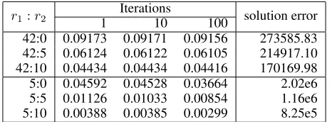
Experiments with the Optimistic Search Algorithm. We do experiments with the Optimistic Search Algorithm, as discussed in Section 4.3. The results are shown in Table 4. Observe that the solution error does not change, but the rel-ative error bound is being reduced (slightly) with additional iterations.

7 Concluding remarks

(8)

r1:r2 ₁ Iterations₁₀ ₁₀₀ solution error

42:0 0.09173 0.09171 0.09156 273585.83 42:5 0.06124 0.06122 0.06105 214917.10 42:10 0.04434 0.04434 0.04416 170169.98 5:0 0.04592 0.04528 0.03664 2.02e6 5:5 0.01126 0.01033 0.00854 1.16e6 5:10 0.00388 0.00385 0.00299 8.25e5

Table 4: Relativea posteriori bounds of the Greedy HLR with Optimistic Search Algorithm on the TechTC01 dataset

An algorithm that uses the “best-first” heuristic search ap-proach was described. Three variants, optimal, suboptimal and greedy, were described, This heuristic search technique allows us to computea priorianda posterioribounds, which show how close the results are to the optimal solution.A pri-oribounds can be computed before the run of the algorithm.

A posterioribounds can be computed after termination. The paper also shows how to use thea posterioribound to im-prove the solution accuracy.

A short abstract describing some of the results in this pa-per appears in (Shah et al. 2018b). Similar ideas were also used to derive new algorithms for robust PCA. See (Shah et al. 2017; 2018a).

References

Arai, H.; Maung, C.; Xu, K.; and Schweitzer, H. 2016. Unsuper-vised feature selection by heuristic search with provable bounds on suboptimality. InAAAI’16, 666–672.

Arai, H.; Maung, C.; and Schweitzer, H. 2015. Optimal column subset selection by A-Star search. InAAAI’15, 1079–1085. Boutsidis, C.; Mahoney, M. W.; and Drineas, P. 2009. An improved approximation algorithm for the column subset selection problem. InSODA, 968–977.

Bringmann, K.; Kolev, P.; and Woodruff, D. P. 2017. Approxima-tion algorithms for`0-low rank approximation. InNIPS’17. Curran Associates, Inc.

Businger, P., and Golub, G. H. 1965. Linear least squares solutions by Householder transformations.Numer. Math.7:269–276. Chierichetti, F.; Gollapudi, S.; Kumar, R.; Lattanzi, S.; Panigrahy, R.; and Woodruff, D. P. 2017. Algorithms for`plow-rank approx-imation. InProceedings of the 34th International Conference on Machine Learning, volume 70, 806–814. PMLR.

Deshpande, A., and Rademacher, L. 2010. Efficient volume sam-pling for row/column subset selection. InFOCS, 329–338. IEEE Computer Society Press.

Deshpande, A.; Rademacher, L.; Vempala, S.; and Wang, G. 2006. Matrix approximation and projective clustering via volume sam-pling.Theory of Computing2(12):225–247.

Drineas, P.; Mahoney, M.; and Muthukrishnan, S. 2008. Relative-error CUR matrix decompositions.SIAM Journal on Matrix Anal-ysis and Applications30(2):844–881.

Gillis, N., and Vavasis, S. A. 2018. On the complexity of robust pca and l1-norm low-rank matrix approximation. Mathematics of Operations Researchin press.

Golub, G. H., and Van-Loan, C. F. 2013. Matrix Computations. Johns Hopkins University Press, fourth edition.

Gu, M., and Eisenstat, S. C. 1996. Efficient algorithms for comput-ing a strong rank-revealcomput-ing QR factorization. SIAM J. Computing 17(4):848–869.

Guruswami, V., and Sinop, A. K. 2012. Optimal column-based low-rank matrix reconstruction. In Rabani, Y., ed.,Proceedings of the Twenty-Third Annual ACM-SIAM Symposium on Discrete Al-gorithms, SODA 2012, Kyoto, Japan, January 17-19, 2012, 1207– 1214. SIAM.

Guyon, I., and Elisseeff, A. 2003. An introduction to variable and feature selection. Journal of Machine Learning Research3:1157– 1182.

Halko, N.; Martinsson, P. G.; and Tropp, J. A. 2011. Finding struc-ture with randomness: Probabilistic algorithms for constructing ap-proximate matrix decompositions.SIAM Review53(2):217–288. Jolliffe, I. T. 2002. Principal Component Analysis. Springer-Verlag, second edition.

Kneip, A., and Sarda, P. 2011. Factor models and variable selection in high-dimensional regression analysis. The Annals of Statistics 39(5):2410–2447.

Li, H.; Linderman, G. C.; Szlam, A.; Stanton, K. P.; Kluger, Y.; and Tygert, M. 2017. Algorithm 971: An implementation of a random-ized algorithm for principal component analysis.ACM Trans Math Softw.43(3):28:1–28:14.

Maung, C., and Schweitzer, H. 2013. Pass-efficient unsupervised feature selection. InAdvances in Neural Information Processing Systems (NIPS), volume 26, 1628–1636.

Paul, S.; Magdon-Ismail, M.; and Drineas, P. 2015. Column se-lection via adaptive sampling. InNIPS’15. Curran Associates, Inc. 406–414.

Pearl, J. 1984. Heuristics : intelligent search strategies for com-puter. Reading, Massachusetts: Addison-Wesley.

Shah, S.; He, B.; Maung, C.; and Schweitzer, H. 2017. Computing robust principal components by A* search. InIEEE 29th Inter-national Conference on Tools with Artificial Intelligence (ICTAI), 1042 – 1049.

Shah, S.; He, B.; Maung, C.; and Schweitzer, H. 2018a. Computing robust principal components by A* search. International Journal on Artificial Intelligence Tools27(7).

Shah, S.; He, B.; Xu, K.; Maung, C.; and Schweitzer, H. 2018b. Solving generalized column subset selection with heuristic search. InProceedings of the 32nd National Conference on Artificial Intel-ligence (AAAI’18), 8153–8154. AAAI Press.

Shitov, Y. 2017. Column subset selection is np-complete. arXiv e-print (arXiv:1701.02764[math.CO]).

Song, Z.; Woodruff, D. P.; and Zhong, P. 2017. Low rank approxi-mation with entrywise`1-norm error. InSTOC’17, 688–701. New York, NY, USA: ACM.

Thayer, J. T., and Ruml, W. 2008. Faster than weighted a*: An op-timistic approach to bounded suboptimal search. InProceedings of the Eighteenth International Conference on International Confer-ence on Automated Planning and Scheduling, ICAPS’08, 355–362. AAAI Press.

Wang, H. 2012. Factor profiled sure independence screening. Biometrika99(1):15–28.