The Thirty-Third AAAI Conference on Artificial Intelligence (AAAI-19)
SNR: Sub-Network Routing for
Flexible Parameter Sharing in Multi-Task Learning
Jiaqi Ma,
1∗Zhe Zhao,
2Jilin Chen,
2Ang Li,
3Lichan Hong,
2Ed H. Chi
21School of Information, University of Michigan, Ann Arbor 2Google AI 3DeepMind
1[email protected] 2,3{zhezhao, jilinc, anglili, lichan, edchi}@google.com
Abstract
Machine learning applications, such as object detection and content recommendation, often require training a single model to predict multiple targets at the same time. Multi-task learning through neural networks became popular recently, because it not only helps improve the accuracy of many pre-diction tasks when they are related, but also saves computa-tion cost by sharing model architectures and low-level repre-sentations. The latter is critical for real-time large-scale ma-chine learning systems.
However, classic multi-task neural networks may degenerate significantly in accuracy when tasks are less related. Previ-ous works (Misra et al. 2016; Yang and Hospedales 2016; Ma et al. 2018) showed that having more flexible architec-tures in multi-task models, either manually-tuned or soft-parameter-sharing structures like gating networks, helps im-prove the prediction accuracy. However, manual tuning is not scalable, and the previous soft-parameter sharing models are either not flexible enough or computationally expensive. In this work, we propose a novel framework called Sub-Network Routing (SNR) to achieve more flexible parameter sharing while maintaining the computational advantage of the classic multi-task neural-network model. SNR modularizes the shared low-level hidden layers into multiple layers of sub-networks, and controls the connection of sub-networks with learnable latent variables to achieve flexible parameter shar-ing. We demonstrate the effectiveness of our approach on a large-scale dataset YouTube8M. We show that the proposed method improves the accuracy of multi-task models while maintaining their computation efficiency.
Introduction
In recent years, neural network based multi-task learning (Caruna 1993; Caruana 1998) has been successfully applied to a variety of real-world applications such as real-time ob-ject detection (Girshick 2015; Ren et al. 2015) and online recommender systems (Bansal, Belanger, and McCallum 2016; Ma et al. 2018). Given a single input, these systems usually predict multiple targets (or categories) at the same time. They often have low-latency requirement at the serving time. For example, a movie recommender system may need to predict both the probability of a user clicking a movie
∗
Work done while interning at Google.
Copyright c⃝2019, Association for the Advancement of Artificial Intelligence (www.aaai.org). All rights reserved.
and that of a user liking watching a movie, so as to decide whether or not to recommend the movie in milliseconds. The many concurrent tasks, the low latency requirement, and the large exploration space of user and movie combination make efficient multi-task learning highly desirable.
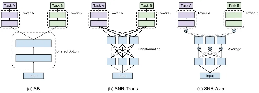
Figure 1(a) provides an illustration of a classic yet widely-used multi-task learning model (Caruana 1998), which we call Shared-Bottom (SB) model. This model consists of sev-eral large low-level layers (Shared-Bottom) that are shared by all tasks, and several small task-specific high-level lay-ers built on top of the shared laylay-ers. Compared to having a separate model for each task, the SB model learns a joint representation of many related tasks which can not only im-prove its model accuracy, but also save computation cost at serving time by sharing low-level network layers.
Despite many successful use cases in multi-task learn-ing, the classic SB model is known to suffer from signifi-cant degeneration in accuracy when tasks are unrelated to each other (Ma et al. 2018). Compared to single-task mod-els, the SB model introduces inductive bias into the shared low-level layers. When tasks are unrelated, the inductive biases in different tasks will have conflicts and hurt the model accuracy. A straightforward solution to this prob-lem is to try multi-task models as well as single-task
mod-els, i.e., use multi-task models for related tasks and use
single-task models for unrelated tasks. Another solution is to manually tune the network architecture to allow
flexi-ble parameter sharing, i.e., sharing more layers for highly
related tasks and less layers for less related ones. Indeed, Misra et al. (2016) showed that different multi-task archi-tectures are required to work well for two different related pairs of tasks. Note that both solutions rely on the knowl-edge of task relatedness. Despite the effort of several prior works (Baxter 2000; Ben-David, Gehrke, and Schuller 2002; Ben-David and Schuller 2003), efficiently measuring task relatedness in real-world data still remains an open problem. So, for both aforementioned solutions, we need to manually tune model structures by training and optimizing directly on the task accuracies. This usually does not scale for large-scale multi-task problems.
(a) SB
Tower A
Task B
Input Task A
Tower B Tower A
Task B
Input Task A
Tower B Tower A
Task B
Input Task A
Tower B
Shared Bottom
(b) SNR-Trans (c) SNR-Aver
Transformation Average
Figure 1: Multi-task Models. (a) Shared-Bottom (SB) model: the conventional multi-task neural network model. (b) Sub-Network Routing with Transformation (SNR-Trans) model: the shared layers are split into sub-networks and the connection (dashed line) between the sub-networks is a transformation matrix multiplied by a scalar latent variable. (c) Sub-Network Routing with Average (SNR-Aver) model: the shared layers are split into sub-networks and the connection (dashed line) between the sub-networks is a weighted average with scalar latent variables as weights.
al. 2016; Yang and Hospedales 2016; Ma et al. 2018). How-ever, prior approaches often are either of limited flexibility, or flexible but computationally expensive due to incorporat-ing too many substructures. For example, on the limited flex-ibility side, Ma et al. (2018) split the shared layers into one layer of sub-networks, and allowed only limited combina-tions of sharing structures. On the other hand, on the flexi-ble but expensive side, Misra et al. (2016) built a multi-task model by connecting internal layers of single-task models, making the model as costly as multiple single-task models; Yang and Hospedales (2016) used a computationally expen-sive tensor factorization technique.
We propose a novel framework called Sub-Network Rout-ing (SNR) to achieve more flexible parameter sharRout-ing while maintaining the computational advantage of the SB model. SNR framework modularizes the shared low-level layers into parallel sub-networks and learns their connections. Modularization with sub-networks is known to improve the trainability of multi-task models (Ma et al. 2018). The con-nectivity between two sub-networks is controlled by a bi-nary variable, which we call a coding variable. With sev-eral layers of sub-networks and different coding variables, we can model a large set of sharing architectures in multi-task models. The computational advantage of the SB model is also maintained because, the related tasks can utilize the same networks. Depending on how we connect sub-networks, we designed two types of connections in the SNR framework, namely SNR-Trans and SNR-Aver. SNR-Trans (shown in Figure 1(b)) uses matrix transformations to trans-form embeddings from lower-level sub-networks to higher-level sub-network; SNR-Aver (shown in Figure 1(c)) takes a weighted average of embeddings from lower-level sub-networks to high-level sub-sub-networks. Our framework is also related to the area of Neural Architecture Search (NAS) (Zoph and Le 2016) in the sense we are searching for a neu-ral architecture that works best for our tasks at hand. Our
purpose of architecture search is for flexible parameter shing in multi-task learnshing. Therefore we can encode the ar-chitecture space simply by the coding variables in the afore-mentioned SNR frameworks. With modularization, we also have a tradeoff between the flexibility of architecture space and the difficulty of architecture search.
The next question is how to efficiently learn the connec-tions between sub-networks. We model the coding variables as latent random variables from parameterized distributions. The distribution parameters can be trained by gradient-based optimization together with the multi-task model pa-rameters using the reparameterization trick (Kingma and Welling 2013; Rezende, Mohamed, and Wierstra 2014; Louizos, Welling, and Kingma 2017). At serving time, we use a deterministic estimator derived from the learned dis-tribution to get the serving coding variables. This method shares insights with recent works (Pham et al. 2018; Liu, Si-monyan, and Yang 2018) of accelerating NAS, where they showed that reusing model parameters across different net-work architecture samples, and joint learning architectures and model parameters can significantly speed up the process of NAS. The latent variable method also provides additional benefits with sparsity priors or penalties. We incorporate a technique of L0 regularization for neural networks (Louizos, Welling, and Kingma 2017) to further improve the accuracy of SNR-Trans under limited serving model size.
We evaluate our method on a large public video dataset, YouTube8M (Abu-El-Haija et al. 2016). This dataset
con-sists of6.1million of YouTube video IDs, each with
(mul-tiple) labels from a vocabulary of more than3,000entities.
The input features of each video ID are pre-computed vi-sual and audio features from the corresponding video. The
3,000+ label classes are organized into 24 top categories.
SNR-Aver significantly outperform several baseline multi-task models. With L0-regularization, we further reduce the serving model size of SNR-Trans by up to 11%.
The rest of this paper is organized as follows: Section 2 reviews related work. Section 3 introduces the proposed ap-proach in details. Section 4 evaluates the proposed models on YouTube8M dataset. Finally, Section 5 concludes the pa-per.
Related Work
Flexible Parameter Sharing in Multi-task Learning
Several related works have been proposed to improve multi-task learning when multi-tasks are less related. Duong et al. (2015) split the multi-task model into two single-task models and added an L2 constraint between the difference of their model parameters. The Cross-Stitch model (Misra et al. 2016) also split the multi-task model into single-task mod-els and concatenated the low-level layers of different single-task models weighted by learnable parameters. Yang and Hospedales (2016) used a tensor factorization model to gen-erate hidden-layer parameters for each task. All of the above methods are not designed to maintain the computational ad-vantage in the classic SB model. The model in Duong et al. (2015) is specifically designed for two-task scenario and cannot directly generalize to many-task scenario.The closest work along this line is the MMoE model Ma et al. (2018), which split the shared low-level layers into sub-networks (called experts) and used different gating net-works for different tasks to utilize different sub-netnet-works. Our approach generalizes this idea into a more flexible form. Our approach also allows sparse connections among sub-networks, which further improves the serving computational efficiency.
Neural Architecture Search
Neural Architecture Search (NAS) (Zoph and Le 2016; Zoph et al. 2017; Real et al. 2018; Pham et al. 2018; Liu, Simonyan, and Yang 2018) is an emerging area of meth-ods that automatically design neural architectures for a given task by reinforcement learning or evolution strategy. Our ap-proach searches for a multi-task model architecture that can both alleviate the task conflicts and maintain the computa-tion efficiency at serving time, which can be viewed as a special case of NAS. We specifically care about the param-eter sharing problem and have a simpler architecture space within the proposed SNR framework.
The very first NAS method (Zoph and Le 2016) used a double-loop approach to search model architectures: in the outer-loop, an RNN-based controller generates model ar-chitectures and is trained with reinforcement learning re-warded by the accuracy of the generated architectures; in the inner-loop, the generated architecture is trained on the target task. As can be imagined, this process is very compu-tational expensive. Several recent works (Pham et al. 2018; Liu, Simonyan, and Yang 2018) have been proposed for ef-ficient NAS by merging the double-loop process and learn-ing the architecture and model parameters simultaneously. Our approach shares similar insights with these efficient
NAS methods in the sense that we learn the architecture and model parameters together. However, as we have a relatively simpler architecture space, we can treat the coding variables as latent random variables and use a simple parametrized distribution (a continuous relaxation of Bernoulli distribu-tion) as the policy to generate the architectures, which is more efficient to train.
Approach
In this section, we introduce the proposed approach in de-tails.
Sub-Network Modularization and Routing
We aim to improve multi-task learning models by flexi-ble parameter sharing, where we want to make more re-lated tasks share more model parameters and less rere-lated tasks share fewer model parameters. Several previous works (Misra et al. 2016; Ma et al. 2018) approached this goal by splitting the whole neural network model into some forms of sub-networks, allowing different tasks to utilize different sub-networks. Ma et al. (2018) showed that such modular-ization benefits the trainability of multi-task models. In this work, we further extend this idea by modularizing each of the shared low-level layers in the classic SB model into par-allel sub-networks (see Figure 1 (b) and (c)).
Based on such modularization, we can have different ex-tents of parameter sharing in the multi-task model by con-trolling the connection routing among the sub-networks of different layers. We call this framework Sub-Network Rout-ing (SNR). By explorRout-ing a large set of connection patterns, we hope to find a good architecture that shares the sub-networks as much as possible so that it can both alleviate the task conflicts and maintain the computation efficiency at serving time.
There are many choices of the routing between sub-networks. We implement two natural types: the first type, which we call SNR-Trans (shown in Figure 1(b)), is to use a transformation matrix multiplied by a scalar coding vari-able; the second type, which we call SNR-Aver (shown in Figure 1(c)), is to have a weighted average with scalar cod-ing variables as weights.
Suppose there are two subsequent layers of sub-networks, and the lower-level layer has 3 sub-networks and the
higher-level layer has 2 sub-networks. Letuuu111, uuu222, uuu333be the outputs
of the lower-level sub-networks and letvvv111, vvv222be the inputs
of the higher-level sub-networks. Then SNR-Trans can be formulated as
[ v1 v1 v1 v2 v2 v2 ]
=
[
z11WWW111111 z12WWW121212 z13WWW131313 z21WWW212121 z22WWW222222 z23WWW232323
][uuu111 uuu222 uuu333 ]
whereWijWWijij is a transformation matrix from the jth
lower-level sub-network to theith higher-level sub-network andzzz
represents the coding variables (a group of binary variables controlling the connection).
Similarly, SNR-Aver can be formulated as [
v1 vv11 v2 vv22 ]
=
[
z11III111111 z12III121212 z13III131313 z21III212121 z22III222222 z23III232323
whereIijIIijij is an identity matrix for alli, j.
If we hold the two models having the same number of model parameters (and thus similar model size), SNR-Trans has more model parameters in the connection while SNR-Aver has more budget of model parameters in the sub-networks. Although it is hard to tell the pros and cons in terms of model representation for the two routing schemes, we argue that when applying sparse connections among the sub-networks, it is easier to reduce the model parameters in SNR-Trans than in SNR-Aver, which could benefit model serving.
Connecting to Manual Tuning and NAS
Manually tuning the network architecture is equivalent to
manually setting the coding variableszzz, wherezij∈ {0,1}.
For example, let’s supposevvv111, vvv222 represent the outputs of
sub-networks to two tasks and there is only one layer of
hid-den sub-networksuuu111, uuu222, uuu333. If we set all elements ofzzzas
1, then the corresponding model degenerates to the classic
shared-bottom model. If we setz11=z22= 1and all other
elements ofzzzas0, then the model degenerates to two small
single-task models.
If we have infinite computation resource, manual tun-ing perhaps allows us to find the best architectures that are pareto optimal in terms of prediction accuracy and com-putation efficiency. However, when there are many tasks and many hidden-layers in a multi-task model, the search
space for coding variablezzz becomes exponentially large:
2|zzz|, where|zzz| denotes the number of elements inzzz. As a
result, manual tuning could be very inefficient when we lack the knowledge of task relatedness.
Inspired by the efficient NAS methods mentioned in the related work, we turn to automatically learn the connection routing within the fairly flexible SNR framework. In our sce-nario, our goal is to efficiently explore different multi-task architectures to achieve flexible parameter sharing across tasks rather than general neural architecture search. And we
have a relative constrained architecture space encoded byzzz.
We propose to model the coding variableszzz as latent
ran-dom variables from parameterized distributions, and learn the distribution parameters and model parameters simulta-neously.
Learning the Architecture with Latent Variables
In this section, we formulate the problem of learning the connection routing in the SNR framework with latent vari-ables.Let f(·;WWW , zzz) be a neural network model
parameter-ized by weightsWWW and coding variableszzzwhere the
cod-ing variables is supposed to be drawn from a latent
pol-icy distributionp(zzz;πππ)parametrized byπππ. Given a dataset
D={(xxxi, yyyi)}N
i=1, wherexxxiis a feature vector of the
sam-pleiandyyyiis the corresponding label vector containing the
labels of multiple tasks, the problem of learning coding vari-ables and model parameters can be formulated as an opti-mization problem as follows:
min W W
W ,πππEEEzzz∼p(zzz;πππ) 1 N
N ∑
i=1
L(f(xxxi;W , zzzWW ), yyyi), (1)
whereLis a loss function.
We simply use Bernoulli distributions as our policy for
the coding variableszzz. That iszi ∼ Bern(πi)for all
ele-mentszi inzzz. The coding variables can also be viewed as
latent variables in a graphical model perspective. This la-tent variable method can be applied to both SNR-Trans and SNR-Aver.
The objective function in Eq. 1 is non-differentiablew.r.t.
the distribution parametersπππ, but the gradients can be
esti-mated by gradient estimator REINFORCE (Williams 1992). Louizos, Welling, and Kingma (2017) further proposed a re-laxation to smooth such objective functions so that we can directly calculate the gradients of the distribution parame-ters. We adopt this relaxation method in our model.
The main idea of the method in (Louizos, Welling, and Kingma 2017) is to first find a continuous random variable
s ∼ q(s;φ)and compute the coding variablez as a
hard-sigmoid ofs,i.e.,
z=g(s) = min(1,max(0, s)).
Then, Eq. 1 becomes
min
WWW ,πππEEEsss∼q(sss;φφφ) 1 N
N ∑
i=1
L(f(xxxi;WWW , g(sss)), yyyi). (2)
The objective function 2 is reformulated using the reparam-eterization trick (Kingma and Welling 2013; Rezende, Mo-hamed, and Wierstra 2014; Louizos, Welling, and Kingma 2017) as
min W
WW ,πππEEEϵϵϵ∼r(ϵϵϵ) 1 N
N ∑
i=1
L(f(xxxi;WWW , g(h(φφφ, ϵϵϵ))), yyyi), (3)
whereϵϵϵis a noise random variable,r(ϵϵϵ)is a parameter-free
noise distribution, andh(·,·)is a deterministic and
differen-tiable transformation ofφφφandϵϵϵ.
In practice, the hard concrete distribution (Louizos, Welling, and Kingma 2017) is used, which is defined (element-wise) as follows,
u∼U(0,1), s=sigmoid((log(u)−log(1−u) + log(α)/β)
¯
s=s(ζ−γ) +γ, z= min(1,max(¯s,0)),
whereuis a uniform random variable,log(α)is a learnable
distribution parameter, andβ, γ, ζare all hyper-parameters.
More details about the hard concrete distribution can be found at (Louizos, Welling, and Kingma 2017).
Applying L0 Regularization on Latent Variables
Another benefit of this latent variable model is that we can add priors and regularizations on the latent variables. For example, Louizos, Welling, and Kingma (2017) provided a way to learn sparse latent variables through L0 regulariza-tion. The sparsity structure is also desirable in our scenario because this allows the multi-task model to be computation-ally efficient.The L0 regularization on the latent variableszzzcan be
for-mulated as
EEEzzz∼p(zzz;πππ)||zzz||0=
|zzz| ∑
i=1
With the relaxation fromzzzto continuous random variables
sss, we have
p(zi= 1;πi) = 1−Q(si<0;φi),
whereQ(·;φi)is the cumulative distribution function ofsi.
So the L0 regularization becomes
E
EEzzz∼p(zzz;πππ)||zzz||0=
|zzz| ∑
i=1
1−Q(si<0;φi).
The full objective function with L0 regularization is
E E Eϵϵϵ∼r(ϵϵϵ)
1 N
N ∑
i=1
L(f(xxxi;WWW , g(h(φφφ, ϵϵϵ))), yyyi)
+λ |zzz| ∑
j=1
1−Q(sj<0;φj),
whereλis a hyper-parameter (see the Experiment Setup
sec-tion for more details).
Additional Details of Model Training and Serving
The whole model, including both model parametersWWW and
latent variable distribution parameterslog(ααα), is trained by
stochastic gradient based optimization. For each mini-batch in the forward pass, we first sample a group of uniform
ran-dom variablesuuu, then calculatezzzto obtain the network
ar-chitecture, and finally feed the input data into the model to
compute the loss. The gradientsw.r.t.WWWandlog(ααα)are
cal-culated by back-propagation. Multiple samples ofuuucan be
drawn to reduce the variance of the gradient estimates but
one sample ofuuuper mini-batch works well in practice.
At serving time, the following estimator (Louizos,
Welling, and Kingma 2017) is used forzzz,
ˆ
zzz= min(1,max(0,sigmoid(log(ααα))(ζ−γ) +γ)).
When sigmoid(log(αij))(ζ −γ) +γ < 0, we will have
ˆ
zij = 0and the resulted model will be sparsely connected.
To reduce serving model parameter size in SNR-Aver model, we need to remove at least a whole sub-network from
the model, which means we need to havezˆij = 0for alli
to eliminate thejth sub-network. For SNR-Trans, however,
anyzijˆ = 0will eliminate the correspondingWij from the
model. So it’s easier to reduce model parameters in SNR-Trans than in SNR-Aver.
Experiment
In this section, we conduct experiments on a public large-scale dataset, YouTube8M, to evaluate the effectiveness of the proposed models.
Experimental Setup
YouTube8M Dataset
We use YouTube8M (Abu-El-Haija et al. 2016) as our benchmark dataset to evaluate the effectiveness of the pro-posed methods. This dataset consists of 6.1 million of
SB MMoE ML-MMoE SNR-Aver SNR-Trans Model
0.81 0.82 0.83 0.84 0.85 0.86
Macro Average-MAP@10
Performance on Macro Average-MAP@10
(a) Macro Average-MAP@10
SB MMoE ML-MMoE SNR-Aver SNR-Trans Model
0.81 0.82 0.83 0.84 0.85 0.86
Micro Average-MAP@10
Performance on Micro Average-MAP@10
(b) Micro Average-MAP@10
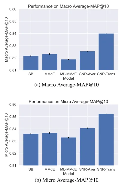
Figure 2: Accuracy of Best-Tuned Models. The bar chart shows the average test performance of the top 10 models selected by validation performance. The error bar indicates the standard error of the average test performance.
YouTube videos, each with (multiple) labels from a
vocabu-lary of more than3,000topical entities. The topical entities
can be further grouped into 24 top-level topic categories. To create a multi-task learning problem from the dataset, we treat each top-level topic category as a separate predic-tion task, so that each task is a multi-label classificapredic-tion problem. To ensure data quantity per task, we used the top 16 categories in data volume.
We use the training set provided in the original dataset as our training set, and split the original validation set into our own validation set and test set, because this dataset comes from a Kaggle competition and the original test set labels are hidden to the public.
Methods
We compare five multi-task learning models in the ex-periments. As the main difference among the models lies in their shared low-level part, we fix the task-specific high-level part of all models as a one-layer fully-connected hid-den layer with hidhid-den size 16 for each task. ReLU activa-tion is used whenever applicable. The implementaactiva-tion of the shared low-level part for each model is described as follows respectively,
several low-level network layers are shared by all the tasks and each task has its own task-specific high-level layers built on top of the shared layers.
Shared part: Two fully-connected hidden layers with the hidden layer sizes as hyper-parameters to be tuned.
MMoE (Ma et al. 2018): This model splits the shared
low-level layers into sub-networks and uses different gating net-works for different tasks to utilize different sub-netnet-works.
Shared part: One fully-connected hidden layer followed by a MMoE layer with 8 experts, each expert being a one-layer fully-connected sub-network. Both the hidden size of the first hidden layer and that of the sub-network are hyper-parameters to be tuned. The gating networks are linear trans-formations without hyper-parameters.
ML-MMoE: This model extends MMoE by adding multi-ple layers of sub-networks. The connections from the lower-level sub-networks to the higher-lower-level sub-networks are also controlled by some gating networks. Each higher-level sub-network can be viewed as an internal task. All the gating net-works share the same input, which is the input of the whole model.
Shared part: Two subsequent MMoE layers with each layer having 8 experts. Each expert is a one-layer fully-connected sub-network. The hidden size of the expert net-work is a tunable hyper-parameter.
SNR-Trans : This is the proposed Sub-Network Routing with Transformation model.
Shared part: Two subsequent transformation layers. The output size of each transformation matrix is tunable.
SNR-Aver: This is the proposed Sub-Network Routing with Averaging model.
Shared part: Two subsequent sub-network layers with each sub-network being a one-layer fully-connected net-work. The hidden size of each sub-network is tunable.
Evaluation Metrics
As each task in the YouTube8M dataset is a multi-label classification problem, we use Mean Average Precision (MAP) as the measurement of prediction accuracy for each task. Specifically, we use MAP@10 as our metric because most of the examples have fewer than 10 positive labels in each task. To evaluate the overall accuracy of the multi-task models, we compute an average of the MAP@10 of all tasks, which we will call it Average-MAP@10. As differ-ent tasks have differdiffer-ent sample sizes, we calculate two types of Average-MAP@10 metrics: the first type directly calcu-lates the mean of the MAP@10 scores of all the tasks, which we call Macro Average-MAP@10; the second type takes a weighted average of the MAP@10 scores weighted by the number of data examples in each task, which we call Micro Average-MAP@10.
Model Training and Hyper-parameter Tuning
All the models are trained using Adam (Kingma and Welling 2013) with learning rate as a tunable
hyper-parameter. The batch size is fixed as 128. Early stopping
is used on the validation set. Model size related
hyper-3 × 10
64 × 10
66 × 10
6# Model Parameters (Log-Scale)
0.815 0.820 0.825 0.830 0.835 0.840
Macro Average-MAP@10
Macro Average-MAP@10 vs # Model Parameters
SNR-Trans SNR-Aver SB MMoE
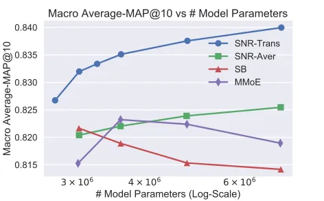
Figure 3: Macro Average-MAP@10 vs Model Size. The y-axis is the test performance on Macro Average-MAP@10. The x-axis is the number of total model parameters at train-ing time. The total hidden size of first shared layer in each model is fixed as 2048 and the total hidden size of the second shared layer is varied to get different model sizes.
parameters are tuned with grid search for the purpose of comparing model accuracy at different model size, and all other hyper-parameters are tuned with random search. The hidden sizes of the two shared hidden layers in SB are
grid-searched from {256,512,1024,2048} and the hidden
size hyper-parameters in other models are grid-searched in a way to approximately match the model size of SB.
The L0 regularization parameter λ will have an impact
on the serving model size so we grid-search it from {0.001,0.0001,0.00001}. The learning rates of all
mod-els are random-searched within[0.00001,0.1]in log-scale.
The hyper-parameters for the hard concrete distribution used in L-Act and L-Param models are random-searched from
the following range: β ∼ [0.5,0.9], γ ∼ [−1,−0.1], ζ ∼
[1.1,2].
For each model size setting, we run 500 independent trials of random search on hyper-parameters unrelated to model size and select the top 10 models with best validation accu-racy. Then we report the average and the standard error of testing MAPs from these top 10 models.
Results
Accuracy of Best-Tuned Models
We first show the accuracy of the best-tuned models using each method in Figure 2. We report the test accuracy on both Macro Average-MAP@10 and Micro Average-MAP@10. The differences between each pair of models on both met-rics, except for MMoE vs SB on Micro Average-MAP@10, are significant with 0.05 significance level of two-sample t-test. The relative trends on both metrics are the same. So we will show the results of Macro Average-MAP@10 only in the remaining result analysis due to page limit.
11% Less
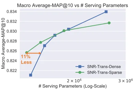
Figure 4: Macro Average-MAP@10 of SNR-Trans models with different model sizes and L0 regularization parameters. “SNR-Trans-Dense” indicates models that use a small L0 regularization parameter and the resulted models are dense; “SNR-Trans-Sparse” indicates models that use a large L0 regularization parameter and the resulted models are sparse. The sparse models can reduce the serving model size by up to 11% under certain serving constraint.
Arts_Entertainment
Games
Autos_Vehicles
Sports
Food_Drink
Computers_Electronics
Business_Industrial
Pets_Animals
Hobbies_Leisure Beauty_Fitness
Shopping
Internet_Telecom Home_Garden Science Travel
Law_Government
0.00 0.02 0.04 0.06 0.08 0.10
Relative Proportion of Utilization
Sub-Network Utilization by Tasks
Figure 5: Average sub-network utilization by tasks in top performing SNR-Trans models. The tasks on x-axis are sorted by sample size in descending order from left to right. The y-axis is the average relative proportion of sub-networks utilized by the corresponding task.
may cause difficulty in optimization. There is also a design difficulty of selecting the input layer of gating networks that lie between two layers of experts. As there are many inter-nal outputs from the previous layer of experts, it is hard to decide which internal outputs should be used by the higher-level gating networks. In our implementation, we use the ini-tial input features of the first layer as the input of all gating networks. However, the initial input features may not
pro-vide enough information about how to route in higher-level layers.
Accuracy vs Model Size
One thing which we notice during the hyper-parameter tuning is that, while the accuracy of baseline models has sat-urated as we increase the model size, the accuracy of SNR-Trans and SNR-Aver still slowly increases at the boundary of our hyper-parameter range.
Figure 3 shows the test accuracy of a sampled set of mod-els with different model sizes. In this figure, we fix the total
hidden size of the first shared layer in each model as2048,
and we vary the total hidden size of the second shared layer to get models with different model sizes. Note that the x-axis is the number of total model parameters at training time, which means the model parameters eliminated by L0 regu-larization in SNR models are also counted.
This result shows that the SNR method can train larger models better than baseline methods. This phenomenon aligns well with our hypothesis that modularization in multi-task learning could improve model trainability.
Accuracy of Sparse Models
While being able to train large models well is critical, in many large-scale online systems we have strict low-latency requirements on the serving model. So we also care about models with limited serving model sizes. Here we show that
with a proper L0 regularization parameterλ, we can
effec-tively reduce the serving model size of the SNR-Trans model under certain serving constraints.
We first observe that the value of the L0 regularization
parameter λ has a direct impact on the learned
architec-ture of SNR-Trans models. When λis set to 0.00001, the
learned coding variablesz are almost all1s, which means
the learned architecture is densely connected. Whenλis set
to0.0001, the learned architecture is sparse and the sparse
model has significantly smaller serving model size than the dense model. Given the same training model size, the sparse model usually performs worse than the dense model. This
result is not unexpected as λ controls a tradeoff between
higher model capacity and smaller serving model size, with
largeλshrinking the effective capacity for the model.
How-ever, when the serving model size is limited, the sparse model outperforms the dense model that has similar serving model size.
As shown in Figure 4, “SNR-Trans-Dense” indicates SNR-Trans models with L0 regularization parameter
0.00001 while “SNR-Trans-Sparse” indicates SNR-Trans
models with L0 regularization parameter0.0001. We fix the
Analysis of Sub-Network Utilization
To better understand how the sub-networks are utilized by different tasks in the sparse models, we further summa-rize the average relative proportion of sub-networks used by each task in 10 top performing sparse models, shown in Fig-ure 5. The figFig-ure shows that the utilization of sub-networks
is positively related to the sample size of the tasks1. This
im-plies that, when we add a stronger L0 regularization on the model, the model will learn to allocate more capacity to the tasks with more data.
Conclusion
In this work, we introduce a flexible parameter sharing framework in multi-task learning, Sub-Network Routing (SNR). SNR is able to encode various types of multi-task model architectures and allows us to add a wide range of priors on the model structure. We propose a scalable multi-task architecture search solution by using latent variables to model the architecture coding variables, and learning the la-tent variables and model parameters simultaneously. We em-pirically show that the proposed methods outperform base-line multi-task models on a large-scale dataset YouTube8M. We further reduce the serving model size by applying L0 regularization on the latent variables.
References
Abu-El-Haija, S.; Kothari, N.; Lee, J.; Natsev, P.; Toderici,
G.; Varadarajan, B.; and Vijayanarasimhan, S. 2016.
Youtube-8m: A large-scale video classification benchmark. arXiv preprint arXiv:1609.08675.
Bansal, T.; Belanger, D.; and McCallum, A. 2016. Ask the gru: Multi-task learning for deep text recommendations. In Proceedings of the 10th ACM Conference on Recommender Systems, 107–114. ACM.
Baxter, J. 2000. A model of inductive bias learning.Journal
of Artificial Intelligence Research12:149–198.
Ben-David, S., and Schuller, R. 2003. Exploiting task
relat-edness for multiple task learning. InLearning Theory and
Kernel Machines. Springer. 567–580.
Ben-David, S.; Gehrke, J.; and Schuller, R. 2002. A theo-retical framework for learning from a pool of disparate data
sources. InProceedings of the eighth ACM SIGKDD
inter-national conference on Knowledge discovery and data
min-ing, 443–449. ACM.
Caruana, R. 1998. Multitask learning. InLearning to learn.
Springer. 95–133.
Caruna, R. 1993. Multitask learning: A knowledge-based
source of inductive bias. InMachine Learning: Proceedings
of the Tenth International Conference, 41–48.
Duong, L.; Cohn, T.; Bird, S.; and Cook, P. 2015. Low re-source dependency parsing: Cross-lingual parameter sharing
in a neural network parser. InACL (2), 845–850.
Girshick, R. 2015. Fast r-cnn. InProceedings of the IEEE
international conference on computer vision, 1440–1448.
1
The original data distribution of YouTube8M can be found at https://research.google.com/youtube8m/
Kingma, D. P., and Welling, M. 2013. Auto-encoding
vari-ational bayes. arXiv preprint arXiv:1312.6114.
Liu, H.; Simonyan, K.; and Yang, Y. 2018. Darts:
Differen-tiable architecture search.arXiv preprint arXiv:1806.09055.
Louizos, C.; Welling, M.; and Kingma, D. P. 2017.
Learn-ing sparse neural networks throughl 0regularization.arXiv
preprint arXiv:1712.01312.
Ma, J.; Zhao, Z.; Yi, X.; Chen, J.; Hong, L.; and Chi, E. H. 2018. Modeling task relationships in multi-task learning
with multi-gate mixture-of-experts. InProceedings of the
24th ACM SIGKDD International Conference on Knowl-edge Discovery & Data Mining, 1930–1939. ACM. Misra, I.; Shrivastava, A.; Gupta, A.; and Hebert, M. 2016.
Cross-stitch networks for multi-task learning. In
Proceed-ings of the IEEE Conference on Computer Vision and Pat-tern Recognition, 3994–4003.
Pham, H.; Guan, M. Y.; Zoph, B.; Le, Q. V.; and Dean, J. 2018. Efficient neural architecture search via parameter
sharing.arXiv preprint arXiv:1802.03268.
Real, E.; Aggarwal, A.; Huang, Y.; and Le, Q. V. 2018. Reg-ularized evolution for image classifier architecture search. arXiv preprint arXiv:1802.01548.
Ren, S.; He, K.; Girshick, R.; and Sun, J. 2015. Faster r-cnn: Towards real-time object detection with region proposal
net-works. InAdvances in neural information processing
sys-tems, 91–99.
Rezende, D. J.; Mohamed, S.; and Wierstra, D. 2014.
Stochastic backpropagation and approximate inference in
deep generative models. arXiv preprint arXiv:1401.4082.
Williams, R. J. 1992. Simple statistical gradient-following
algorithms for connectionist reinforcement learning.
Ma-chine learning8(3-4):229–256.
Yang, Y., and Hospedales, T. 2016. Deep multi-task
rep-resentation learning: A tensor factorisation approach. arXiv
preprint arXiv:1605.06391.
Zoph, B., and Le, Q. V. 2016. Neural
architec-ture search with reinforcement learning. arXiv preprint
arXiv:1611.01578.
Zoph, B.; Vasudevan, V.; Shlens, J.; and Le, Q. V. 2017. Learning transferable architectures for scalable