The Thirty-Third AAAI Conference on Artificial Intelligence (AAAI-19)
Comparative Document Summarisation via Classification
Umanga Bista,
?‡Alexander Mathews,
?‡Minjeong Shin,
?‡Aditya Krishna Menon,
?∗Lexing Xie
?‡Australian National University?, Data to Decisions CRC‡
{umanga.bista,alex.mathews,minjeong.shin,aditya.menon,lexing.xie}@anu.edu.au
Abstract
This paper considers extractive summarisation in acomparative
setting: given two or more document groups (e.g., separated by publication time), the goal is to select a small number of documents that are representative of each group, and also maximally distinguishable from other groups. We formulate a set of new objective functions for this problem that connect recent literature on document summarisation, interpretable machine learning, and data subset selection. In particular, by casting the problem as a binary classification amongst dif-ferent groups, we derive objectives based on the notion of maximum mean discrepancy, as well as a simple yet effective gradient-based optimisation strategy. Our new formulation allows scalable evaluations of comparative summarisation as a classification task, both automatically and via crowd-sourcing. To this end, we evaluate comparative summarisation methods on a newly curated collection of controversial news topics over 13 months. We observe that gradient-based optimisation outper-forms discrete and baseline approaches in 15 out of 24 different automatic evaluation settings. In crowd-sourced evaluations, summaries from gradient optimisation elicit 7% more accurate classification from human workers than discrete optimisation. Our result contrasts with recent literature on submodular data subset selection that favours discrete optimisation. We posit that our formulation of comparative summarisation will prove useful in a diverse range of use cases such as comparing content sources, authors, related topics, or distinct view points.
1
Introduction
Extractive summarisation is the task of selecting a few repre-sentative documents from a larger collection. In this paper, we
considercomparative summarisation: givengroupsof
docu-ment collections, the aim is to select docudocu-ments that represent
each group, but also highlight differencesbetweengroups.
This is in contrast to traditional document summaries which aim to represent each group by independently optimising for coverage and diversity, without considering other groups. As a concrete example, given thousands of news articles per month on a certain topic, groups can be formed by publication time, by source, or by political leaning. Comparative sum-marisation systems can then help answer user questions such as: what is new on the topic of climate change this week, what
∗
Now at Google Research.
Copyright © 2019, Association for the Advancement of Artificial Intelligence (www.aaai.org). All rights reserved.
time
Feb 2018 Mar 2018
News Media
AAAI Times
ML Daily News
World News
CS Press
Local News
Figure 1: An illustrative example of comparative summarisa-tion. Squares are news articles, rows denote different news
outlets, and thex-axis denotes time. The shaded articles are
chosen to represent AI-related news during Feb and March 2018, respectively. They aim to summarise topics in each
month, and also highlight differencesbetweenthe two months.
is different between the coverage in NYTimes and BBC, or what are the key articles covering the carbon tax and the Paris agreement? In this work, we focus on highlighting changes within a long running news topic over time; see Figure 1 for an illustration.
Existing methods for extractive summarisation use a va-riety of formulations such as structured prediction (Li et al. 2009), optimisation of submodular functions (Lin and Bilmes 2011), dataset interpretability (Kim, Khanna, and Koyejo 2016), and dataset selection via submodular opti-misation (Mirzasoleiman, Badanidiyuru, and Karbasi 2016; Wei, Iyer, and Bilmes 2015; Mitrovic et al. 2018). More-over, recent formulations of comparative summarisation use discriminative sentence selection (Wang et al. 2012; Li, Li, and Li 2012), or highlight differences in common con-cepts across documents (Huang, Wan, and Xiao 2011). But the connections and distinctions of these approaches has yet to be clearly articulated. To evaluate summaries, traditional
approaches employ automatic metrics such asROUGE (Lin
2004) on manually constructed summaries (Lin and Hovy 2003; Nenkova, Passonneau, and McKeown 2007). This is difficult to employ for new tasks and new datasets, and does not scale.
Our approach to comparative summarisation is based on a
novel formulation of the problem in terms of twocompeting
classifier can distinguish them from documents belonging to
othergroups, but cannot distinguish them from documents
belonging to thesamegroup. We show how this framework
encompasses an existing nearest neighbour objective for summarisation, and propose two new objectives based on the
maximum mean discrepancy (Gretton et al. 2012) –mmd-diff
which emphasises classification accuracy andmmd-divwhich
emphasises summary diversity – as well as new gradient-based optimisation strategies for these objectives.
A key advantage of our discriminative problem setting is that it allows summarisation to be evaluated as a classification task. To this end, we design automatic and crowd-sourced evaluations for comparative summaries, which we apply on a new dataset of three ongoing controversial news topics. We observe that the new objectives with gradient optimisation are top-performing in 15 out of 24 settings (across news topics, summary size, and classifiers) (§6.2). We design a new crowd-sourced article classification task for human evaluation. We find that workers are on average 7% more accurate in
classifying articles using summaries generated bymmd-diff
with gradient-based optimisation than all alternatives. Inter-estingly, our results contrast with the body of work on dataset selection and summarisation that favour discrete greedy op-timisation of submodular objectives due to approximation guarantees. We hypothesise that the comparative summari-sation problem is particularly amenable to gradient-based optimisation due to the small number of prototypes needed. Moreover, gradient-based approaches can further improve solutions found by greedy approaches.
In sum, the main contributions of this work are:
• A new formulation of comparative document summari-sation in terms of competing binary classifiers, two new objectives based on this formulation, and their correspond-ing gradient-based optimisation strategies.
• Design of a scalable automatic and human evaluation methodology for comparative summarisation models, with results showing that the new objectives out-perform existing submodular objectives.
• A use case of comparatively summarising articles over time
from a news topic on a new dataset1of three controversial
news topics from 2017 to 2018.
2
Related Works
The broader context of this work is extractive summarisation. Approaches to this problem include incorporating diversity measures from information-retrieval (Carbonell and Goldstein 1998), structured SVM regularised by constraints for diversity, coverage, and balance (Li et al. 2009), or topic models for sum-marisation (Haghighi and Vanderwende 2009). Time-aware summarisation is an emerging subproblem, where the current focus is on modeling continuity (Ren et al. 2016) or contin-uously updating summaries (Rücklé and Gurevych 2017), rather than formulating comparisons. (Li, Li, and Li 2012; Wang et al. 2012) present methods to extract one or few
1Code, datasets and a supplementary appendix are available at https://github.com/computationalmedia/compsumm
discriminative sentences from a small multi-document cor-pus utilising greedy optimisation and evaluating qualitatively. (Huang, Wan, and Xiao 2011) compares descriptions about similar concepts in closely related document pairs, leveraging an integer linear program and evaluating with few manually created ground truth summaries. While these works exist in the domain of comparative summarisation, they are either specific to a data domain or have evaluations which are hard to scale up. In this paper we present approaches to compar-ative summarisation with intuition from competing binary classifiers, leading to different objectives and evaluation. We demonstrate and evaluate the application of these approaches to multiple data domains such as images and text.
Submodular functions have been the preferred form of discrete objectives for summarising text (Lin and Bilmes 2011), images (Simon, Snavely, and Seitz 2007) and data subset selection (Wei, Iyer, and Bilmes 2015; Mitrovic et al. 2018), since they can be optimised greedily with tightly-bounded guarantees. The topic of interpreting dataset and models use similar strategies (Kim, Khanna, and Koyejo 2016; Bien and Tibshirani 2011). This work re-investigates classic continuous optimisation for comparative summarisation, and puts it back on the map as a competitive strategy.
3
Comparative Summarisation as
Classification
Formally, the comparative summarisation problem is defined
onGgroups of document collections{X1, . . . ,XG}, where
a group may, for example, correspond to news articles about a specific topic published in a certain month. We write the
document collection for groupgas
Xg={xg,1,xg,2, . . . ,xg,Ng}
whereNgis the total number of documents in groupg. We
represent individual documents as vectorxg,i∈Rd(see §6).
Our goal is to summarise each document collectionXg
with a set ofsummary documentsorprototypesX¯g ⊂Xg,
written
¯
Xg={¯xg,1,x¯g,2, . . . ,x¯g,M}
For simplicity, we assume the number of prototypesM is
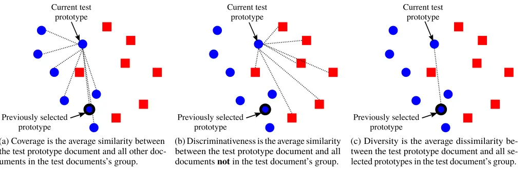
the same for each group. The selected prototypes should represent the documents in the group achieving coverage (Figure 2a) and diversity (Figure 2c), while simultaneously discriminating documents from other groups (Figure 2b). For
example, if we have news articles on theClimate Changetopic
then they may discuss theparis agreementin February,coral
bleachingin March, andrising sea levelsin both months. A
comparative summary should include documents about the
paris agreementin February andcoral bleachingin March,
but potentially not onrising sea levelsas they are common to
both time ranges and hence do not discriminate.
3.1
A Binary Classification Perspective
We now cast comparative summarisation as a binary classifi-cation problem. To do so, let us re-interpret the two defining
Previously selected prototype
Current test prototype
(a) Coverage is the average similarity between the test prototype document and all other doc-uments in the test docdoc-uments’s group.
Previously selected prototype
Current test prototype
(b) Discriminativeness is the average similarity between the test prototype document and all documentsnotin the test document’s group.
Previously selected prototype
Current test prototype
(c) Diversity is the average dissimilarity be-tween the test prototype document and all se-lected prototypes in the test document’s group.
Figure 2: Illustration of coverage, discriminativeness and diversity criteria for selecting prototypes. The two document groups are shown as blue circles and red squares. The dotted lines represent comparisons between pairs of documents.
(i) they must represent the documents belonging to that
group. Intuitively, this means that eachx¯g,i∈X¯gmust
beindistinguishablefrom allxg,j∈Xg.
(ii) they must discriminate against documents from all other
groups. Intuitively, this means that each x¯g,i ∈ X¯g
must bedistinguishablefromx¬g,j∈X¬g, whereX¬g
denotes the set of all documents belonging to all groups
exceptg.
This lets us relate prototype selection to the familiar binary classification problem: for a good set of prototypes,
(a) therecannot exista classifier that can accurately
discrim-inate between them and documents from that group. For example, even a powerful classifier should not be able to discriminate prototype documents about the Great Barrier Reef from other documents about the Great Barrier Reef.
(b) theremust exista classifier that can accurately
discrimi-nate them against documents from all other groups. For example, a reasonable classifier should be able to dis-criminate prototypes about the Great Barrier Reef from documents about emission targets.
Consequently, we can think of prototype selection in terms of two competing binary classification objectives: one
distin-guishingX¯gfromXg, and another distinguishingX¯gfrom
X¬g. In abstract, this suggests a multi-objective optimisation
problem of the form
max
¯
X1,...,X¯G
G
X
g=1
−Acc( ¯Xg,Xg), G
X
g=1
Acc( ¯Xg,X¬g)
!
, (1)
whereAcc(X,Y)estimates the accuracy of the best possible
classifier for distinguishing between the datasetsXandY.
Making this idea practical requires committing to a particular means of balancing the two competing objectives. More interestingly, one also needs to find a tractable way to estimate
Acc(·,·): explicitly searching over rich classifiers such as deep
neural networks, would lead to a computationally challenging nested optimisation problem.
In the following we discuss a set of objective functions that avoid such nested optimisation. We also discuss two simple optimisation strategies for these objectives in §4.
3.2
Prototype Selection via Nearest-neighbour
One existing prototype selection method involves
approxi-mating the intragroupAcc(·,·)term in Eq 1 using
nearest-neighbour classifiers, while ignoring the intergroup accuracy term. Specifically, a formulation of prototype selection in (Wei, Iyer, and Bilmes 2015) maximises the total similarity of every point to its nearest prototype from the same class:
Unn( ¯X) =
G
X
g=1
Ng
X
i=1
max
m∈{1,...,M}Sim(¯xg,m,xg,i) (2)
Here,Simis any similarity function, with admissible choices
including a negative distance, or valid kernel functions. The nearest neighbour utility function is simple and intu-itive. However, it only considers the most similar prototype for each datapoint which misses our second desirable property of prototypes: that they explicitly distinguish between different classes. Moreover, the nearest neighbour utility function can
be challenging to optimise because of themaxfunction. The
rest of this section introduces three other utilities that address these concerns.
3.3
Preliminaries: Maximum Mean Discrepancy
Themaximum mean discrepancy(MMD) (Gretton et al. 2012)
measures the distance between two distributions by leverag-ing the kernel trick (Schölkopf and Smola 2002). Intuitively,
MMD deems two distributions to be close if themeanofevery
function in some rich classFis close under both distributions.
For suitableF, this is equivalent to comparing the moments
of the two distributions; however, a naïve implementation of this idea would require a prohibitive number of evaluations.
Fortunately, choosingFto be a reproducing kernel Hilbert
space (RKHS) with kernel functionk(·,·)leads to an
via the kernel function (Gretton et al. 2012):
MMD2(X,Y) =Ex,x0[k(x,x0)]−2·Ex,y[k(x,y)]+
Ey,y0[k(y,y0)] (3)
wherex ∼X,y ∼Yare observations from two datasets
X,Y. In practice, it is common to use the radial basis function
(RBF) or Gaussian kernelk(x,y) =e−γ·kx−yk2
2with fixed
bandwidthγ >0.
One often approximates MMD using sample
expecta-tions: givennsamplesx1, . . . ,xnfromX, andmsamples
y1, . . . ,ynfromY, we may compute
MMD2(X,Y) = 1 n2
n
X
i=1
n
X
j=1
k(xi,xj)
− 2
mn
n
X
i=1
m
X
j=1
k(xi,yj) +
1 m2
m
X
i=1
m
X
j=1
k(yi,yj) (4)
3.4
Prototype Selection via MMD
One can think of MMD as implicitly computing a (kernelised)
nearest centroid classifier to distinguish between X and
Y: MMD is small when this classifier has high expected
error. Thus, MMD can be seen as an efficient approximation
to classification accuracyAcc(·,·). This intuition lead to a
practical utility function that approximates Equation 1 by taking the difference of two MMD terms:
Udiff( ¯X) =Pg(−MMD 2
( ¯Xg,Xg) +λ·MMD2( ¯Xg,X¬g)) (5)
The hyper-parameter λ trades off how well the
proto-type represents its group, against how well it distinguishes between groups (Figure 2b). Intuitively, when the term
MMD2( ¯Xg,X¬g)is large then the prototypesX¯gare
dissim-ilar from documentsX¬gof other groups. Similarly, when
MMD2( ¯Xg,Xg)is small then the prototypes are similar to
documents of that group. Maximising−MMD2gives
proto-types that are both close to the empirical samples (as seen by
theEx,yterm in Equation 3 and illustrated by Figure 2a) and
far from one another (as seen by theEy,y0term and illustrated
by Figure 2c).
While the objective of Equation 5 provides the core of our approach, we also present a variant that increases the diversity of prototypes chosen for each group. A closer examination
of the difference ofMMD2in Equation 5 – by expanding
both using Equation 3 – reveals two separate prototype
di-versity terms −Ex¯g,x¯0g[k(¯xg,x¯
0
g)] and λE¯xg,x¯0g[k(¯xg,¯x
0
g)]. The latter counteracts the former and decreases prototype
diversity (details in Appendix1). On the expanded form of
λMMD2( ¯Xg,X¬g), we remove the terms not involvingx¯g,
as they are constants and have no effect on the solution, and
also remove the conflicting diversity termλE¯xg,¯x0g[k(¯xg,x¯
0
g)]. This gives a new objective:
Udiv( ¯X) =Pg(−MMD 2( ¯X
g,Xg)−2λEx¯g,x¬g[k(¯xg,x¬g)]) (6)
Maximising −λE¯xg,x¬g[k(¯xg,x¬g)] encourages
proto-types in groupgto be far from data points in other groups.
One can envision another variant that explicitly optimises
the diversity betweenprototypes of different classes, rather
than between prototypes of classgagainst data points in other
classes. This is computationally more efficient, and reflects
similar intuitions. However, it did not outperformUdiff,Udivin
summarisation tasks, and is omitted due to space limitations.
Differences to related objectives. The nearest-neighbour objective was articulated in (Wei, Iyer, and Bilmes 2015) and earlier in (Bien and Tibshirani 2011), and used for classi-fication tasks. Recently, (Kim, Khanna, and Koyejo 2016)
proposedMMD-critic, which selects prototypesX¯ for a single
group of documentsXby maximizing−MMD2( ¯X,X).The
first term in Equation 5 builds on this formulation, applying this idea independently for each group. Our second term
is crucial to encourage prototypes thatonlyrepresent their
own group and none of the other groups.MMD-criticalso
containsmodel criticisms, which have to be optimized
sequen-tially after obtaining prototypes. As shown in §6,MMD-critic
under-performs in comparison tasks by a significant margin.
4
Optimising Utility Functions
There are two general strategies for optimising the utility func-tions outlined in §3 to generate summaries that are a subset of the original dataset: greedy and gradient optimisation.
Greedy optimisation. The first strategy involves directly
choosingM prototypes for each group. Obtaining the exact
solution to this discrete optimisation problem is intractable; however, approximations such as greedy selection can work well in practice, and may also have theoretical guarantees.
Specifically, suppose we wish to maximise a utility set
functionF : 2|V|→
Rdefined on ground setV. ForS⊂V
ands ∈ V \S, the marginal gain of adding elementsto
an existing set S is known as the discrete derivative, and
is defined by∆F(s|S) =F(S∪s)−F(S). We sayF is
monotone if and only if the discrete derivatives are
non-negative, i.e.∆F(s|S)≥0, and is submodular if and only
if the marginal gain satisfies diminishing returns, i.e. for
S⊆T ⊂V, s∈V \T,∆F(s|S)≥∆F(s|T). (Nemhauser,
Wolsey, and Fisher 1978) showed that ifFis submodular and
monotone, greedy maximisation ofFyields an approximate
solution no worse than1−1
e≈0.63of the optimal solution
under cardinality and matroid constraints. (Lin and Bilmes 2010) showed this approximation holds with high probability even for non-monotone submodular objectives.
In our context, given a utility function U, the greedy
algorithm (see Appendix1) works by iteratively picking the
xg that provides the largest marginal gain (∆U(xg|X¯g))
one at a time for each group. Among the utility functions
mentioned in §3, the nearest-neighbour objective Unn is
submodular-monotone (Wei, Iyer, and Bilmes 2015). The MMD function in Equation 3 is submodular-monotone under mild assumptions on the kernel matrix (Kim, Khanna, and
Koyejo 2016). The MMD objective Udiff is the difference
between two submodular-monotone functions, which is not submodular in general. On the other hand, the second term
inUdivis modular with respect toX¯g, when the number of
prototypesM fixed and known in advance. Therefore, the
diversity objectiveUdivis the difference between a submodular
function and a modular function, and thus submodular.
the problem to allow for continuous optimisation in the feature space, e.g. using standard gradient descent. To generate prototypes, the solutions to this optimisation can then be
snappedto the nearest data points as a post-processing step.
Concretely, rather than searching for optimal prototypesX¯g
directly, we seek “meta-prototypes”A¯g={a¯g,1, . . . ,a¯g,M},
drawn from the same space as the document embeddings.
We now modify Udiff (Equation 5) to incorporate
“meta-prototypes”. Note thatUdiv can be similarly modified, but
Unncannot, since themaxfunction is not differentiable. The
“meta-prototypes” forUdiffare chosen to optimise
max
¯ A1,...,A¯G
X
g
(−MMD2( ¯Ag,Xg) +λ·MMD2( ¯Ag,X¬g)) (7)
The only difference to Equation 5 is that we donotenforce
thatA¯g⊂Xg. This subtle, but significant, difference allows
Equation 7 to be optimized using gradient-following methods. We use L-BFGS (Byrd et al. 1995) with analytical gradients
found in online appendix1. The selected meta-prototypesA¯g
are then snapped to the nearest document in the group: to
construct theith prototype for thegth group, we find
¯
xg,i= argmin
xg,j∈Xg
ka¯g,i−xg,jk22. (8)
On a problem often tackled with discrete greedy optimisation, one may wonder if gradient-based methods can be competi-tive; we answer this in the affirmative in our experiments.
5
Datasets on Controversial News Topics
Exploring the evolution of controversial news topics is a nat-ural application of comparative summarisation. Comparative summarisation could help to better understand the role of news media in such a setting. Recent work on controversial topics (Garimella et al. 2018) focused on the social network and interaction around controversial topics, but did not ex-plicitly consider the content of news articles on these topics. To this end, we curate a set of news articles on long-running controversial topics using tweets which link to news articles. We choose several long-running controversial topics with significant news coverage in 2017 and 2018. To find articles relevant to these topics we use keywords to filter the Twitter stream, and adopt a snowball strategy to add additional key-words (Verkamp and Gupta 2013). The articles linked in these tweets are then de-duplicated and filtered for spam. Article timestamps correspond to the creation time of the first tweet linking to it. Full details of the data collection procedure are
described in online appendix1.
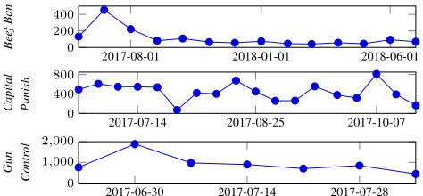
In this work, we use news articles on three topics that appeared in a 14 month period (June 2017 – July 2018). Within each topic we comparatively summarise news articles in different time periods to identify what has changed in that topic between the summarisation periods. To ensure our method works on a range of topics we chose substantially
different long running topics:Beef Ban– controversy over
the slaughter and sale of beef on religious grounds (1543 articles) is localised to a particular region, mainly Indian
subcontinent, whileGun Control– restrictions on carrying,
using, or purchasing firearms (6494 articles) andCapital
Punishment– use of the death penalty (7905 articles) are
2017-08-01 2018-01-01 2018-06-01
0 200 400
Beef
Ban
2017-07-14 2017-08-25 2017-10-07
0 400 800
Capital Punish.
2017-06-30 2017-07-14 2017-07-28
0 1,000 2,000
Gun
Contr
ol
Figure 3: Data volume over time for each topic
topical in various regions around the world. Figure 3 shows the number of new articles on each topic over time.
6
Experiments and Results
We evaluate approaches to comparative summarisation using both automatic and crowd-sourced human classification tasks. This choice stems from with our classification perspective (see §3.1), and has been used in the prototype selection literature (Bien and Tibshirani 2011; Kim, Khanna, and Koyejo 2016). Intuitively, a good set of prototype articles should uniquely identify a new article’s group.
Datasets and features. We empirically validate classifica-tion and prototype selecclassifica-tion methods on a well known USPS dataset (Bien and Tibshirani 2011; Kim, Khanna, and Koyejo
2016). USPS contains16×16grayscale handwritten digits
in 10 classes (i.e., digits 0 through 9). To reduce the dimen-sionality we use PCA, projecting the 256 dimensional image vectors into 39 features that explain 85% of the variance. The USPS dataset provides 7291 training and 2007 test im-ages. We generate another 9 random splits with exactly the same number of training and test images for the purposes of estimating confidence intervals.
In using the USPS dataset our aims are twofold. First, it shows the versatility of the method: the domain need not be text, collections need not be separated by time, and it operates with more than two classes. Indeed, by thinking of each digit
as agroup, our method can identify representative and diverse
examples of digits. Second, our method can be seen as a special kind of prototype selection for which the USPS dataset has been used as a standard benchmark (Bien and Tibshirani 2011; Kim, Khanna, and Koyejo 2016).
We further use the controversial news dataset described in §5 to evaluate comparative summarisation. We adopt the pre-trained GloVe-300 (Pennington, Socher, and Manning 2014) vector representation for each word, and then represent the article as an average of the word vectors from its the title and first 3 sentences – the most important text due to the inverted pyramid structure in news style (Pöttker 2003). This feature performs competitively in retrieval tasks despite its simplicity (Joulin et al. 2016). For each news topic, we generate 10 random splits with 80% training articles and 20% test articles for automatic evaluation. One of these splits is used for human evaluation.
1NN SVM
Capital Pun
Beefban
Guncontr
ol
USPS
2 4 8 16 2 4 8 16
0.4 0.5 0.6
0.4 0.5 0.6
0.4 0.5
0.4 0.5 0.6 0.7 0.8 0.9
number of prototypes
balanced accurac
y kmedoids
kmeans mmd−critic mmd−diff−grad mmd−div−grad nn−comp−greedy mmd−diff−greedy mmd−div−greedy
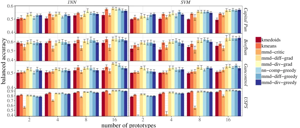
Figure 4: Comparative summarisation methods evaluated using the balanced accuracy of 1-NN (left) and SVM (right) classifiers. Each row represent a dataset. Error bars show 95% confidence intervals.
• nn-comp-greedyrepresents the nearest neighbour objective
Unn, optimised in a greedy manner.
• mmd-diffrepresents the difference of MMD objectiveUdiff.
mmd-diff-graduses gradient based optimisation while
mmd-diff-greedyis optimised greedily.
• mmd-div-gradandmmd-div-greedyare the gradient-based
and greedy variants of the diverse MMD objectiveUdiv.
with three baseline approaches:
• kmeansclusters with kmeans++ initialisation (Arthur and
Vassilvitskii 2007) found separately for each document
group. TheM cluster centers for each group are snapped
to the nearest data point using Equation 8.
• kmedoids(Kaufman and Rousseeuw 1987) clustering
algo-rithm with kmeans++ initialisation, computed separately for each document group. The medoids become the proto-types themselves.
• mmd-critic(Kim, Khanna, and Koyejo 2016) selects
proto-types using greedy optimisation ofMMD2and criticisms
by choosing points that deviate from the prototypes. The summary is selected from the unlabeled training set and consists of prototypes and criticisms in a one-to-one ratio. We use the Radial Basis Function (RBF) kernel when
applicable. The hyper-parameterγis chosen along with the
trade-off factorλ, and SVM soft marginCusing grid search
3 fold cross-validation on the training set. Note that 1NN
has no tunable parameters. Thegradoptimisation approach
uses the L-BFGS algorithm (Byrd et al. 1995), with initial
prototype guesses chosen by thegreedyalgorithm for news
dataset and K-means for USPS dataset.
6.1
Automatic Evaluation Settings
The controversial news dataset topics are divided into two groups of equal duration based on article timestamp. Note
that typically the number of documents in each time range is imbalanced. The USPS hand written digits dataset is divided into 10 groups corresponding to the 10 different digits. On each training split we select the prototypes for each group and then train an SVM or 1NN on the set of prototypes.
We measure the classifier performance on the test set using balanced accuracy, defined as the average accuracy of all classes (Brodersen et al. 2010). For binary classification
this is 12(TP
P + TN
N ), defined in terms of total positivesP,
total negatives N, true negatives TN, and true positives
TP. Balanced accuracy accounts for class imbalance, and
is applicable to both binary and multi-class classification tasks (whereas AUC and average precision are not). For all approaches, we report the mean and 95% confidence interval of the 10 random splits.
We report results on 2, 4, 8, or 16 prototypes per group – a small number of prototypes is necessary for the summaries to be meaningful to humans. This is in contrast to the hundreds of prototypes used by (Bien and Tibshirani 2011; Kim, Khanna, and Koyejo 2016), in automatic evaluations of the predictive quality of prototypes.
6.2
Automatic Evaluation Results
Figure 4 reports balanced accuracy for all methods using SVM and 1-NN across different datasets and numbers of prototypes. On the USPS dataset, most methods perform well.
The differences are small, if at all distinguishable.mmd-critic
performs poorly on USPS; this is because it does not guarantee a fixed number of prototypes per group, and sometimes misses a group all together. Note that this is very unlikely to occur with only 2 groups in the news dataset.
On the three news datasets, comparative summaries based
onnnandmmdobjectives are the best-performing approach
in 22 out of 24 evaluations (2 classifiers x 4 prototype sizes x
cases, they are the second-best with overlapping confidence intervals against the best (kmeans). Despite the lack of
opti-misation guarantees,gradoptimisation produces prototypes
of better quality in 15 out of 24 settings.
Generally, all methods produce better classification accu-racy as the number of prototypes increases. This indicates that the chosen prototypes do introduce new information that helps with the classification. In the limit, where all documents are selected as prototypes – a setting that is clearly unreason-able when summarisation is the goal – the performance is determined by the classifier alone. SVM achieves 0.763 on
Capital PunishmentandBeef Ban, 0.707 onGun Control,
while 1-NN achieves 0.762 onCapital Punishment, 0.763 on
Beef Banand 0.702 onGun Control. As seen in Figure 4 no
prototype selection method approaches this accuracy. This highlights the difficulty of selecting only a few prototypes to represent complex distributions of news articles over time.
6.3
Crowd-sourced Evaluation Settings
We conduct a user study on the crowd-sourcing platform
figure-eight2with two questions in mind: (1) using article
classification accuracy as a proxy, do people perform similarly to automatic evaluation? (2) how useful do people find the comparative summaries? This is an acid test on providing value to users who need comprehend large document corpora. Human evaluations in this work are designed to grade our method in a real world task: accurately identifying a news articles group (e.g. the month it is published) given only a few (4) articles from each month. The automatic evaluations in §6.2 are instructive proxies for efficacy, but inherently incomplete without human evaluation.
Generating summaries for the crowd. We present
sum-maries from four methodskmeans,nn-comp-greedy,
mmd-diff-greedy, andmmd-diff-grad– chosen because they perform
well in automatic evaluation and together form a cross-section of different method types. We opt to vary the groups of news articles being summarised by choosing many pairs of time ranges, since summaries on the same pair of groups (by definition) tend to be very similar or identical, which incurs
user fatigue. We use theBeef Bantopic because it has the
longest time range: June 2017 to July 2018 inclusive. The articles are grouped into each of the 14 months, and then 91 (i.e., 14 choose 2) pairs are formed. We take the top 10 pairs by performance according automatic evaluation using each of the four approaches, the union of these lead to 21 pairs. We pick top-performing pairs because preliminary human experiments showed that humans seem unable to classify
an article when automatic results do poorly (e.g.<0.65 in
balanced accuracy). Articles from each of the 21 pairs of months are randomly split into training and testing sets. We ask participants to classify six randomly sampled test articles. To reduce evaluation variance, all methods share the same test articles, different methods are randomized and are blind to workers. We record three independent judgments for each (test article, month-pair) tuple – totaling 1,512 judgments from 126 test questions over four methods. We also restrict
the crowd workers to be from India, whereBeef Banis locally
2https://www.figure-eight.com
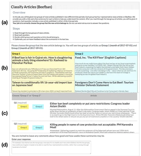
Figure 5: An example questionnaire used for crowd-sourced evaluation. It consists of: (a) instructions, (b) two groups of summaries, (c) question articles, and (d) a comment box for feedback. See §6.3.
relevant, and workers will be familiar with the people, places and organisations mentioned news articles.
Questionnaire design. Figure 5 shows the questionnaires we designed for human evaluation. Each questionnaire has 4 parts: (a) instructions, (b) two groups of prototypes, (c) test articles that must be classified into a group, and (c) a comment box for free-form feedback.
In the instruction (a), we explain that the two groups of representative articles (the prototypes for each time range) are articles from different time ranges and lay out the steps to complete the questionnaire. We ask participants not to use external sources to help classify test articles.
The two groups of prototype articles (b) are chosen by one
of the method being evaluated (e.g.,mmd-diff-gradorkmeans)
from articles in two different time ranges. Each group has four representative articles and each article has a title and a couple of sentences to help understand the content. We assign a different background colour to each group of summaries to give participants a visual guide.
Below the groups of summary articles are three questions (c), though for brevity only two are shown in Figure 5. Each question asks participants to decide which of the two time ranges a test article belongs to.
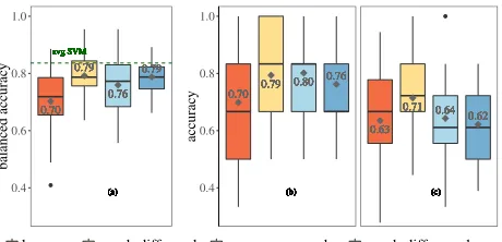
avg SVM avg SVM avg SVM avg SVM avg SVM avg SVM avg SVM avg SVM avg SVM avg SVM avg SVM avg SVM avg SVM avg SVM avg SVM avg SVM avg SVM avg SVM avg SVM avg SVM avg SVM avg SVM avg SVM avg SVM avg SVM avg SVM avg SVM avg SVM avg SVM avg SVM avg SVM avg SVM avg SVM avg SVM avg SVM avg SVM avg SVM avg SVM avg SVM avg SVM avg SVM avg SVM avg SVM avg SVM avg SVM avg SVM avg SVM avg SVM avg SVM avg SVM avg SVM avg SVM avg SVM avg SVM avg SVM avg SVM avg SVM avg SVM avg SVM avg SVM avg SVM avg SVM avg SVM avg SVM avg SVM avg SVM avg SVM avg SVM avg SVM avg SVM avg SVM avg SVM avg SVM avg SVM avg SVM avg SVM avg SVM avg SVM avg SVM avg SVM avg SVM avg SVM avg SVM avg SVM (a) (a) (a) (a) (a) (a) (a) (a) (a) (a) (a) (a) (a) (a) (a) (a) (a) (a) (a) (a) (a) (a) (a) (a) (a) (a) (a) (a) (a) (a) (a) (a) (a) (a) (a) (a) (a) (a) (a) (a) (a) (a) (a) (a) (a) (a) (a) (a) (a) (a) (a) (a) (a) (a) (a) (a) (a) (a) (a) (a) (a) (a) (a) (a) (a) (a) (a) (a) (a) (a) (a) (a) (a) (a) (a) (a) (a) (a) (a) (a) (a) (a) (a) (a) 0.76 0.79 0.79 0.70 0.76 0.79 0.79 0.70 0.76 0.79 0.79 0.70 0.76 0.79 0.79 0.70 0.76 0.79 0.79 0.70 0.76 0.79 0.79 0.70 0.76 0.79 0.79 0.70 0.76 0.79 0.79 0.70 0.76 0.79 0.79 0.70 0.76 0.79 0.79 0.70 0.76 0.79 0.79 0.70 0.76 0.79 0.79 0.70 0.76 0.79 0.79 0.70 0.76 0.79 0.79 0.70 0.76 0.79 0.79 0.70 0.76 0.79 0.79 0.70 0.76 0.79 0.79 0.70 0.76 0.79 0.79 0.70 0.76 0.79 0.79 0.70 0.76 0.79 0.79 0.70 0.76 0.79 0.79 0.70 0.4 0.6 0.8 1.0 balanced accurac y (b) (b) (b) (b) (b) (b) (b) (b) (b) (b) (b) (b) (b) (b) (b) (b) (b) (b) (b) (b) (b) (b) (b) (b) (b) (b) (b) (b) (b) (b) (b) (b) (b) (b) (b) (b) (b) (b) (b) (b) (b) (b) (b) (b) (b) (b) (b) (b) (b) (b) (b) (b) (b) (b) (b) (b) (b) (b) (b) (b) (b) (b) (b) (b) (b) (b) (b) (b) (b) (b) (b) (b) (b) (b) (b) (b) (b) (b) (b) (b) (b) (b) (b) (b) 0.80 0.76 0.79 0.70 0.80 0.76 0.79 0.70 0.80 0.76 0.79 0.70 0.80 0.76 0.79 0.70 0.80 0.76 0.79 0.70 0.80 0.76 0.79 0.70 0.80 0.76 0.79 0.70 0.80 0.76 0.79 0.70 0.80 0.76 0.79 0.70 0.80 0.76 0.79 0.70 0.80 0.76 0.79 0.70 0.80 0.76 0.79 0.70 0.80 0.76 0.79 0.70 0.80 0.76 0.79 0.70 0.80 0.76 0.79 0.70 0.80 0.76 0.79 0.70 0.80 0.76 0.79 0.70 0.80 0.76 0.79 0.70 0.80 0.76 0.79 0.70 0.80 0.76 0.79 0.70 0.80 0.76 0.79 0.70 (c) (c) (c) (c) (c) (c) (c) (c) (c) (c) (c) (c) (c) (c) (c) (c) (c) (c) (c) (c) (c) (c) (c) (c) (c) (c) (c) (c) (c) (c) (c) (c) (c) (c) (c) (c) (c) (c) (c) (c) (c) (c) (c) (c) (c) (c) (c) (c) (c) (c) (c) (c) (c) (c) (c) (c) (c) (c) (c) (c) (c) (c) (c) (c) (c) (c) (c) (c) (c) (c) (c) (c) (c) (c) (c) (c) (c) (c) (c) (c) (c) (c) (c) (c) 0.64 0.62 0.71 0.63 0.64 0.62 0.71 0.63 0.64 0.62 0.71 0.63 0.64 0.62 0.71 0.63 0.64 0.62 0.71 0.63 0.64 0.62 0.71 0.63 0.64 0.62 0.71 0.63 0.64 0.62 0.71 0.63 0.64 0.62 0.71 0.63 0.64 0.62 0.71 0.63 0.64 0.62 0.71 0.63 0.64 0.62 0.71 0.63 0.64 0.62 0.71 0.63 0.64 0.62 0.71 0.63 0.64 0.62 0.71 0.63 0.64 0.62 0.71 0.63 0.64 0.62 0.71 0.63 0.64 0.62 0.71 0.63 0.64 0.62 0.71 0.63 0.64 0.62 0.71 0.63 0.64 0.62 0.71 0.63 0.4 0.6 0.8 1.0 accurac y
kmeans mmd−diff−grad nn−comp−greedy mmd−diff−greedy
Figure 6: Classification accuracies for 21 pairs of summaries. (a) Automatic classification using prototypes (by SVM) on the
entire test set. The greenavg SVMline is the mean accuracy
of SVMs trained on the entire training set. (b) Automatic classification evaluated on 6 test articles per pair. (c) Human classification accuracy on 6 test articles per pair.
amongst the test questions. These ground truth questions are manually curated and reviewed if many workers fail on them. Each unit of work includes 4 questionnaires (of 3 questions each), one of which is a group of ground truth questions randomly positioned. Note that ground truth questions are only used to filter out participants and are not included in the evaluation results.
6.4
Crowd-sourced Evaluation Results
Worker profile.The number of unique participants answer-ing test questions ranged from 25 to 31 for each method, indicating that the results were not dominated a small number of participants. On average, participants spent 51 seconds on each test question and 2 minutes 33 seconds on each summary.
Quantitative resultsFigure 6 shows that on average crowd
workers with mmd-diff-gradsummaries classify an article
more accurately than summaries from other approaches by at
least 7%. The results are statistically significant withp <0.05
under a one sidedsign test; which applies because the 126
test questions where answered by three random people and we cannot assume normality. It also has the highest number
of consensus correct judgments (details in Appendix1).
mmd-diff-greedyperforms worse thanmmd-diff-grad.
We also compute the Fleiss Kappa statistic to measure
inter-annotator agreement. The statistics are: 0.418 forkmeans,
0.456 formmd-diff-grad, 0.435 fornn-comp-greedy, and 0.483
formmd-diff-greedyand a combined statistic of 0.451. All
statistics fall into the range of moderate agreement (Lan-dis and Koch 1977), which means the results we obtain in crowdsourced evaluations are reliable.
The good performance of gradient-based optimisation is surprising given greedy approaches are usually preferred in subset selection tasks, due to approximation guarantees for submodular objectives. One plausible explanation is that
early prototypes selected bygreedytend to cluster around
the first prototype, whereas the simultaneous optimisation
in grad tend to spread prototypes in feature space. With
only four prototypes being shown to users, diversity is an important factor for human classification. Previous studies of
greedymethods for prototype selection have used hundreds
of prototypes (Bien and Tibshirani 2011) – a setting in which the diversity of the early prototypes matters less – or used criticisms (Kim, Khanna, and Koyejo 2016) to improve diversity in tandem.
Comparing Figure 6 (a) – (c), automatic classifiers trained on both the entire training set and prototypes have higher classification accuracy than human workers across all methods. This observation indicates that using summaries to classify articles is difficult for humans. It could also indicate that humans use different features for article grouping, and word vectors alone may not capture those features.
Qualitative observations.Results from the optional free-form comments show that the participants found the classifi-cation difficulty to vary wildly. While some sets of articles were apparently easy to classify (e.g., “Group articles are distinct in their manner, among which all are articles are easy to determine."), other articles were difficult to classify (e.g., “Although two groups are clearly distinct, this one (news article) was pretty difficult to ascertain in which group it belongs to.") In some cases poor summaries seem to have made the task exceedingly difficult; e.g., “Q1, Q2, Q3 all are not belongs to group 1 and group 2 any topic I think." (quoted verbatim).
We found that the Beef Ban topic interested many of
our participants, with some expressing their views on the summarised articles, for example “Firstly we should define what is beef ..is it a cow or any animal?" and “It is a broad matter, what we should eat or not, it cannot be decided by government." (edited for clarity).
Participant comments also give some insight into what features were used to make classification. In particular, word and entity matching were frequently mentioned, a representa-tive user comment is “None of the questions match the given article, but I had to go by words used." All crowd-sourced evaluation results and comments are available in the dataset
github repository1.
7
Conclusion
We formulated the comparative document summarisation in terms of competing binary classifiers. This inspired new
MMDbased objectives amenable to both gradient and greedy
optimisation. Moreover, the setting enabled us to design effi-cient automatic and human evaluations to compare different objectives and optimisation methods on a new, highly
rele-vant dataset of news articles. We found that our newMMD
approaches, optimised by gradient methods, frequently out-performed all alternatives, including the greedy approaches currently favoured by the literature. Future work can include new use cases for comparative summarisation, such as authors or view points; richer text features; extensions to cross-modal comparative summarisation.
References
Arthur, D., and Vassilvitskii, S. 2007. k-means++: The
advantages of careful seeding. InACM-SIAM symposium on
Discrete algorithms.
Bien, J., and Tibshirani, R. 2011. Prototype selection for
interpretable classification. The Annals of Applied Statistics.
Brodersen, K. H.; Ong, C. S.; Stephan, K. E.; and Buh-mann, J. M. 2010. The balanced accuracy and its posterior
distribution. InInternational Conference on Pattern Recognition.
Byrd, R. H.; Lu, P.; Nocedal, J.; and Zhu, C. 1995. A limited
memory algorithm for bound constrained optimization.SIAM
Journal on Scientific Computing.
Carbonell, J., and Goldstein, J. 1998. The use of mmr, diversity-based reranking for reordering documents and
pro-ducing summaries. InACM SIGIR Conference on Research and
Development in Information Retrieval.
Garimella, K.; Morales, G. D. F.; Gionis, A.; and Math-ioudakis, M. 2018. Quantifying controversy on social media.
Transactions on Social Computing.
Gretton, A.; Borgwardt, K. M.; Rasch, M. J.; Schölkopf, B.;
and Smola, A. 2012. A kernel two-sample test. Journal of
Machine Learning Research.
Haghighi, A., and Vanderwende, L. 2009. Exploring content
models for multi-document summarization. InConference of
the North American Chapter of the Association for Computational Linguistics on Human Language Technology.
Huang, X.; Wan, X.; and Xiao, J. 2011. Comparative news
summarization using linear programming. InAnnual Meeting
of the Association for Computational Linguistics: Human Language Technologies.
Joulin, A.; Grave, E.; Bojanowski, P.; and Mikolov, T. 2016.
Bag of tricks for efficient text classification. arXiv preprint
arXiv:1607.01759.
Kaufman, L., and Rousseeuw, P. 1987.Clustering by means of
medoids. North-Holland.
Kim, B.; Khanna, R.; and Koyejo, O. O. 2016. Examples are not enough, learn to criticize! criticism for interpretability. In
Advances in Neural Information Processing Systems.
Landis, J. R., and Koch, G. G. 1977. The measurement of
observer agreement for categorical data.biometrics.
Li, L.; Zhou, K.; Xue, G.-R.; Zha, H.; and Yu, Y. 2009. Enhancing diversity, coverage and balance for summarization
through structure learning. InInternational Conference on World
Wide Web.
Li, J.; Li, L.; and Li, T. 2012. Multi-document summarization
via submodularity.Applied Intelligence.
Lin, H., and Bilmes, J. 2010. Multi-document summarization via budgeted maximization of submodular functions. In
Conference of the North American Chapter of the Association for Computational Linguistics on Human Language Technology.
Lin, H., and Bilmes, J. 2011. A class of submodular
func-tions for document summarization. In Annual Meeting of
the Association for Computational Linguistics: Human Language Technologies.
Lin, C.-Y., and Hovy, E. 2003. Automatic evaluation of
sum-maries using n-gram co-occurrence statistics. InConference of
the North American Chapter of the Association for Computational Linguistics on Human Language Technology.
Lin, C.-Y. 2004. Rouge: A package for automatic evaluation
of summaries. Text Summarization Branches Out.
Mirzasoleiman, B.; Badanidiyuru, A.; and Karbasi, A. 2016. Fast constrained submodular maximization: Personalized
data summarization. InInternational Conference on Machine
Learning.
Mitrovic, M.; Kazemi, E.; Zadimoghaddam, M.; and Kar-basi, A. 2018. Data summarization at scale: A two-stage
submodular approach. InInternational Conference on Machine
Learning.
Nemhauser, G. L.; Wolsey, L. A.; and Fisher, M. L. 1978. An analysis of approximations for maximizing submodular set
functions - i. Mathematical Programming.
Nenkova, A.; Passonneau, R.; and McKeown, K. 2007. The pyramid method: Incorporating human content selection
variation in summarization evaluation.ACM Transactions on
Speech and Language Processing.
Pennington, J.; Socher, R.; and Manning, C. 2014. Glove:
Global vectors for word representation. InEmpirical Methods
in Natural Language Processing.
Pöttker, H. 2003. News and its communicative quality: The
inverted pyramid - when and why did it appear?Journalism
Studies.
Ren, Z.; Inel, O.; Aroyo, L.; and De Rijke, M. 2016. Time-aware multi-viewpoint summarization of multilingual social
text streams. InACM International on Conference on Information
and Knowledge Management.
Rücklé, A., and Gurevych, I. 2017. Real-time news
summa-rization with adaptation to media attention. InRecent Advances
in Natural Language Processing, RANLP.
Schölkopf, B., and Smola, A. J. 2002.Learning with kernels.
MIT Press.
Simon, I.; Snavely, N.; and Seitz, S. M. 2007. Scene
sum-marization for online image collections. In International
Conference on Computer Vision.
Verkamp, J.-P., and Gupta, M. 2013. Five incidents, one theme: Twitter spam as a weapon to drown voices of protest. InUSENIX Workshop on Free and Open Communications on the Internet.
Wang, D.; Zhu, S.; Li, T.; and Gong, Y. 2012. Compara-tive document summarization via discriminaCompara-tive sentence
selection.ACM Transactions on Knowledge Discovery from Data.
Wei, K.; Iyer, R.; and Bilmes, J. 2015. Submodularity in
data subset selection and active learning. In International