Vol. 7, No. 3, 2015 Article ID IJIM-00610, 11 pages Research Article
Applying fuzzy wavelet like operator to the numerical solution of
linear fuzzy Fredholm integral equations and error analysis
F. Mokhtarnejad ∗, R. Ezzati †‡
————————————————————————————————–
Abstract
In this paper, we propose a successive approximation method based on fuzzy wavelet like operator to approximate the solution of linear fuzzy Fredholm integral equations of the second kind with arbitrary kernels. We give the convergence conditions and an error estimate. Also, we investigate the numerical stability of the computed values with respect to small perturbations in the first iteration. Finally, to show the efficiency of the proposed method, we present some test problems, for which the exact solutions are known.
Keywords: Fuzzy Fredholm integral equation; Fuzzy wavelet like operator; Successive approximation method.
—————————————————————————————————–
1
Introduction
F
uin physical problems as a result of the pos-zzy linear integral equations arise frequently sibility of super-imposing the effects due to sev-eral reasons. The most important contribution of the theory of fuzzy integral equations consists in the solution of fuzzy initial and boundary value problems. Also, the theory of fuzzy Volterra inte-gral equations makes it possible to solve an initial value problem for a linear fuzzy ordinary differ-ential equation of an arbitrary order [39].The concept of integration of fuzzy functions was introduced by Dubois and Prad [13] for the first time and then investigated by Goetschel and Vox-man [22], Kaleva [26], Matloka [29], Nanda [30] and others. One numerical method for solving fuzzy integrals is presented in [8]. The
fuzzy-∗Department of Mathematics, Karaj Branch, Islamic Azad University, Karaj, Iran.
†Corresponding author. ezati@ kiau.ac.ir
‡Department of Mathematics, Karaj Branch, Islamic Azad University, Karaj, Iran.
Riemann integral and its numerical integration was investigated by Wu in [36]. Some appli-cations of the fuzzy integral equations to con-trol models with fuzzy uncertainties are presented in[12]. In [15], the authors gave one of the applications of fuzzy integral for solving fuzzy Fredholm integral equation of the second kind (FFIE-2). On of the main fuzzy equations, ad-dressed by many researchers, is fuzzy Fredholm integral equation. Generally, the complexity of fuzzy integral equations hinders analytical solu-tions. Therefore, some numerical methods have been recently proposed to fuzzy fredholm inte-gral equation. The iterative techniques are ap-plied to FFIE-2 in [10, 16, 33, 38]. Friedman et al. [18] presented one successive approximations method for solving FFIE-2. Also, Friedman et al. [17] investigated numerical procedures for solv-ing FFIE-2 ussolv-ing the embeddsolv-ing method. Babo-lian et al. [7] used the Adomian decomposition method (ADM) to solve FFIE-2. Abbssbandy et al. [1, 27] obtained the solution of fuzzy Fred-holm integral equations by using the Nystrom
method. Recently,the authors used Lagrange in-terpolation [6], divided and finite differences [32], Bernstein polynomials [14, 31],Chebyshev inter-polation [9], Legendre wavelets [24], Splines in-terpolation [25],fuzzy Haar wavelets [35], and Galerkin type techniques [28]. Also, the authors of[36] proved the convergence of the method of successive approximations used to approximate the solution of nonlinear Hammerstein fuzzy in-tegral equations.
Here, by using fuzzy wavelet like operator, we propose a numerical approach for solving linear (FFIF-2):
˜
F(t) = ˜f(t)⊕λ⊙ ∫ b
a
K(x, t)⊙F˜(x)dx, (1.1)
where λ >0, K(x, t) is an arbitrary kernel func-tion over the square a ≤ x, t ≤ b and ˜f(t) is a fuzzy real valued function of t. Also, we present, the error estimation for approximating the solu-tion of linear FFIF-2.
This paper includes the following parts: In Sec-tion2, we review some elementary concepts of the fuzzy set theory and modulus of continuity. In Section3, the algorithm is given. In Section4, the convergence analysis is presented. In Section 5, the numerical stability with respect to the choice of the first iteration is demonstrated. In Section 6, we present two numerical examples for applica-bility of the proposed method to obtain numerical solution of linear FFIF-2 based on fuzzy wavelet like operator. Finally, Section 7 gives our con-cluding remarks.
2
Preliminaries
Definition 2.1 [21] A fuzzy number is a func-tionu:ℜ −→[0,1].with the following properties:
(i) u is normal, i.e. ∃x0∈ ℜ with u(x0) = 1,
(ii) u is a convex fuzzy set,
(iii) u is upper semi-continuous onℜ,
(iv) {x∈ ℜ:u(x)>0} is compact, where A de-notes the closure ofA.
The set of all fuzzy numbers is denoted byℜF.
Definition 2.2 [19] Suppose that u ∈ ℜF. The r-level set of u is denoted by [u]r = [u−(r), u(+r)]
and defined by [u]r = {x ∈ ℜ;u(x) ≥ r}, where
0 < r ≤ 1. Also, [u]0 is called the support of u and it is given as[u]0={x∈ ℜ;u(x)>0}. It fol-lows that the level sets ofuare closed and bounded intervals in ℜ.
It is well-known that the addition and multiplica-tion operamultiplica-tions of real numbers can be extended toℜF. In other words, foru, v∈ ℜF andλ∈ ℜ, we define uniquely the sum u⊕v and the product λ⊙u by
[u⊕v]r= [u]r+ [v]r,[λ⊙u]r =λ[u]r,∀r ∈[0,1],
where [u]r+ [v]r means the usual addition of two intervals (as subsets of ℜ) and λ[u]r means the usual product between a scalar and a subset of ℜ. We use the same symbol ∑ both for the sum of real numbers and for the sum ⊕ (when the terms are fuzzy numbers).
Definition 2.3 [19] An arbitrary fuzzy number is represented, in parametric form, by an ordered pair of functions (u(r), u(r)),0 ≤ r ≤ 1, which satisfy the following requirements:
(i) u(r) is a bounded left continuous nondecreas-ing function over [0,1],
(ii) u(r)is a bounded left continuous nonincreas-ing function over [0,1],
(iii) u(r)≤u(r), 0≤r ≤1.
The addition and scaler multiplication of fuzzy numbers inℜF are defined as follows:
(i) u⊕v= (u(r) +v(r), u(r) +v(r)),
(ii) (λ⊙u) =
{
(λu(r), λu(r)) λ≥0,
(λu(r), λu(r)) λ <0.
Definition 2.4 [20] For arbitrary fuzzy numbers u, v, the quantity
D(u, v) = sup
r∈[0,1]
max{|u(−r)−v−(r)|,|u(+r)−v+(r)| }
is the distance between u andv. It is proved that
(ℜF, D) is a complete metric space with the prop-erties ([23,34]).
(i) D(u⊕w, v⊕w) =D(u, v) ∀ u, v, w∈ ℜF,
(ii) D(k ⊙ u, k ⊙ v) = |k|D(u, v) ∀ u, v ∈ ℜF ∀k∈R,
(iii) D(u ⊕ v, w ⊕ e) ≤ D(u, w) +
Definition 2.5 [20] Let f, g : [a, b] → ℜF, be fuzzy real number valued functions. The uniform distance between f, g is defined by
D∗(f, g) = sup{D(f(x), g(x))|x∈[a, b]}.
Definition 2.6 [20] Let f : [a, b] → ℜF. f is fuzzy-Riemann integrable to J ∈ ℜF if for any ε >0, there existsδ >0such that for any division P ={[u, v];ξ} of [a, b] with the norms ∆(p)< δ, we have
D(∑
P
∗(v−u)⊙f(ξ), I)< ε,
where ∑∗ denotes the fuzzy summation. In this case it is denoted by I = (F R)∫abf(x)dx.
Definition 2.7 [3] A fuzzy real number valued function f :ℜ → ℜF is said to be continuous in x0 ∈ ℜ, if for each ε > 0 there is δ > 0 such that D(f(x), f(x0)) < ε, whenever x ∈ ℜ and |x−x0|< δ.We say thatf is fuzzy continuous on
ℜ if f is continuous at each x0 ∈ ℜ, and denote the space of all such functions by CF(ℜ).
Theorem 2.1 [2] If f, g : [a, b] ⊆ ℜ → ℜF are fuzzy continuous functions, then the function F
: [a, b] → ℜ+ defined by F(x) = D(f(x), g(x)) is continuous on[a, b], and
D (
(F R)
∫ b
a
f(x)dx,(F R)
∫ b
a
g(x)dx )
≤ ∫ b
a
D(f(x), g(x))dx.
Definition 2.8 [3] Let f : ℜ → ℜF. One call f a uniformly continuous fuzzy real number valued function, if and only if for any ϵ >0 there exists δ >0 whenever |x−y|≤δ;x, y ∈ ℜ, implies that D(f(x), f(y))≤ϵ. One denotes it asf ∈CU
F(ℜ).
Definition 2.9 [20, 4] Let f : ℜ → ℜF be a bounded function, then function
ωℜ(f, .) :ℜ+∪ {0} → ℜ+,
.
ωℜ(f, δ) = sup{D(f(x), f(y))| x, y∈ ℜ,
|x−y| ≤δ},where ℜ+ is the set of positive real numbers, is called the modulus of continuity of f onℜ.
Some properties of the modulus of continuity are presented below:
Theorem 2.2 [4] The following properties holds:
(1) D(f(x), f(y)) ≤ ω[a,b](f,|x − y|) for any x, y∈[a, b],
(2) ω[a,b](f, δ) is increasing function of δ,
(3) ω[a,b](f,0) = 0,
(4) ω[a,b](f, δ1+δ2) ≤ ω[a,b](f, δ1) + ω[a,b](f, δ2) for any δ1, δ2 ≥ 0, and f :ℜ → ℜF,
(5) ω[a,b](f, nδ) ≤ nω[a,b](f, δ) for any δ ≥
0, n∈N,and f :ℜ → ℜF,
(6) ω[a,b](f, λδ) ≤ [λ]ω[a,b](f, δ) ≤ (λ +
1)ω[a,b](f, δ) f or any δ, λ≥0,where [.] is the ceiling of the number, any f :ℜ → ℜF.
(7) If [c, d] ⊆ [a, b] then ω[c,d](f, δ) ≤ ω[a,b](f, δ).
In [5], the following theorem is proved.
Theorem 2.3 [4] Letf ∈CF(ℜ)and the scaling functionφ(x)a real-valued bounded function with suppφ(x) ⊆[−a, a],0 < a <+∞, φ(x)≥0, such that
+∞ ∑
j=−∞
φ(x−j) = 1
on ℜ. For k∈Z, x∈R, put
(Bkf)(x) := +∞ ∑
j=−∞ ∗
f( j
2k)⊙φ(2
kx−j),
which is a fuzzy-wavelet-like operator. Then
D((Bkf)(x), f(x))≤ωR(f, a
2k),
D∗((Bkf), f)≤ωR(f, a
2k),
for all x ∈ ℜ and k ∈ Z. If f ∈ CFU(ℜ), then as k → +∞ one gets ωℜ(f,2ak) → 0 and
3
The algorithm
Suppose that for all x ∈ [a, b] there exist j ∈ Z
such that 2mx −j ∈ [−a, a]. Now apply fuzzy wavelet like operator in the computation of the terms of the sequence of successive approxima-tions
˜
F0(t) = ˜f(t),
˜
Fk(t) = ˜f(t)⊕λ⊙ ∫ b
a
K(x, t)⊙F˜k−1(x)dx,
k≥1.Moreover we suppose that scaling function is as follow:
φ(x) =
1 −21 ≤x≤ 12,
0 o.w.
It obtains the following iterative algorithm: Step 0: There are introduced the a, b, m, ϵ and functions ˜f(t), λ, K(x, t).
Step 1:
˜
Y0,m(t) = ˜f(t),
Step 2: (the first iterative Step): Fork= 1 compute
˜
Yk,m(t) = ˜f(t)⊕λ⊙ ∫ b
a
K(x, t)⊙ ∞ ∑
j=−∞
˜
Yk−1,m( j
2m)⊙φ(2
mx−j)dx,
Step 3: (the generic iterative Step):
By induction fork∈N, k≥2,we use Step 2. Step 4:(a condition if ”do-while” type ):If
D∗( ˜Yk,m,Y˜k−1,m)< ϵ,
and
D∗( ˜Yk,m,f˜)< ϵ,
then we stop to this ”k” and computed at this last iterative retain the values ˜Yk,m(t, r) computed
|Y˜k,m(t, r)−f˜(t, r)|forr∈[0,1] andt= 0.5. Step 5: Print ”k”. STOP.
4
The convergence analysis
Definition 4.1 We say that the algorithm of successive approximations applied to the integral equation (1) is numerically stable with respect to the choice of the first iteration iff there exist a natural number k≥ 1, m∈Z and two constants K1, K2 >0 such that
D∗( ˜F ,Y˜k,m)≤K1ϵk1 +K2ϵm2 , f orϵ1 >0, ϵ2 >0.
Theorem 4.1 [22, 26] Let K(x, t) be continu-ous for a ≤ x, t ≤ b and f˜(t) a fuzzy con-tinuous function. If λ < M(b1−a), where M = max|K(x, t)|, a≤x, t≤b,then the iterative pro-cedure
˜
F0(t) = ˜f(t)
˜
Fk(t) = ˜f(t)⊕λ⊙ ∫ b
a
K(x, t)⊙F˜k−1(x)dx,
k ≥ 1 converges to the unique solution of above fuzzy integral equation. Specifically,
sup
a≤t≤b
D( ˜F(t),F˜k(t))
≤ Lk
1−Lasup≤t≤b
D( ˜F1(t),F˜0(t)),
where L=λM(b−a).
Theorem 4.2 Under the hypotheses of Theorem
4.1, we consider the following iterative procedure
˜
Y0,m(t) = ˜f(t),
˜
Yk,m(t) = ˜f(t)⊕λ⊙ ∫ b
a
K(x, t)⊙
∞ ∑
j=−∞
˜
Ym,k−1( j
2m)⊙φ(2
mx−j)dx, k≥1, m∈Z
where Y˜k,m ∈ C(ℜ), k ≥ 0, m ∈ Z the scaling functionφ(x) a real valued bounded function with suppφ(x) ⊆ [−a, a],0 < a < +∞, φ(x) ≥ 0, x ∈ ℜ such that
j=+∑∞
j=−∞
φ(x−j)≡1
on ℜ. Then
D( ˜F(t),Y˜k,m(t))≤ Lk
1−Lasup≤t≤b
D( ˜F1(t),F0˜(t))
+D( ˜F0(t),Y˜m,0(t)) + L
1−Lω( ˜Ymax, a
2m)), where
ω( ˜Ymax, a
2m) =max{ω( ˜Ym,0, a
2m),
ω( ˜Ym,1, a
2m), ω( ˜Ym,2, a
2m),· · ·, ω( ˜Ym,k, a
Table 1: Numerical results on the level sets for Example6.1
k=2, m=4 r-level |Yk,m−f| |Yk,m−f| k=4, m=16 |Yk,m−f| |Yk,m−f|
0.0 0.000000000 0.460913000 0.000000000 0.150909000
0.1 0.023045700 0.437868000 0.007545470 0.143364000
0.2 0.046091300 0.414822000 0.015090900 0.135818000
0.3 0.069137000 0.391776000 0.022636400 0.128273000
0.4 0.092182600 0.368731000 0.030181900 0.120727000
0.5 0.115228000 0.345685000 0.037727300 0.113182000
0.6 0.138276000 0.322639000 0.045272800 0.105637000
0.7 0.161320000 0.299594000 0.052818300 0.098091100
0.8 0.184365000 0.276548000 0.060363700 0.090545600
0.9 0.207411000 0.253502000 0.067909200 0.083000100
1.0 0.230457000 0.230457000 0.075454700 0.075454700
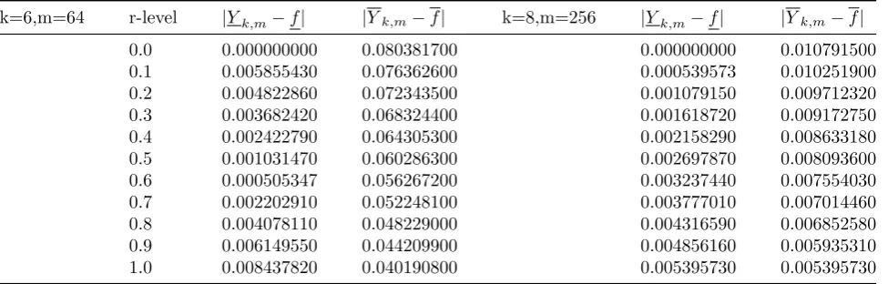
Table 2: Numerical results on the level sets for Example6.1
k=6,m=64 r-level |Yk,m−f| |Yk,m−f| k=8,m=256 |Yk,m−f| |Yk,m−f|
0.0 0.000000000 0.080381700 0.000000000 0.010791500
0.1 0.005855430 0.076362600 0.000539573 0.010251900
0.2 0.004822860 0.072343500 0.001079150 0.009712320
0.3 0.003682420 0.068324400 0.001618720 0.009172750
0.4 0.002422790 0.064305300 0.002158290 0.008633180
0.5 0.001031470 0.060286300 0.002697870 0.008093600
0.6 0.000505347 0.056267200 0.003237440 0.007554030
0.7 0.002202910 0.052248100 0.003777010 0.007014460
0.8 0.004078110 0.048229000 0.004316590 0.006852580
0.9 0.006149550 0.044209900 0.004856160 0.005935310
1.0 0.008437820 0.040190800 0.005395730 0.005395730
Table 3: Numerical results on the level sets for Example6.2
k=2,m=4 r-level |Yk,m−f| |Yk,m−f| k=4,m=16 |Yk,m−f| |Yk,m−f|
0.0 0.000000000 0.080045200 0.000000000 0.024050900
0.1 0.004002260 0.076043000 0.001202550 0.022848400
0.2 0.008004520 0.072040700 0.002405090 0.021645900
0.3 0.012006800 0.068038400 0.003607640 0.020443300
0.4 0.016009000 0.064036200 0.004810190 0.019240800
0.5 0.020011300 0.060033900 0.006127400 0.018038200
0.6 0.024013600 0.056317000 0.007215280 0.016835700
0.7 0.028015800 0.052029400 0.008417830 0.015633100
0.8 0.032018100 0.048027100 0.009620380 0.014430600
0.9 0.036020300 0.044024900 0.010822900 0.013228000
1.0 0.040022600 0.040022600 0.012025500 0.012025500
and
D∗( ˜F ,Y˜k,m)≤
Lk
1−LD
∗( ˜F1,F0˜) + L
1−Lω( ˜Ymax, a
2m)).
If Y˜k,m ∈ CFU(ℜ), then as m → +∞ we get ω( ˜Ymax,2am) → 0 , pointwise and uniformly with rates.
Proof.
D( ˜Fk(t),Y˜k,m(t)) =
D( ˜f(t)⊕λ⊙ ∫ b
a
K(x, t)⊙F˜k−1(x)dx,f˜(t)
⊕λ⊙ ∫ b
a
K(x, t)⊙ ∞ ∑
j=−∞
˜
Ym,k−1( j
2m)⊙φ(2
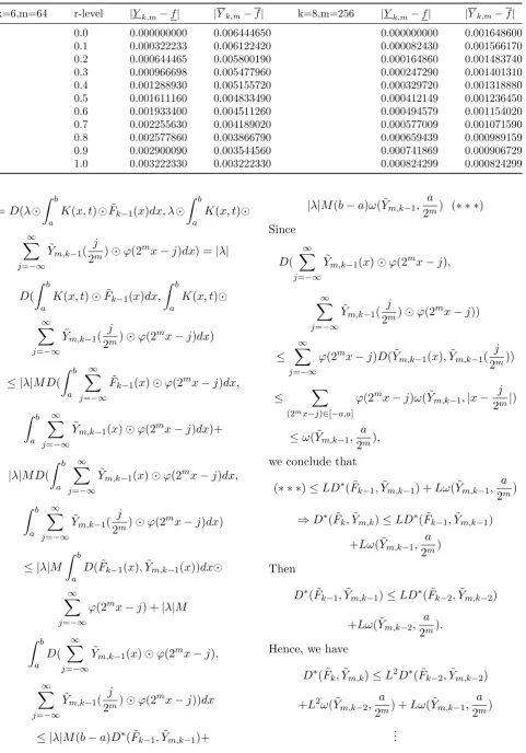
Table 4: Numerical results on the level sets for Example6.2
k=6,m=64 r-level |Yk,m−f| |Yk,m−f| k=8,m=256 |Yk,m−f| |Yk,m−f|
0.0 0.000000000 0.006444650 0.000000000 0.001648600
0.1 0.000322233 0.006122420 0.000082430 0.001566170
0.2 0.000644465 0.005800190 0.000164860 0.001483740
0.3 0.000966698 0.005477960 0.000247290 0.001401310
0.4 0.001288930 0.005155720 0.000329720 0.001318880
0.5 0.001611160 0.004833490 0.000412149 0.001236450
0.6 0.001933400 0.004511260 0.000494579 0.001154020
0.7 0.002255630 0.004189020 0.000577009 0.001071590
0.8 0.002577860 0.003866790 0.000659439 0.000989159
0.9 0.002900090 0.003544560 0.000741869 0.000906729
1.0 0.003222330 0.003222330 0.000824299 0.000824299
=D(λ⊙ ∫ b
a
K(x, t)⊙F˜k−1(x)dx, λ⊙ ∫ b
a
K(x, t)⊙
∞ ∑
j=−∞
˜
Ym,k−1( j
2m)⊙φ(2
mx−j)dx) =|λ|
D(
∫ b
a
K(x, t)⊙F˜k−1(x)dx, ∫ b
a
K(x, t)⊙
∞ ∑
j=−∞
˜
Ym,k−1( j
2m)⊙φ(2
mx−j)dx)
≤ |λ|M D(
∫ b
a
∞ ∑
j=−∞
˜
Fk−1(x)⊙φ(2mx−j)dx,
∫ b
a
∞ ∑
j=−∞
˜
Ym,k−1(x)⊙φ(2mx−j)dx)+
|λ|M D(
∫ b
a
∞ ∑
j=−∞
˜
Ym,k−1(x)⊙φ(2mx−j)dx,
∫ b
a
∞ ∑
j=−∞
˜
Ym,k−1( j
2m)⊙φ(2
mx−j)dx)
≤ |λ|M ∫ b
a
D( ˜Fk−1(x),Y˜m,k−1(x))dx⊙
∞ ∑
j=−∞
φ(2mx−j) +|λ|M
∫ b
a D(
∞ ∑
j=−∞
˜
Ym,k−1(x)⊙φ(2mx−j),
∞ ∑
j=−∞
˜
Ym,k−1( j
2m)⊙φ(2
mx−j))dx
≤ |λ|M(b−a)D∗( ˜Fk−1,Y˜m,k−1)+
|λ|M(b−a)ω( ˜Ym,k−1, a
2m) (∗ ∗ ∗)
Since
D( ∞ ∑
j=−∞
˜
Ym,k−1(x)⊙φ(2mx−j),
∞ ∑
j=−∞
˜
Ym,k−1( j
2m)⊙φ(2
mx−j))
≤ ∑∞
j=−∞
φ(2mx−j)D( ˜Ym,k−1(x),Y˜m,k−1( j
2m))
≤ ∑
(2mx−j)∈[−a,a]
φ(2mx−j)ω( ˜Ym,k−1,|x− j
2m|)
≤ω( ˜Ym,k−1, a
2m),
we conclude that
(∗ ∗ ∗)≤LD∗( ˜Fk−1,Y˜m,k−1) +Lω( ˜Ym,k−1, a
2m)
⇒D∗( ˜Fk,Y˜m,k)≤LD∗( ˜Fk−1,Y˜m,k−1)
+Lω( ˜Ym,k−1, a
2m)
Then
D∗( ˜Fk−1,Y˜m,k−1)≤LD∗( ˜Fk−2,Y˜m,k−2)
+Lω( ˜Ym,k−2, a
2m).
Hence, we have
D∗( ˜Fk,Y˜m,k)≤L2D∗( ˜Fk−2,Y˜m,k−2)
+L2ω( ˜Ym,k−2, a
2m) +Lω( ˜Ym,k−1, a
2m)
≤LkD∗( ˜F0,Y˜m,0) +Lω( ˜Ym,k−1, a
2m))+
L2ω( ˜Ym,k−2, a
2m)) +· · ·+L kω( ˜Y
m,0, a
2m)
So,
D∗( ˜Fk,Y˜m,k)≤LkD∗( ˜F0,Y˜m,0) +
Lω( ˜Ym,k−1, a
2m) +L 2ω( ˜Y
m,k−2, a
2m) +· · ·+
Lkω( ˜Ym,0, a
2m)
D∗( ˜Fk,Y˜m,k)≤LkD∗( ˜F0,Y˜m,0) +
(L+L2+L3+· · ·+Lk)ω( ˜Ymax, a
2m)
≤LkD∗( ˜F0,Y˜m,0) +
L(1−Lk)
1−L ω( ˜Ymax, a
2m),
Since
0< L <1⇒0< Lk<1⇒D∗( ˜Fk,Y˜m,k)
≤D∗( ˜F0,Y˜m,0) + L
1−Lω( ˜Ymax, a
2m).
Using properties of metrics space, we have:
D( ˜F(t),Y˜k,m(t))≤
D( ˜F(t),F˜k(t)) +D( ˜Fk(t),Y˜k,m(t))
Then
D∗( ˜F ,Y˜k,m)≤D∗( ˜F ,F˜k) +D∗( ˜Fk,Y˜k,m).
Hence
D∗( ˜F ,Y˜k,m)≤ Lk
1−LD ∗( ˜F
1,F˜0) +
D∗( ˜F0,Y˜m,0) + L
1−Lω( ˜Ymax, a
2m))
= L
k
1−LD
∗( ˜F1,F0˜ ) + L
1−Lω( ˜Ymax, a
2m)).
Remark 4.1 Since 0 < L < 1, it follows that limk→∞Lk = 0. In addition, from Theorem 15 we have when m→+∞ thenω( ˜Ymax,2am)→o So,
lim
k→∞,m→∞D
∗( ˜F ,Y˜k,m) = 0.
that shows the convergence of the method.
5
The numerical stability
anal-ysis
In order to investigate the numerical stability of the computed values with respect to small pertur-bations in the firs iteration we consider another first iteration term G0 ∈ CF(ℜ) such that there
exists ϵ > 0 for which D∗(F0, G0) < ϵ, for all t ∈ [a, b]. The new sequence of successive ap-proximation is:
˜
Gk,m(t) = ˜f(t)⊕λ⊙ ∫ b
a
K(x, t)⊙
∞ ∑
j=−∞
˜
Gm,k−1( j
2m)⊙φ(2
mx−j)dx,
k≥1, m∈Z
we redefine the new numerical iterative algorithm as follows:
˜
Y0,m(t) = ˜G0,m(t)
˜
Yk,m(t) = ˜f(t)⊕λ⊙ ∫ b
a
K(x, t)
⊙ ∑∞
j=−∞
˜
Ym,k−1( j
2m)⊙φ(2
mx−j)dx,
k≥1, m∈Z
Definition 5.1 We say that the method of suc-cessive approximation applied for solving the fuzzy linear FFIF-2 is numerically stable with re-spect to the choice of the first iteration term iff for each ϵ >0, such thatD∗( ˜Yk,m,Y˜k,m)< ϵ.
In order to obtain the numerical stability using given iterative procedure ˜Yk,m(t),Y˜k,m(t) fork≥
1, m∈Z and t∈[a, b] we have
D( ˜Yk,m(t),Y˜k,m(t))≤
D( ˜f(t)⊕λ⊙ ∫ b
a
K(x, t)⊙ ∞ ∑
j=−∞
˜
Ym,k−1( j
2m)
⊙φ(2mx−j)dx, ,f˜(t)⊕λ⊙ ∫ b
a
K(x, t)⊙
∞ ∑
j=−∞
˜
Ym,k−1( j
2m)⊙φ(2
≤D( ˜f(t),f˜(t)) +D(λ⊙ ∫ b
a
K(x, t)
⊙ ∑∞
j=−∞
˜
Ym,k−1( j
2m)⊙φ(2
mx−j)dx,
λ⊙ ∫ b
a
K(x, t)⊙ ∞ ∑
j=−∞
˜
Ym,k−1( j
2m)⊙φ(2
mx−j)dx)
≤ |λ|M ∫ b
a
D( ˜Ym,k−1( j
2m),Y˜m,k−1( j
2m))dx
≤ |λ|M(b−a)D( ˜Ym,k−1( j
2m),Y˜m,k−1( j
2m))
Then
D( ˜Ym,k−1(t),Y˜m,k−1(t))≤
(|λ|M(b−a))2D( ˜Ym,k−2( j
2m),Y˜m,k−2( j
2m))
.. .
D( ˜Yk,m(t),Y˜k,m(t))≤
(|λ|M(b−a))kD( ˜Ym,0( j
2m),Y˜m,0( j
2m))
D∗( ˜Yk,m,Y˜k,m)≤(|λ|M(b−a))kD∗( ˜Ym,0,Y˜m,0)
regarding to
D∗( ˜Ym,0,Y˜m,0) =D∗( ˜F0,G0˜ ,m)< ϵ
we deduce that
D∗( ˜Yk,m,Y˜k,m)≤ϵ(|λ|M(b−a))k
and since (|λ|M(b−a)) < 1, we conclude that the stability of the numerical method is proved. Indeed we have
limk→∞D∗( ˜Yk,m,Y˜k,m) = 0.
6
Numerical Examples
In this section, we apply the proposed method in Section 3 for solving the fuzzy linear FFIE-2 in some examples . We compare numerical results with exact solutions. Also, we apply the following scaling function
φ(x) =
1 −21 ≤x≤ 12,
0 o.w.
Example 6.1 Consider the following fuzzy Fred-holm integral equation
˜
F(t) = ˜f(t)⊕(F R)
∫ 1
0
k(x, t)⊙F˜(x)dx,
˜
f(t) = (f(t, r), f(t, r) =
((t+ 1)r−7r(1 +t2)/12,
(t+ 1)(2−r)−7(2−r)(1 +t2)/12),
t, r∈[0,1],
k(x, t) =t2/(1 +x2), t, x∈[0,1]
by exact solution F˜(t) = (F(t, r), F(t, r)) = ((t+ 1)r,(t+ 1)(2−r)), t, r∈[0,1].By using proposed algorithm in Section 3, we present approximate solution to this example in t = 0.5 for different values of k ,m in Tables 1, 2.
Example 6.2 Consider the following fuzzy Fred-holm integral equation
˜
F(t) = ˜f(t)⊕(F R)
∫ 1
0
k(x, t)⊙F˜(x)dx,
˜
f(t) = (f−(t, r), f−(t, r) =
(tr−5/52r−t2r/26,
2t−rt−t2/13+t2r/26−10/52+5r/42),
t, r∈[0,1],
k(x, t) = (t2+x2+ 2)/13, t, x∈[0,1]
by exact solution
˜
F(t) = (F−(t, r), F−(t, r)) = (tr, t(2−r)),
t, r∈[0,1].
By using proposed algorithm in Section 3, we present approximate solution to this example in
t= 0.5 for different values of k ,m in Tables3,4.
7
Conclusion
References
[1] S. Abbasbandy, E. Babolian, M. Alavi, Nu-merical method for solving linear fredholm fuzzy integral equations of the second kind, Chaos Solutions an Fractals 31 (2007) 138-146.
[2] G. A. Anastassiou, Rate of convergence of fuzzy neural network operators, univari-ate case, Journal of Fuzzy Mathematics 10 (2002) 755-780.
[3] G. Anastassiou, Quantitative Approxima-tions, Chapman and Hall/CRC, Boca Raton, Fla, USA, (2001).
[4] G. A. Anastassiou, Fuzzy Mathematics: Ap-proximation Theory, vol. 251 of Studies in Fuzziness and Soft Computing, Springer, Berlin, Germany, (2010).
[5] G. A. Anastassiou, Fuzzy wavelet type op-erators, Nonlinear Functional Analysis and Applications 2 (2004) 251269 .
[6] M.A.F.Araghi, N. Parandin, Numerical so-lution of fuzzy Fredholm integral equations by the Lagrange interpolation based on the extension principle, Soft Comput. 15 (2011) 24492456.
[7] E. Babolian, H. Sadeghi Goghary, S. Abbasbandy, Numerical solution of linear Fredholm fuzzy integral equa-tions of the second kind by Adomian method,Appl.Math.Comput. 161 (2006) 733-744.
[8] K. Balachandran, P. Prakash, Existence of solutions of nonlinear fuzzy Volterra-Fredholm integral equations, Indian J. Pure Appl. Math. 33 (2002) 329-343.
[9] M. Barkhordari Ahmadi, M . Khezerloo,
Fuzzy bivariate Chebyshev method for solving fuzzy VolterraFredholm integral equations, Int. J. Industrial Math. 3 (2011) 6777 .
[10] B. Bede, S. G. Gal, Quadrature rules for integrals of fuzzy-number-valued functions, Fuzzy Sets and Systems 145 (2004) 359-380 .
[11] A. M. Bica, Algebraic structures for fuzzy numbers from categorial point of view, Soft Computing 11 (2007)1099-1105 .
[12] P. Diamond, Theory and applications of fuzzy Volterra integral equations, IEEE Trans. Fuzzy Syst. 10 (2002) 97102.
[13] D. Dubois, H. Prade,Towards fuzzy differen-tial caculus, Fuzzy Sets and Systems 8 (1982) 225-233.
[14] R. Ezzati, S. Ziari, Numerical solution and error estimation of fuzzy Fredholm integral equation using fuzzy Bernstein polynomials, Aust. J. Basic Appl. Sci. 5 (2011) 20722082.
[15] M. Friedman, M. Ma, A. Kandel,Numerical methods for calculating the fuzzy integral, Fuzzy Sets and Systems 83 (1996) 57-62.
[16] M. Friedman, M. Ma, A. Kandel, On fuzzy integral equations, Fund. Inform. 37 (1999) 89-99, .
[17] M. Friedman, M. Ma, A. Kandel, Numer-ical solutions of fuzzy differential and inte-gral equations, Fuzzy Sets and Systems 106 (1999) 35-48.
[18] M. Friedman, M. Ma, A. Kandel, Solutions to fuzzy integral equations with arbitrary ker-nels, International Journal of Approximate Reasoning 20 (1999) 249-262.
[19] M. Friedman, M. Ming, and A. Kandel, Nu-merical methods for calculating the fuzzy in-tegral, Fuzzy Sets and Systems 83 (1996) 57-62.
[20] S. G. Gal, Approximation theory in fuzzy setting, in Handbookof Analytic-Computational Methods in Applied Mathe-matics, G. Anastassiou, Ed, Chapman and Hall/CRC, Boca Raton, Fla, USA, (2000) 617-666.
[21] R. Goetschel, W. Voxman,Elementary fuzzy calculus,Fuzzy Sets and Systems, 18 (1986) 31-43.
[23] C. Wu, Z. Gong, On Henstock integral of fuzzy-numbervalued functions, Fuzzy Sets and Systems 120 (2001) 523-532.
[24] H. Sadeghi Goghary,M. Sadeghi-Goghary,Two computational methods for solving linear Fredholm fuzzy integral equation of the second kind, Appl. Math. Comput. 182 (2006) 791796.
[25] Y. Jafarzadeh, Numerical solution for fuzzy Fredholmi ntegral equations with upper-bound on error by splines interpolation, Fuzzy Inf. Eng. 3 (2012) 339347.
[26] O. Kaleva, Fuzzy differential equations, Fuzzy Sets and Systems 24 (1987) 301-317 .
[27] M. Khezerloo,T. Allahviranloo, S. Salahshour, M. KhorasaniKiasari, S. HajiGhasemi,Application of Gaussian quadratures in solving fuzzy Fredholm integral equations, in: Information Pro-cessing and Management of Uncertainty inKnowledge-Based Systems. Applications, in: Communications in Computer and Information Science 81 (2010) 481490.
[28] T. Lotfi, K. Mahdiani,Fuzzy Galerkin method for solving Fredholm integral equa-tions with error analysis, Int. J. Industrial Math. 3 (2011) 237249.
[29] M. Matloka,On fuzzy integral, proc.2nd pol-ish symp, on interval and fuzzy Mathemat-ics,Politechnika poznansk Fuzzy, 167-170.
[30] S. Nanda,On integration of fuzzy mappings, Fuzzy Sets and Systems 32 (1989) 95-101.
[31] M. Mosleh. M. Otadi, Numerical solution of fuzzy integral equations using Bernstein poly-nomials, Aust. J. Basic Appl. Sci. 5 (2011) 724728.
[32] N. Parandin, M. A. FaborziAraghi,The nu-merical solution of linear fuzzy Fredholm in-tegral equations of the second kind by using finite and divided differences methods, Soft Comput. 15 (2010) 729741 .
[33] J. Y. Park, S. Y. Lee, J. U. Jeong, The ap-proximate solution of fuzzy functional inte-gral equations, Fuzzy Sets and Systems 110 (2000) 79-90 .
[34] C. X. Wu, M. Ma, Embedding problem of fuzzy number space, Fuzzy Sets and Systems 44 (1991) 33-38 .
[35] S. Ziari, R. Ezzati, S. Abbasbandy, Numer-ical solution of linear fuzzy Fredholm inte-gral equations of the second kind using fuzzy Haar wavelet , Commun. Comput. Inf. Sci. 299 (2012) 7989.
[36] H. C. Wu, The fuzzy Riemann integral and its numerical integration , Fuzzy Sets and Systems 110 (2000) 1-25.
[37] A. M. Bica, C. Popescu,Approximating the solution of nonlinear Hammerstein fuzzy integral equations, Fuzzy Sets and Sys-tems 2013 .http://dx.doi.org/10.1016/ j.fss2013,08.005.
[38] R. Ezzati, S. Ziari,Numerical solution of nonlinear fuzzy Fredholm integral equations using iterative method, Applied Mathemat-ics and Computations 225 (2013) 3342.
[39] L. Sebastian, Some problems in integral equations using fuzzy set theory, Ph.D The-sis, 2014.
Fatemeh Mokhtarnejad was born in Bonab, Iran, in 1981. She re-ceived B.S. in applied mathemat-ics in 2004 and M.S. in 2007 from Tabriz Payame Noor University, Tabriz, Iran. She is a Senior Ph.D student at Faculty of Sciences in Is-lamic Azad University, Karaj Branch, Iran. Her main research interest is fuzzy mathematics es-pecially, on numerical solution of fuzzy integral equations.