ISSN: 2374-2348 (Print), 2374-2356 (Online) Copyright © The Author(s).All Rights Reserved. Published by American Research Institute for Policy Development DOI: 10.15640/arms.v7n1a1 URL: https://doi.org/10.15640/arms.v7n1a1
Bases of software for computer simulation and multivariante prediction of economic even
at uncertainty conditions on the base of n-component piecewise-linear
economic-mathematical models in m-dimensional vector space
Azad Gabil oglu Aliyev
1Abstract
For the last 15 years in periodic literature there has appeared a series of scientific publications that has laid the foundation of a new scientific direction on creation of piecewise-linear economic-mathematical models at uncertainty conditions in finite dimensional vector space. Representation of economic processes in finite-dimensional vector space, in particular in Euclidean space, at uncertainty conditions in the form of mathematical models in connected with complexity of complete account of such important issues as: spatial in homogeneity of occurring economic processes, incomplete macro, micro and social-political information; time changeability of multifactor economic indices, their duration and their change rate. The above-listed one in mathematical plan reduces the solution of the given problem to creation of very complicated economic-mathematical models of nonlinear type. In this connection, it was established in these works that all possible economic processes considered with regard to uncertainty factor in finite-dimensional vector space should be explicitly determined in spatial-time aspect. Owing only to the stated principle of spatial-time certainty of economic process at uncertainty conditions in finite dimensional vector space it is possible to reveal systematically the dynamics and structure of the occurring process. In addition, imposing a series of softened additional conditions on the occurring economic process, it is possible to classify it in finite-dimensional vector space and also to suggest a new science-based method of multivariant prediction of economic process and its control in finite-dimensional vector space at uncertainty conditions, in particular, with regard to unaccounted factors influence.
Keywords: Finite-dimensional vector space; Unaccounted factors; Unaccounted parameters influence function; Principle of certainty of economic process in fine-dimensional space; Multi alternative forecasting; Principle of spatial-time certainty of economic process at uncertainty conditions in fine-dimensional space; Piecewise-linear economic-mathematical models in view of the factor of uncertainty in finite-dimensional vector space; Piecewise-linear vector-function; 3-Dimensional Vector Space; 3-Component Piecewise-Linear Economic-Mathematical Model in 3-Dimensional Vector Space; Actions algorithm computer modeling and multi-variant prediction of economic event at uncertainty conditions on the base of 2 and 3-component piecewise-linear economic-mathematical models in m–dimensional vector space
I. Introduction. Formulation of the problem
Development of modern society is characterized by the increase of technical level, complication of organizational structure of production, intensification of social division of labour, making high demands on planning and economic management methods-different optimization models and optimization methods based on the use of mathematical simulation find effective application by solving practical operational problems. Today, newest achievements of mathematics and up-to-date calculating engineering find wider application in economic investigations and planning. According to the basic conditions, the simulation process stages acquire their specific character.
1.1 Statement of economic problem and its quality analysis
The given stage means explicit formulization of the problem’s essence, accepted assumptions. This stage includes distinction of the most important features and properties of the modeled object and its abstraction from the secondary ones; study of the structure and basic dependences connecting its elements; formulation of conjectures (even if preliminary ones), explaning the behavior and development of the object.
1.2. Construction of mathematical model
This stage is the stage of formalization of an economic problem, its expressions in the form of concrete mathematical dependences and relations (functions, equations, inequalities and etc.). Usually, at first the basic construction (type) of a mathematical model is determined, then the details of this construction (concrete list of variables and parameters, connection forms) are specified. It is incorrect to assume that the more facts takes into account a model, the best it “works” and gives best results. We can say the same on such characteristics of complexity of the model as the used forms of mathematical dependences (linear and nonlinear), accounting of accidental nature and uncertainty factors and so on. Superfluous complexity and awkwardness of the model makes difficult the investigation process. It is necessary to take into account not only real possibilities of information and software but also to compare simulation expenditure with the obtained efficiency (by increasing the complexity of the model, increase of expenditures may exceed the efficiency increase). Intercom parison of two systems of scientific knowledges i.e. economic and mathematical ones are realized in the process of construction of the model. It is natural to try to get a model belonging to the well studied class of mathematical problems. Often it is succeeded to do it by simplifying initial premises of the model that don’t distort the essential features of the modeled object. However the situation when the formalization of the economic problem reduces to the mathematical structure unknown earlier, is also possible.
1.3. Mathematical analysis of the model
The goal of this stage is elucidation of general properties of the model. Here truly mathematical investigation methods are used. The most important moment is to prove the existence of solutions in the formulated model (existence theorem). If it turns out well to prove that a mathematical problem has no solution, then the necessity in the subsequent work on the initial variant of the model falls away then either the statement of the economic problem or the ways of its mathematical formalization should be corrected. By analytic investigation of the model such questions as for example, if the solution is unique, which variables (unknown ones) may appear in the solution, what relations will be between them, in what limits and under which initial conditions they change, what tendencies of their change and etc. Analytic investigation of the model compared with empiric (numerical) one has the advantage that the obtained conclusions remain valid for different concrete values of external and internal parameters of the model. As the economic-mathematical simulation develops and gets complicated, its separate stages are isolated into specialized investigation fields, the difference between theoretical-analytical and applied models increases, differentiation of models by the levels of abstraction and idealization happens. Theory of mathematical analysis of economics models has been developed into a special branch of contemporary mathematics to mathematical economics. The models studied within mathematical economics loose direct connection with economic reality; they exceptionally deal with idealized economic objects and situations. By constructing such models, the chief principle is not so much approximation to reality as to obtain a possible great number of analytic results by means of mathematical proofs. The value of these models for economic theory and practice is that they serve as a theoretical basis for applied type models. Preparation and processing of economic information and development of software of economic problems (creation of data base and information banks, program of computer-aided construction of models and program service for economists-users) become independent fields of investigations.
1.4. Preparation of input information
Simulation presents rigid requirements to the information system. At the same time, real possibilities of information receipt restricts the choice of models intended for practical use. Not only principal possibility of information preparation (for certain periods) but also expenditures for preparation of appropriate information areas is taken into account. These expenditures should not exceed the efficiency from the use of additional information. The methods of probability theory, theoretical and mathematical statistics are widely used in the course of preparation of information. Under system economic-mathematical simulation the initial information used in one models, is the result of functioning of other models.
In this stage, the algorithms for numerical solution of the problem are worked out, the programs in ECM are composed and calculations are conducted. Difficulties of this stage are stipulated first of all by the great size of economical problems, by necessity of processing of considerable information areas. Usually, calculations on economic-mathematical model are of multivariant character. Owing to high speed of contemporary ECM we can conduct numerous “model” experiments studying “behavior” of the model under different changes of some conditions. The investigations conducted by numerical methods may essentially complement the results of analytic investigation, and for a lot of models it is a uniquely realizable one.
6. Analysis of numerical results and their application
On the final stage their arises a question on correctness and completeness of simulation, on degree of practical applicability of the latters. Mathematical verification methods may elucidate incorrect constructions of the model and by the same token contract the class of potentially tame models. Informal analysis of theoretical conclusion and numerical results obtained by means of the model, their comparison by the available knowledges and facts of reality also allow to reveal the short-comings of the economic problem statement, constructed mathematical model and its software.
Introduction of computer-aided systems of economic information processing allows to lower essentially the expenditures connected with data processing, to increase labour productivity of the labour of the workers in the field of economics, improve relations between different subdivisions of enterprises. At present, there is a great mass of software intended for application in the field of economics, but regretfully, often it is necessary to “adjust” the ready made software under individual features of the enterprise even if these programs stood the test by time. However, the arising difficulties of calculating character require the creation of special software for computer programming and creation of an action algorithm for economic processes at uncertainty conditions in finite-dimensional vector space.
In this connection, in [1,2,7,13-15], by means of 2-component piecewise linear economic-mathematical models with regard to unaccounted factors a special program is developed for computer modeling for numerical construction and definition of multivariant prediction quantities of economic event in many-dimensional vector space, in particular, in two, three and four-dimensional vector spaces. The scientific results obtained in these works compose necessary theoretical and calculation instrument for creating a principally new, perspective software for computer modeling by constructing and multivariant prediction of economic state by means of piecewise linear economic-mathematical models with regard to unaccounted factors influence in m –dimensional vector space.
In this article, the developed software algorithms for constructing two-component piecewise-linear model and for multivariant prediction of economic event at uncertainty conditions in m-dimensional vector space will be stated on the base of the Matlab program, and a number of numerical examples will be given. A packet of programs will be suggested, a numerical analysis of multivariant prediction of economic event at uncertainty conditions will be suggested.
II. Materials and methods.
Development of software for computer modeling and multi-variant prediction of economic event at uncertainty conditions on the base of 2-component piecewise-linear economic-mathematical models in m– dimensional vector space
2.1. Actions algorithm for computer modeling by constructing 2-component piecewise-linear economic-mathematical models
In this article, on the basis of the Matlab program we’ll suggest an algorithm and numerical calculation method for numerical construction of 2-component piecewise-linear economic-mathematical models in m-dimensional vector space. It should be noted that the Matlab program has its restrictive properties that compels us to introduce some additional denotation and adhere to certain proper sequence in calculation operations. According to the suggested theory [1-4,6-9,11,13-15], for the case of 2-component piecewise-linear vector function in m-dimensional vector space we write the min equations and mathematical expressions that are subjected to numerical programming.
Let in m-dimensional vector space Rm a statistical table describing some economic process in the form of
points (vectors) set {an}
)
a
-a
(
μ
a
z
1
1 1
2
1
(1))
z
-a
(
μ
z
z
1 k11 3 2 k 1 2
(2)where
z
1
z
1(z
11,
z
12,
z
13,...z
1m)
and
z
2
z
2(z
21,
z
22,
z
23,...z
2m)
are the equations of the first and second piecewise-linear straight lines in m-dimensional vector space. The vectorsa
1(a
11,
a
12,
a
13,...,
a
1m)
,)
a
,...,
a
,
a
,
(a
a
a
2
2 21 22 23 2m
and
a
3
a
3(a
31,
a
32,
a
33,...,
a
3m)
are the given points (vectors) in m-dimensional space, of the form:m 1m 3 13 2 12 1 11
1
a
i
a
i
a
i
...
a
i
a
, m 2m 3 23 2 22 1 212
a
i
a
i
a
i
...
a
i
a
(3)m 3m 3 33 2 32 1 31
3
a
i
a
i
a
i
...
a
i
a
Here
μ
1≥
0
andμ
2≥
0
are arbitrary parameters, k11
z
is the intersection point of the straight lines z1
and
z
2
.
The goal of the investigation is the following. Giving the approximative points
a
1,a
2,a
3 and also the values of the parameters *1 k
1
μ
μ
1
and *2 k
2
μ
μ
2
to develop a computer calculation algorithm of the followingequations and mathematical expressions in m–dimensional vector space:
)
-(
2 11 1
1 1
1
a
a
a
z
k
k
)
)(
(
)
(
1 2 1 3 2 1 3 2 1 1 1 1 2 1 2a
a
z
a
z
a
k k k k k
)
-(
2 11 1
2 1
2
a
a
a
z
k
k
)
(
)
(
)
)(
(
)
(
1 1 1 1 2 1 2 1 3 2 1 3 1 3 1 3 1 1 1 2 k k k k k k kz
a
z
a
a
a
z
a
z
z
1 2 1 2 1 2 1 2 1 1 1 1 1 1 1 1 2 , 1 -) -)( -( k k k k k k k k z z z z z z z zсos
) -( -) -( 1 1 1 1 1 1 2 11 2 1
1 2 1 a z z a z a a
A k k
k k k
1 k 1 1 2 1 1 1 1 1 1 k 1 3 1 1 2 1 2 2-)
-(
)
-(
--
1 1 2 1 2 2 1 1 2 2 1 2a
z
a
a
a
z
z
z
z
z
z
a
z
z
k kk k k k k k k k
2 , 1 2 2 , 1 22
(
,
)
сos
)]}
,
(
1
[
1
{
2 2 1,21 2
2
z
A
z
k)
-(
2 11
1
a
1a
a
2 k 1 3
1 2 k 1 3 1
1 2
)
(
)
)(
(
)
(
1 1 1
z
a
a
a
z
a
k
) (
-) (
) (
1 1 1
1 k 1 1 2
1 1
1 1
1 1
a z z
a z a a
A k k
1 k 1 1 2
1 1 1
1 1 1
k 1 3 1 1
1 1
2 1
2
-)
-(
)
-(
-)
(
1 1
1 1 1
1
a
z
a
a
a
z
z
z
z
z
z
a
z
z
kk k
k
2 , 1 1
2 1
2
(
)
(
)
Cos
)]}
(
1
)[
(
1
{
)
(
z
2
1
z
1
A
1
2
1
(4) Introduce the following denotation:
1
1
a
a
;a
2
a
2
; a3 a3;
1 m1;1
1
1
1
m
k
k
; 21
2
1
m
k
k
, 11
1
1
z
k
z
k
, 2 1 2
1 z k
zk ;
2
2
22
z
k
z
k
;
z
1
z
1
;
2
m
2
; 2 2 22 m k
k
, A(
1)Am1,2
2
La
,
2(
1)
La
2
m
1
;1
2
)
(
)
,
(
2 12 2 12
w
m
, z2 z2, z2(
1)z2m1. (5)Using the introduced denotation (5), for the system (4) compose a program for numerical construction of 2-component piecewise-linear economic-mathematical models with regard to unaccounted factors influence in m-dimensional vector space in the Matlab program in the following form [1,2,7,13-15]:
a1=[a11 a12 a13 …a1m] a2=[a21 a22 a23 …a2m] a3=[a31 a32 a33 …a3m] m1k1=(m1)*
m2k2=(m2)* for m1=J1: J2 :J3 z1k1=a1+m1k1*(a2-a1);
m1k2=m1k1+m2k2*((a3-z1k1)*(a3-z1k1)')/ ((a3-z1k1)*(a2-a1)');
z1k2=a1+m1k2*(a2-a1);
z2k2=z1k1+(m1k2-m1k1)*((a3-z1k1)*(a2-a1)')/((a3-z1k1)*(a3-z1k1)')*(a3-z1k1); cosa12=((z1k2-z1k1)*(z2k2-z1k1)')/(sqrt((z1k2-
-z1k1)*(z1k2-z1k1)')*sqrt((z2k2-z1k1)*(z2k2-z1k1)'))
A=(m1k1-m1k2)*(sqrt((a2-a1)*(a2-a1)')*sqrt((z1k1-a1)*(z1k1-a1)'))/(z1k2*(z1k1-a1)'); p1=m2k2/(m1k1-m1k2);
p2=(sqrt((z1k2-z1k1)*(z1k2-z1k1)')*sqrt((a3-z1k1)*(a3-z1k1)'))/(z1k2*(z1k2-z1k1)'); p3=(z1k2*(z1k1-a1)')/(sqrt((a2-a1)*(a2-a1)')*sqrt
((z1k1-a1)*(z1k1-a1)')); La2=p1*p2*p3; w2=La2*cosa12;
z2=z1k2*(1+A*(1+w2)); z1=a1+m1*(a2-a1)
m2=(m1-m1k1)*(((a3-z1k1)*(a2-a1)')/((a3-z1k1)* (a3-z1k1)'))
p2m1=(sqrt((z1-z1k1)*(z1-z1k1)')*sqrt((a3-z1k1)*(a3-z1k1)'))/(z1*(z1-z1k1)'); p3m1=(z1*(z1k1-a1)')/(sqrt((a2-a1)*(a2-1)')*sqrt((z1k1-a1)*(z1k1-a1)')); La2m1=p1m1*p2m1*p3m1;
w2m1=La2m1*cosa12
z2m1=z1*(1+Am1*(1+w2m1))
end (6)
2.2. Algorithm of multivariant computer modeling of prediction variables of economic event on the base of 2-component piecewise-linear economic-mathematical models
In this section we suggest a software algorithm for multivariant prediction of economic event at uncertainty conditions on the base of 2-component piecewise-linear economic-mathematical model in m-dimensional vector space. For the case of 2-component piecewise-linear vector function at uncertainty conditions in m-dimensional space on the base of the Matlab program we represent an algorithm and numerical program for multivariant prediction of economic event.
According to the theory [1,2,7,13-15] for the case of 2-component piecewise-linear vector-function at uncertainty conditions in m-dimensional vector space we have the following equations and relations for multivariant prediction of the economic event:
) -( 2 1
1 1 1
1
1 a a a
zk k
)
)(
(
)
(
1 2 1 3 2 1 3 2 1 1 1 1 2 1 2a
a
z
a
z
a
k k k k k
) -( 2 11 1 1
2
2 a a a
zk k
)
(
)
(
)
)(
(
)
μ
-μ
(
z
1 1 1 1 2 1 2 1 3 2 1 3 1 2 1 3 1 k 1 1 k 2 k k k k kz
-a
z
-a
a
-a
z
-a
z
=
1 2 1 2 1 2 1 2 1 2 1 1 1 2 1 1 2 , 1 ) )( ( k k k k k k k k z z z z z z z zсos
) -( -) -( ) ( 1 1 1 1 1 1 2 1 1 1 1 2 1 2 1 2 a z z a z a a AA k k
k k k k
1 1 1 2 1 1 1 1 1 1 1 3 1 1 1 1 2 2 1 2-)
-(
)
-(
-)
(
1 1 2 1 2 2 1 1 2 2 1 2 2 2a
z
a
a
a
z
z
z
z
z
z
a
z
z
k k k k k k k k k k k k k k
2 , 1 2 2 , 1 2 2 2 2,
)
(
k
kсos
)]} ( 1 [ 1 { )
( 1 2 1 2 2 1,2
2 2 z =z 2 +A +ω λ 2,α
z k k k
) -( )
( 1 1 1 1 2 1
1 z a a a
z
1 1 1 2 1 1 1 1 1 1 1 3 1 1 1 1 2 1 2
-)
-(
)
-(
-)
(
1 1 1 1 1 1a
z
a
a
a
z
z
z
z
z
z
a
z
z
k k k k kk
2 , 1 1 2 1 2 12 1 22(
(
),
)
(
)
(
)
сos)]} ( 1 )[ ( 1 { )
( 1 1 1 2 1
2
=z +A
+ω
z
m j j ji
a
a
1 4 4
) ) 1 ( ( ) ( ) 1( 2 2
21 41 11 21 12 22 22 2 4 42 k k z a a a a a z a a
1
(
)
2(
1
2)
21 41 11 21 13 23 23 3 4 43 k k
z
a
a
a
a
a
z
a
a
1 ( ) 2 (
1 2)21 41 11 21 14 24 24 4 4 44 k k z a a a a a z a a --- ---
1
(
)
2(
1
2)
21 41 11 21 1 2 2 4 4 k m m k m m
m
a
z
a
a
a
a
z
a
a
2 1 3 1 3 1 2 1)
(
)
)(
(
1 1 k kz
a
z
a
a
a
q
2 2 4 2 4 1 3 2)
)
1
(
(
)
)
1
(
)(
(
2 2 1 k k kz
a
z
a
z
a
q
2 1 1 13 ( )
2 qq
k
) ) ( ( ) 1 ( ) ( 2 2 2 2 1 2 1 2 4 2 1 2 3 k k k z z z z a z zq
1 1 1 2 1 1 1 4 1 1 ) ( a z a a a z z q k k 4 3 1 1 3 13
(
)
k1
q
q
2 2 2 2 2 4 2 1 2 2 4 2 1 2 3 , 2 ) 1 ( ) ( ) ) 1 ( ( ) ) ( ( k k k k z a z z z a z zсos
) ( ) ( ) ( 1 1 1 1 1 1 2 1 1 1 3 1 1 1 a z z a z a a A k k k
3 , 2 1 3 3 , 2 1 33
(
(
),
)
(
)
сos
)]}
,
(
)
(
1
)[
(
1
{
)
(
1 1 3 1 2 1 3 3 2,33
z
A
Z
(7)Give the approximative points
a
1,a
2,a
3
,
a
4(
1
)
and also the values of parameters * 1 11
k and *
2 2
2
k
. Introduce the denotation:1
1
a
a
;a
2
a
2
; a3 a3 ;
(
a
4)
1
a
4
(
1
)
;
1
m
1
;1
1
11
m
k
k
; 21
2
1
m
k
k
;
2
m
2
; 2 2 22 m k
k
;1 1
1
1 z k
zk ; 2 1 2
1 z k
zk ; 2
2
2
2
z
k
z
k
;сos
12
сosa
12
; A( k2) AA1
; ( 2) 2 22 1
2 La
k
k
;2 ) , ( 2 12 2
2 w
k
;2 ) ( 2
1
2 z
z
k
;
z
1(
1)
z
1
;z
1(
1)
z
1
M
;1
)
(
1Am
A
; 1 2 )( 1
2
La m
;
2(
2(
1),
12)
w
2
m
1
;1
2
)
(
12
z
m
z
;
z
2(
1)
z
2
m
1
M
;(
a
4)
2
a
4
(
2
)
; )3 ( 4 )
(a4 3 a ;
(
a
4)
4
a
4
(
4
)
;……,(
a
4)
a
4
(
)
;1
1
q
q
;q
2
q
2
3 m3;
3(
1)La3m;q
3
q
3
;4
4
q
q
; сos
23сosa23;p
Am
A
3(
1)
1
; 3(
3(
1),
23)w3mp;p
m
z
Z
3(
1)
3
1
;Z
3(
1)
z
3
m
1
pM
;
1 1
3 1
1
(
)
/
Z
(
)
(
z
1
M
)
/(
z
3
m
1
pM
)
B
z
;2 1
3 1
2
(
)
/
Z
(
)
(
z
2
m
1
M
)
/(
z
3
m
1
pM
)
B
z
;3 1
2 1
1
(
)
/
z
(
)
(
z
1
M
)
/(
z
2
m
1
M
)
B
z
;4 3
1
(
1
)
/
Z
(
1
)
(
z
1
(
1
))
/(
z
3
m
1
p
(
1
))
B
z
;
5 3
2
(
1
)
/
Z
(
1
)
(
z
2
m
1
(
1
))
/(
z
3
m
1
p
(
1
))
B
z
;
6 2
1(1)/z (1) (z1(1))/(z2m1(1)) B
z
;
7 3
1
(
2
)
/
Z
(
2
)
(
z
1
(
2
))
/(
z
3
m
1
p
(
2
))
B
z
;
8 3
2
(
2
)
/
Z
(
2
)
(
z
2
m
1
(
2
))
/(
z
3
m
1
p
(
2
))
B
z
;
9 2
1(2)/z (2) (z1(2))/(z2m1(2)) B
z
;
10 3
1
(
3
)
/
Z
(
3
)
(
z
1
(
3
))
/(
z
3
m
1
p
(
3
))
B
z
;
11 3
2
(
3
)
/
Z
(
3
)
(
z
2
m
1
(
3
))
/(
z
3
m
1
p
(
3
))
B
z
;
13 3
1
(
4
)
/
Z
(
4
)
(
z
1
(
4
))
/(
z
3
m
1
p
(
4
))
B
z
;
14 3
2
(
4
)
/
Z
(
4
)
(
z
2
m
1
(
4
))
/(
z
3
m
1
p
(
4
))
B
z
;
15 2
1(4)/z (4) (z1(4))/(z2m1(4)) B
z
,……. (8)
For the general m-dimensional case we write the symbolic representation of relations of the vectors in the following compact form:
) ( )) ( 1 /( )) ( ( ) ( / )
(
j
ij
i z zi zjm B
z
(9)
12 2
1
(
3
)
/
z
(
3
)
(
z
1
(
3
))
/(
z
2
m
1
(
3
))
B
z
Here the indices i and j (i,j1,2,3) indicate the number of the vector
z
i
the index
the coordinate of the vector iz
. And in m-dimensional case
takes integer values
1,2,3,....m.Using the introduced denotation (8)-(9), the algorithm and approximate numerical program for the system (7) in the Matlab language will be represented in the form:
a1=[a11 a12 a13 a14...a1
...a
1
m
] a2=[a21 a22 a23 a24…a2
…a
2
m
] a3=[a31 a32 a33 a34…a3
...a
3
m
] m1k1=(m1)*m2k2=(m2)* a4(1)=a4(1)* for m1=J1:J2:J3
z1k1=a1+m1k1*(a2-a1);
m1k2=m1k1+m2k2*((a3-z1k1)*(a3-z1k1)')/((a3-z1k1)*(a2-a1)'); z1k2=a1+m1k2*(a2-a1);
z2k2=z1k1+(m1k2-m1k1)*((a3-z1k1)*(a2-a1)')/((a3-z1k1)*(a3-z1k1)')*(a3-z1k1);
cosa12=((z1k2-z1k1)*(z2k2-z1k1)')/(sqrt((z1k2-z1k1)*(z1k2-z1k1)')*sqrt((z2k2-z1k1)*(z2k2-z1k1)')); A=(m1k1-m1k2)*(sqrt((a2-a1)*(a2-a1)')*sqrt((z1k1-a1)*(z1k1-a1)'))/(z1k2*(z1k1-a1)');
p1=m2k2/(m1k1-m1k2);
p2=(sqrt((z1k2-z1k1)*(z1k2-z1k1)')*sqrt((a3-z1k1)*(a3-z1k1)'))/(z1k2*(z1k2-z1k1)'); p3=(z1k2*(z1k1-a1)')/(sqrt((a2-a1)*(a2-a1)')*sqrt((z1k1-a1)*(z1k1-a1)'));
La2=p1*p2*p3; w2=La2*cosa12; z2=z1k2*(1+A*(1+w2)) z1=a1+m1*(a2-a1) z1M=sqrt((z1)*(z1)')
m2=(m1-m1k1)*(((a3-z1k1)*(a2-a1)')/((a3-z1k1)* (a3-z1k1)'))
Am1=(m1k1-m1)*(sqrt((a2-a1)*(a2-a1)')*sqrt((z1k1-a1)*(z1k1-a1)'))/(z1*(z1k1-a1)'); p1m1=m2/(m1k1-m1);
p2m1=(sqrt((z1-z1k1)*(z1-z1k1)')*sqrt((a3-z1k1)*(a3-z1k1)'))/(z1*(z1-z1k1)'); p3m1=(z1*(z1k1-a1)')/(sqrt((a2-a1)*(a2-a1)')*sqrt((z1k1-a1)*(z1k1-a1)')); La2m1=p1m1*p2m1*p3m1;
w2m1=La2m1*cosa12;
z2m1=z1*(1+Am1*(1+w2m1)) z2m1M=sqrt((z2m1)*(z2m1)')
a4(2)=z2k2(2)+[(a2(2)-a1(2))/(a2(1)-a1(1))]* (a4(1)-z2k2(1));
a4(3)=z2k2(3)+[(a2(3)-a1(3))/(a2(1)-a1(1))]* (a4(1)-z2k2(1));
a4(4)=z2k2(4)+[(a2(4)-a1(4))/(a2(1)-a1(1))]* (a4(1)-z2k2(1));
q1=[(a2-a1)*(a3-z1k1)']/[(a3-z1k1)*(a3-z1k1)']; q2=((a3-z1k1)*(a4-z2k2)')/((a4-z2k2)*(a4-z2k2)'); m3=(m1-m1k2)*q1*q2
q3=(sqrt((z2m1-z2k2)*(z2m1-z2k2)')*sqrt((a4-z2k2)*(a4- -z2k2)'))/(z1*(z2m1-z2k2)');
q4=[z1*(z1k1-a1)']/[sqrt((a2-a1)*(a2-a1)')*sqrt((z1k1-a1)*(z1k1-a1)')]; La3m=[m3/(m1k1-m1)]*q3*q4;
cosa23=((z2m1-z2k2)*(a4-z2k2)')/[sqrt((z2m1-z2k2)* (z2m1-z2k2)')*sqrt((a4-z2k2)*(a4-z2k2)')];
z3m1p=z1*[1+Am1p*(1+w2m1+w3mp)] z3m1pM=sqrt((z3m1p)*(z3m1p)')
B1=(z1M)/(z3m1pM) B2=(z2m1M/(z3m1pM)) B3=(z1M)/(z2m1M) B4=(z1(1))/(z3m1p(1)) B5=(z2m1(1))/(z3m1p(1)) B6=(z1(1))/(z2m1(1)) B7=(z1(2))/(z3m1p(2)) B8=(z2m1(2))/(z3m1p(2)) B9=(z1(2))/(z2m1(2)) B10=(z1(3))/(z3m1p(3)) B11=(z2m1(3))/(z3m1p(3)) B12=(z1(3))/(z2m1(3)) B13=(z1(4))/(z3m1p(4)) B14=(z2m1(4))/(z3m1p(4)) B15=(z1(4))/(z2m1(4))
--- ---
)) ( ))/(zjm1 (zi(
) (
Bij
end. (10)
Giving the statistical data of the vectors
a
1
,
a
2
,
a
3
,
a
4(
1
)
and the parameters 11
k
and 22
k
, by means of the above-suggested numerical program we can conduct wider investigations on multivatiant prediction of economic event at uncertainty conditions on the base of 2-component piecewise-linear model in m-dimensional vector space. In the subsequent sections we’ll consider concrete special variants and examples.Development of software for computer modeling and multi-variant prediction of economic event at uncertainty conditions on the base of 2-component piecewise-linear economic-mathematical models in 3-dimensional vector space
2.3. Action algorithm for computer modeling by constructing 2-component piecewise-linear economic-mathematical models in 3-dimensional vector space
On the base of Matlab we suggest an algorithm and numerical method of calculation for numerical construction of 2-component piecewise-linear economic-mathematical model with regard to unaccounted factors influence in 3-dimensional space of a vector function, and also to consider a concrete numerical example. For the case of 2-component piecewise-linear vector-function in 3-dimensional vector space we write the main equations and mathematical expressions that are subjected to numerical programming.
Let in 3-dimensional space
R
3 a statistical table in the form of the points (vectors){
a
n}
set describing some economic process be given. Let these points be represented in the form of the points set of adjacent 2-component piecewise-linear vector equation of the form
[1,2,5,7,10,12,13-17]:
)
a
-a
(
μ
a
z
1
1 1
2
1
(2.3.1)
) z -a ( μ z
z 1 k1
1 3 2 k 1 2
(2.3.2)
where z1 z1(z11,z12,z13)
and z2 z2(z21,z22,z23)
are the equations of the first and second piecewise-linear straight lines in 3-dimensional vector space. The vectors a1(a11,a12,a13)
, a2 a2(a21,a22,a23)
and
) a , a , (a a
a3 3 31 32 33
are the given points (vectors) in 3-dimensional space of the form:
3 13 2 12 1 11
1
a
i
a
i
a
i
a
3 23 2 22 1 21
2
a
i
a
i
a
i
a
(2.3.3)3 33 2 32 1 31
3
a
i
a
i
a
i
a
Here
μ
1≥
0
andμ
2≥
0
are arbitrary parameters, k11
z
is the intersection point of the straight lines
z
1
and
z
2
. The goal of the investigation is the following. Giving the approximative point
a
1,a
2,a
3
and also the value of the
parameters *
1 k
1
μ
μ
1
and *2 k
2
μ
μ
2
, develop a computer calculation algorithm for the following equations andmathematical expressions:
)
-(
2 11 1
1 1
1
a
a
a
z
k
k
)
)(
(
)
(
1 2 1 3 2 1 3 2 1 1 1 1 2 1 2a
a
z
a
z
a
k k k k k
)
-(
2 11 1
2 1
2
a
a
a
z
k
k
)
(
)
(
)
)(
(
)
(
1 1 1 1 2 1 2 1 3 2 1 3 1 3 1 3 1 1 1 2 k k k k k k kz
a
z
a
a
a
z
a
z
z
1 2 1 2 1 2 1 2 1 1 1 1 1 1 1 1 2 , 1 -) -)( -( k k k k k k k k z z z z z z z zсos
) -( -) -( 1 1 1 1 1 1 2 11 2 1
1 2 1 a z z a z a a
A k k
k k k
1 k 1 1 2 1 1 1 1 1 1 k 1 3 1 1 2 1 2 2-)
-(
)
-(
--
1 1 2 1 2 2 1 1 2 2 1 2a
z
a
a
a
z
z
z
z
z
z
a
z
z
k kk k k k k k k k
2 , 1 2 2 , 1 22
(
,
)
сos
)]}
,
(
1
[
1
{
2 2 1,21 2
2
z
A
z
k
)
-(
2 11
1
a
1a
a
z
2 k 1 3 1 2 k 1 3 1 1 2)
(
)
)(
(
)
(
1 1 1z
a
a
a
z
a
k
) ( -) ( ) ( 1 1 1 1 k 1 1 2 1 1 1 1 1 1 a z z a z a aA k k
1 k 1 1 2 1 1 1 1 1 1 k 1 3 1 1 1 1 2 1 2-)
-(
)
-(
-)
(
1 1 1 1 1 1a
z
a
a
a
z
z
z
z
z
z
a
z
z
k k kk
1 1 21
)
(
)
(
сos
)]}
(
1
)[
(
1
{
)
(
z
2
1
z
1
A
1
2
1
(2.3.4)
1
1
a
a
;a
2
a
2
; a3a3
;
1 m1;1
1
1
1
m
k
k
;2
1
21
m
k
k
; 1 1 11 z k
zk ; 2 1 2
1 z k
zk ; 2
2
2
2
z
k
z
k
;
1
1
z
z
;
2
m
2
; 2 2 22 m k
k
; A(
1)Am1;2
2
La
;
2(
1)La2m1; 1 2 ) ( ) ,( 2 12 2 1
2
w m
;2
2
z
z
; z2(
1)z2m1 (2.3.5)
Using the introduced denotation (2.3.5), the appropriate computer algorithm for the system (2.3.4) for numerical construction of 2-component piecewise-linear economic-mathematical models with regard to unaccounted factors influence in 3-dimensional vector space, in the Matlab program will look like:
a1=[a11 a12 a13] a2=[a21 a22 a23] a3=[a31 a32 a33] m1k1=(m1)* m2k2=(m2)* for m1=J1: J2 :J3 z1k1=a1+m1k1*(a2-a1);
m1k2=m1k1+m2k2*((a3-z1k1)*(a3-z1k1)')/((a3-z1k1)*(a2-a1)'); z1k2=a1+m1k2*(a2-a1);
z2k2=z1k1+(m1k2-m1k1)*((a3-z1k1)*(a2-a1)')/((a3-z1k1)*(a3-z1k1)')*(a3-z1k1);
cosa12=((z1k2-z1k1)*(z2k2-z1k1)')/(sqrt((z1k2-z1k1)*(z1k2-z1k1)')*sqrt((z2k2-z1k1)*(z2k2-z1k1)')) A=(m1k1-m1k2)*(sqrt((a2-a1)*(a2-a1)')*sqrt((z1k1-a1)*(z1k1-a1)'))/(z1k2*(z1k1-a1)');
p1=m2k2/(m1k1-m1k2);
p2=(sqrt((z1k2-z1k1)*(z1k2-z1k1)')*sqrt((a3-z1k1)*(a3-z1k1)'))/(z1k2*(z1k2-z1k1)'); p3=(z1k2*(z1k1-a1)')/(sqrt((a2-a1)*(a2-a1)')*sqrt((z1k1-a1)*(z1k1-a1)'));
La2=p1*p2*p3; w2=La2*cosa12;
z2=z1k2*(1+A*(1+w2)); z1=a1+m1*(a2-a1)
m2=(m1-m1k1)*(((a3-z1k1)*(a2-a1)')/((a3-z1k1)* (a3-z1k1)'))
Am1=(m1k1-m1)*(sqrt((a2-a1)*(a2-a1)')*sqrt((z1k1-a1)*(z1k1-a1)'))/(z1*(z1k1-a1)') p1m1=m2/(m1k1-m1);
p2m1=(sqrt((z1-z1k1)*(z1-z1k1)')*sqrt((a3-z1k1)*(a3-z1k1)'))/(z1*(z1-z1k1)'); p3m1=(z1*(z1k1-a1)')/(sqrt((a2-a1)*(a2-1)')*sqrt((z1k1-a1)*(z1k1-a1)')); La2m1=p1m1*p2m1*p3m1;
w2m1=La2m1*cosa12
z2m1=z1*(1+Am1*(1+w2m1)) end (2.3.6)
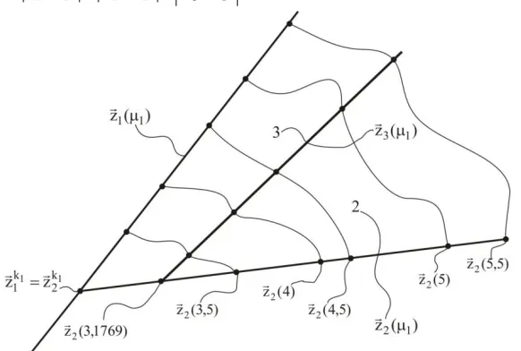
3. Example: As an example we give the following table of statistical data. Let the vectors
a
1
,
a
2
,
a
3
and the parameters k1
1
μ
and k22
μ have the following numerical values: a1=[1 1 1];
a2=[3 2 4, 5]; a3=[6 4 7]; m1k1=1.5 m2k2=2
The task of the investigation is to represent the points of the second piecewise-linear straight line depending on the first piecewise-linear vector-function
z
1(
1)
and unaccounted factors influence function
2(
2,
1,2) for arbitrary values of the parameter
1 changing in the interval μ 1,5 μ μ 8* 1 1 k
1
1 , in the form:
)]} ( 1 )[ ( 1 ){ ( )
( 1 1 1 1 2 1
2
z
A
z
Applying the above-stated numerical program to the given problem, we numerically define the points of the second piecewise-linear straight line
z
2(
1)
depending on the parameter
1
1
,
5
, that are represented in the form of the following table. It should be noted that the numerically constructed vectorsz
2(
1)
for different values of the parameter1
,
5
1
8
completely coincide with numerical results obtained earlier in the by developing theory of construction of piecewise-linear economic-mathematical models at uncertainty conditions in finite dimensional vector space stated in [1,2,7,13-15]. Below is a link to the table in the book [15]2.4. Algorithm of multi-variant computer modeling of prediction variables of economic event on the base of 2-component piecewise-linear economic-mathematical models in 3-dimensional vector space
In this section, based around the Matlab program, we suggest an algorithm and numerical programe for multi-variant prediction of economic event at uncertainty conditions on the vase of 2-component piecewise-linear model in 3-dimenaionl vector space.
) -( 2 1
1 1 1
1
1 a a a
zk
k )
)(
(
)
(
1 2 1 3 2 1 3 2 1 1 1 1 2 1 2a
a
z
a
z
a
k k k k k
) -( 2 11 1 1
2
2 a a a
zk
k )
(
)
(
)
)(
(
)
μ
-μ
(
z
1 1 1 1 2 1 2 1 3 2 1 3 1 2 1 3 1 k 1 1 k 2 k k k k kz
-a
z
-a
a
-a
z
-a
z
=
1 2 1 2 1 2 1 2 1 2 1 1 1 2 1 1 2 , 1 ) )( ( k k k k k k k k z z z z z z z zсos
) -( -) -( ) ( 1 1 1 1 1 1 2 1 1 1 1 2 1 2 1 2 a z z a z a a AA k k
k k k k
1 1 1 2 1 1 1 1 1 1 1 3 1 1 1 1 2 2 1 2-)
-(
)
-(
-)
(
1 1 2 1 2 2 1 1 2 2 1 2 2 2a
z
a
a
a
z
z
z
z
z
z
a
z
z
k k k k k k k k k k k k k k
2 , 1 2 2 , 1 2 2 2 2,
)
(
k
kсos
)]} ( 1 [ 1 { )
( 1 2 1 2 2 1,2
2
2 2
2 z =z +A +ω λ ,α
z
k k k) -( )
( 1 1 1 1 2 1
1 z a a a
z
2 1 3 1 2 1 3 1 1 2
)
(
)
)(
(
)
(
1 1 1 k k kz
a
a
a
z
a
) -( -) -( ) ( 1 1 1 1 1 1 2 1 1 1 1 1 1 a z z a z a a A k k k
1 1 1 2 1 1 1 1 1 1 1 3 1 1 1 1 2 1 2-)
-(
)
-(
-)
(
1 1 1 1 1 1a
z
a
a
a
z
z
z
z
z
z
a
z
z
k k k k kk
2 , 1 1 2 1 2 12 1 22(
(
),
)
(
)
(
)
сos)]} ( 1 )[ ( 1 { )
( 1 1 1 2 1
2
=z +A
+ω
z
) ) 1 ( ( ) ( ) 1
( 2 2
21 41 11 21 12 22 22 2 4 42 k k z a a a a a z a a
1
(
)
2(
1
2)
21 41 11 21 13 23 23 3 4 43 k k
![Table 5.2 (Below is a link to the table in the book [15])](https://thumb-us.123doks.com/thumbv2/123dok_us/8894966.1827320/17.612.143.469.571.751/table-link-table-book.webp)
![Table 5.3 (Below is a link to the table in the book [15])](https://thumb-us.123doks.com/thumbv2/123dok_us/8894966.1827320/19.612.141.469.69.598/table-link-table-book.webp)