Volume 55, 2018, Pages 68–80
GCAI-2018. 4th Global Con-ference on Artificial Intelligence
Historical Gradient Boosting Machine
Zeyu Feng
1, Chang Xu
1, and Dacheng Tao
1UBTECH Sydney AI Centre, The School of IT, FEIT, The University of Sydney, NSW, Australia
[email protected], {c.xu, dacheng.tao}@sydney.edu.au
Abstract
We introduce the Historical Gradient Boosting Machine with the objective of improving the convergence speed of gradient boosting. Our approach is analyzed from the perspective of numerical optimization in function space and considers gradients in previous steps, which have rarely been appreciated by traditional methods. To better exploit the guiding effect of historical gradient information, we incorporate both the accumulated previous gradients and the current gradient into the computation of descent direction in the function space. By fitting to the descent direction given by our algorithm, the weak learner could enjoy the advantages of historical gradients that mitigate the greediness of the steepest descent direction. Experimental results show that our approach improves the convergence speed of gradient boosting without significant decrease in accuracy.
1
Introduction
Gradient Boosted Decision Tree (GBDT) is one of the most popular machine learning algorithms and has been widely used in various modern machine learning and data mining applications. Taking decision tree of limited depth as weak learner (base learner), Gradient Boosting Ma-chine (GBM) [6] employs a gradient boosting scheme to produce a strong learner, and GBDT becomes an accurate, efficient and interpretable learning algorithm, which provides state-of-the-art results for a wide range of tasks, such as classification [14] and learning to rank [18,21,1]. By adapting to specific scenarios, it is shown to be effective to feature selection [22] and click through rate prediction [8]. Due to its high flexibility and remarkable performance, GBDT is also frequently used in data analytic competitions like Kaggle and KDDCup.
on the starting point of the optimization, Mohan et al. [18] improved GBRT to yield a better minimum point of high accuracy. However, this method (iGBRT) is much slower compared with both Random Forest (RF) and classical GBRT, since it needs the results of RF in advance as the initial guess. In recent years, several effective gradient boosted decision tree implemen-tations [3,10, 11] focused on the improvement of tree learner and contributed to the efficient tree construction and distributed computation, which makes them suitable for high dimensional and sparse data.
These aforementioned methods have greatly improved gradient boosting from different start-ing points. However, if analyzed from the perspective of numerical optimization in function space, all these methods aim to search in the steepest-descent direction to fit the weak tree learner. This steepest-descent step in gradient boosting is the greedy gradient direction calcu-lated with current prediction results to decrease the loss. However, beyond this greedy gradient direction, gradients of the objective function in previous steps also possess helpful information. These historical gradients usually represent the overall descent path of the optimization. The historical descent trend is beneficial for adjusting the current search direction and mitigat-ing the greedy effect of steepest descent gradient, as well as improvmitigat-ing the convergence speed as a result. However, in the context of gradient boosting, such information has rarely been appreciated and exploited for a better descent step.
In this paper, we present a historical gradient boosting algorithm that takes account of historical gradients to improve the optimization of GBM. If small steps continuously indicate the same direction, we could amplify the effects and accelerate the learning speed. Specifically, we incorporate gradient values from both previous accumulated steps and current step into the computation of descent direction in function space. We develop two strategies to utilize historical gradients, adding historical gradients to the current steepest direction or to a gradi-ent estimated at an updated location. These strategies are consistgradi-ent with the general idea of accelerated gradient descent methods momentum and nesterov in numerical optimization, and thus we inherit their advantages, e.g. accelerating convergence and dampening oscillations. Be-yond the current local gradient, the weak learner in each iteration can also observe the helpful descent trends we have experienced in past updates. To reduce the number of instances in train-ing, the proposed historical gradient boosting is then extended into the stochastic optimization scenario. Two different techniques are developed to handle examples that do not participated in last update and have no historical gradient. Experimental results on four publicly available datasets demonstrate the effectiveness of the proposed approach in improving the convergence speed and hence reducing training time of GBDT while without significant decrease in accuracy.
2
Gradient Boosted Decision Tree
In this section we review GBDT method from the perspective of numerical optimization in function space.
2.1
Tree Ensemble Model
For a given training sample with N observations D = {(xi, yi)}N1, where xi ∈ X ⊆ Rp and
yi ∈ Y ⊆R, our goal is to construct a predictor F :X → Y, which has an additive expansion
of the form
F(x) =
M
X
m=1
where h: X → R is usually a simple parameterized weak (base) learner chosen in a class of functionsH. To learn the set of functions, we minimize the following empirical risk function
L=
N
X
i=1
l(yi, M
X
m=1
βmhm(xi)) (2)
over the linear combinations of functions inH. Herel(·,·) is a differentiable convex loss function that measures the difference between the predictionF(xi) and the labelyi.
For tree ensemble model, the base learner is chosen as regression tree
h(x;{bj, Rj}J1) =
J
X
j=1
bj1(x∈Rj), (3)
where J is the number of terminal nodes in regression tree. {Rj}J1 represents each region of
the tree that maps an example to the corresponding leaf and {bj}J1 is the value on each leaf.
We can express predictorF(x) as an additive of regression trees
F(x) =
M
X
m=1
βm J
X
j=1
bjm1(x∈Rjm). (4)
To simplify notation, we alternatively express the weak learner as fm(x) = PJj=1γjm1(x ∈
Rjm) by combining the coefficients, i.e. γjm=βmbjm. In order to solve Eq. (2), we can adopt
a greedy stagewise approach that requires the model to be trained in an additive manner. The weak tree learner at them-th iteration can be obtained via minimizing the following objective
L(f) =
N
X
i=1
l(yi, Fm−1(xi) +f(xi)), (5)
and
fm(x) = arg min f
L(f). (6)
For each iteration, computation of the minimization requires the prediction results of the current committee. Then the model is updated as follows
Fm(x) =Fm−1(x) +fm(x). (7)
To reduce overfitting, typically a shrinkage term (learning rate)is added on the newly fitted treefm(x) in computing the model update for the current iteration. In most of the time, the
learning rate is usually fixed to be a small constant number less than 0.1, which could alleviate overfitting.
2.2
Greedy Gradient Descent
In the context of gradient boosting, the weak tree learner in each iteration is constructed to fit the negative gradient direction−gm={−gm(xi)}N1 evaluated atFm−1(x) in theN-dimensional
data space by least-squares
fm= arg min f
N
X
i=1
where −gm(xi) = −[
∂l(yi,F(xi))
∂F(xi) ]F(x)=Fm−1(x). This step is an approximation to −gm in tree spaceHandgmis regarded as the steepest descent direction. The optimal weight for each leaf of the tree is computed by line search
γjm= arg min γ
X
xi∈Rjm
l(yi, Fm−1(xi) +γ). (9)
Another popular strategy to optimize the additive objective comes from second order Taylor expansion of Eq. (5) [5]. Using regression tree as weak learner, minimization of the loss is derived as follows [3]
min
f L(f)
≈min
f N
X
i=1
[l(yi, Fm−1(xi)) +gm(xi)f(xi) +
1
2hm(xi)f(xi)
2]
= min
f N
X
i=1
[gm(xi)f(xi) +
1
2hm(xi)f(xi)
2]
= min
γ J
X
j=1
[ (X
i∈Ij
gm(xi))γj+
1 2(
X
i∈Ij
hm(xi))γj2],
(10)
where hm(xi) = [ ∂2l(y
i,F(xi))
∂F(xi)2 ]F(x)=Fm−1(x). The optimal weight for each leaf can be easily obtained as
γjm=−
P
xi∈Rjmgm(xi) P
xi∈Rjmhm(xi)
. (11)
The greedy gradient descent and second-order approximation of Eq. (5) described in this section are based on numerical optimization in function space, in which the base learner acts as variables to be optimized.
3
Historical Gradient Boosting
In the classical gradient boosting methods described in the previous section, only current deriva-tive and curvature information are taken into consideration, which yield a greedy step. We make an observation that historical gradient information could also be exploited for gradients update in gradient boosting. Given these historical gradients, we hope to improve the convergence speed, and hence reduce training time.
3.1
Historical Gradient Descent
During each function update step of gradient boosting, only a small distance is actually moved toward the steepest descent direction on the loss surface. To accelerate this process, we consider the gradient values from previous update steps by exploiting both current and historical first-order information. Motivated by this, we propose computing the descent direction by using the combination of these two gradients as the pseudo responses for the followed least-squares fitting. Particularly, two strategies are examined.
−gmbe the steepest descent gradient on discrete data atm-th iteration, and itsi-th component is defined as−gm(xi) =−[
∂l(yi,F(xi))
∂F(xi) ]F(x)=Fm−1(x). In each step, we aim to provide an alterna-tive descent direction vector vm. For previously calculated vector vm−1, we multiply a decay
coefficient and then combine this term with the current negative gradient. This term records past gradient values and forces the update to move under the influence of previous directions. Therefore, we give the descent direction vectorvmcalculated recursively as
vm=µvm−1−gm, (12)
where is the learning rate and µ∈[0,1] is the coefficient for accumulated gradients. In our methods, the weak tree learner aims at fitting this descent direction vectorvmrather than the
negative gradient−gmestimated with the current prediction results. The least-square Problem
(8) then becomes
fm= arg min f
N
X
i=1
[vmi−f(xi)]2, (13)
wherevmi is thei-th coordinate of the vectorvm. The newly fitted weak tree is added to the
current committee with the leaf value being set to the mean value of allvmi that are divided
into each node.
To summarize, the pseudo-code implementation of our historical GBM via previous gradient accumulation is
Algorithm 1Historical GBM – Momentum
Require: Learning rate, accumulated gradient coefficient µ, iteration numberM Input: Training sampleD={(xi, yi)}N1
Output: Additive tree ensembleFm 1: InitializationF0(x),v0,m= 1
2: while m≤M do
3: −gm(xi) =−[
∂l(yi,F(xi))
∂F(xi) ]F(x)=Fm−1(x), i= 1, ..., N
4: vm=µvm−1−gm
5: {Rjm}J1 =J-terminal node tree({(vmi,xi)}N1)
6: γjm=|R1jm|Pxi∈Rjmvmi, j= 1, ..., J 7: Fm(x) =Fm−1(x) +P
J
j=1γjm1(x∈Rjm)
8: m=m+ 1
9: end while
The main difference of our approach from classical gradient boosting lies in this descent direction calculation. For squared-error loss function, the proposed algorithm falls back to the original algorithm when the coefficientµfor accumulated gradients is set to zero.
Historical GBM – Nesterov: Our descent direction calculation is actually consistent with the idea of momentum method in numerical optimization [20]. We also notice that an-other accelerated gradient method nesterov is effective and also has faster convergence speed in numerical optimization. Nesterov’s accelerated gradient (NAG) [19] has a close relation to classical momentum. In a similar fashion, we could consider computing gradient at a location F(x) =Fm−1(x) + ˜fm(x) where the previous descent step continue to update the current
com-mittee. f˜m(x) is fitted to the accumulated directionvm−1. However, this simple update in
form in replace of ˜fm(x), and the corresponding computation of step 4 in algorithm1have the
following form
−˜gm(xi) =−[
∂l(yi, F(xi))
∂F(xi)
]F(x)=Fm−1(x)+µvm−1 (14)
vm=µvm−1−˜gm, (15)
where ˜gm is the gradient vector estimated at a location where a minor step is added along the previous descent direction.
It would be better to compare our algorithm with classical gradient boosting machine through theoretical analysis. But it is difficult to obtain the theoretical convergence rate of our historical GBM. And to our knowledge, there is currently no proof of convergence rate of classical GBM either. However, we do observe the fact that the accumulated historical gradients are beneficial for descent direction searching. When successive steps continuously indicate same direction, small step updates could be amplified. On the other hand, when gradients are os-cillating fast, accumulated historical term could dampen this behavior. Both these will impact a positive influence on convergence. Furthermore, the effect of improvement on convergence speed is also demonstrated by our empirical experiments.
3.2
Historical Stochastic GBDT
Friedman [7] developed a stochastic version of gradient boosting, in which at each iteration only a randomly selected subsample of the training date is used to fit the weak learner. The ad-vantages are twofold, less computational time and higher variance reduction. In the meantime, introducing random sampling will bring noises to the learning problem. When the weak tree learner is greedily fitted to the current gradient of a mini-batch sample, it cannot guarantee the prediction quality for instances outside the mini-batch.
As a straightforward extension of historical gradient boosting, we incorporate accumulated gradients into stochastic gradient boosting. By taking a random permutation{π(i)}N
1 of
inte-gers{1, ..., N} at each iteration, we calculate descent direction on a subsample data{xπ(i)} ˜
N
1
with size ˜N < N. Since the functional derivative is executed in data space in gradient boosting, the two subsample{xπm−1(i)}
˜
N
1 and{xπm(i)}
˜
N
1 in successive iterations may or may not overlap.
As a result, some instances in the current subsample will not have previous gradient values. We use two ways to tackle this problem.
Full Gradient Update: The first way we use is to compute the gradient values for all data points at each round, which is same as Eq. (12). Then the weak tree learner is fitted to the updated descent direction in subsample
fm= arg min f
˜
N
X
i=1
[vmπ(i)−f(xπ(i))]2. (16)
This ensures that each example maintains gradient information no matter whether it is in the subsample or not and will actually bring extra computational burden to original SGB. But compared with the time complexity of tree construction (O(N ×p) for pre-sorted algorithm, where p represents the number of features), this (with a time complexity of O(N)) will not increase the total computational time significantly. Take the momentum-like historical gradient boosting for example, the pseudo code of its extension on SGB is summarized in algorithm2.
Algorithm 2Historical Stochastic GBM – Momentum
Require: Learning rate, accumulated gradient coefficientµ, iteration numberM, subsample size ˜N
Input: Training sampleD={(xi, yi)}N1
Output: Additive tree ensembleFm 1: InitializationF0(x),v0,m= 1
2: while m≤M do
3: {π(i)}N
1 = random permutation{i}N1
4: −gm(xi) =−[
∂l(yi,F(xi))
∂F(xi) ]F(x)=Fm−1(x), i= 1, ..., N
5: vm=µvm−1−gm
6: {Rjm}J1 =J-terminal node tree({(vmπ(i),xπ(i))} ˜
N
1 )
7: γjm=|R1jm| P
xπ(i)∈Rjmvmπ(i), j= 1, ..., J
8: Fm(x) =Fm−1(x) +P
J
j=1γjm1(x∈Rjm)
9: m=m+ 1
10: end while
of historical gradients are defined within one iteration. At the m-th iteration, for an instance xπm(i)∈ {xπm−1(j)}
˜
N
1 ∩ {xπm(j)}
˜
N
1, its descent direction is computed via
vmπm(i)=µv(m−1)πm(i)−gm(xπm(i)).
If this instance does not belong to the previous subsample, i.e. xπm(i)∈ {xπm(i)}
˜
N
1 \{xπm−1(i)}
˜
N
1,
its descent direction value is simply set as the current gradient multiplied with the learning rate
vmπm(i)=−gm(xπm(i)). We will compare the results of these two ways in Section4.2.
4
Experimental Results
In this section we report the empirical evaluation results of our algorithm. We first compare the overall number of iterations needed as well as the test accuracy of our two historical GBM algo-rithms against the classical GBM with line search and GBM with second order approximation on various datasets, which could represent the convergence speed and test performance, respec-tively. The difference between full and partial gradient update strategy in historical stochastic GBDT scenario is then compared and analyzed. We study the sensitivity of historical coefficient at the end of this section.
4.1
Dataset and Experimental Setup
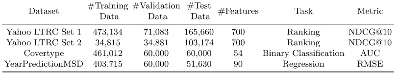
We use four publicly available datasets in our experiments, which have been widely used to evaluate gradient boosting methods. Table1summarized the detailed statistics of all datasets. The first two datasets we used are from Yahoo! Inc.’s Learning to Rank Challenge (LTRC) [2]. These are typical datasets for learning to rank problems and contain both dense and sparse features. We use the predefined training, validation and test split setting in our experiment.
The other two datasets come from the UCI Machine Learning Repository [15]. We randomly select approximately 80% of the samples in Covertype1for training and the remaining 20% are
Dataset #Training #Validation #Test #Features Task Metric
Data Data Data
Yahoo LTRC Set 1 473,134 71,083 165,660 700 Ranking NDCG@10 Yahoo LTRC Set 2 34,815 34,881 103,174 700 Ranking NDCG@10
Covertype 461,012 60,000 60,000 54 Binary Classification AUC YearPredictionMSD 403,715 60,000 51,630 90 Regression RMSE
Table 1: Dataset information used in experiments.
evenly divided into validation and test set. The official train/test split suggestion is followed for YearPredictionMSD2 (Abbreviated as MSD in the following text) dataset. We take about
1/8 examples in training set for validation purpose.
We learn the weak tree greedily layer by layer and the implementation is based on the open source code pGBRT [21], which implements a plain GBRT algorithm. Our algorithm could be further accelerated by using more efficient tree construction methods or distributed learning proposed by several recent implementations like XGBoost and LightGBM. These solvers accel-erate the tree construction algorithm by approximating or sampling the gradients. In contrast, the main purpose of this paper is to study the effect of historical gradients. Therefore for a fair comparison, all comparisons in our experiments are based on this plain GBDT, which implements a vanilla tree construction without affecting gradient values.
Following the settings used in [18, 21], each weak regression tree learner is set to have a maximum depth equals 4 and the learning rate of gradient boosting is set to 0.06. Here we mainly focus on evaluating the effect of historical gradient and hence keep the learning rate fixed. Our approach can be generalized to handle adaptive learning rate strategies as AdaGrad [4] and Adam [12] by modifying the gradient update formula of Eq. (12). The performance of binary classification, ranking and regression are measured in AUC, NDCG@10 [9] and RMSE, respectively. For all experiments, we set the maximum number of trees (iterations) to be 6000 and use early stopping to terminate training. Training process will end if the metric values on corresponding validation sets do not improve after a fixed number of training iterations. Through the parameter analysis in Section4.3, we found that historical coefficientµbelow 0.5 could achieve stable results and hence we set this to 0.5 for illustration. The sampling rate for stochastic GBM is set to 0.2.
4.2
Evaluation Results
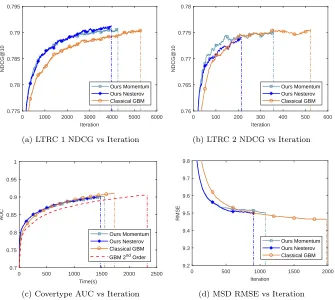
Figure1illustrates the accuracy-iteration curves of the four GBM algorithms on four test sets. The vertical dashed lines represent the iteration that triggers early stopping. The overall number of iterations and running time are also summarized in Table 2. In ranking problem we use a pointwise squared-loss in the optimization, which is same as the loss function used in regression. Since under this objective, classical GBM with line-search and second order approximation method will lead to exact same outcome, here we report them as one result. As expected, under the same hyper-parameter setting, our two methods need fewer iterations to achieve convergence compared with classical GBM and hence effectively improve the convergence speed. Total running times are also reduced as a consequence. Specifically, in ranking and regression task, both historical GBM momentum and nesterov have a faster convergence speed than classical GBM method. For classification task, the early stopping criteria is not triggered. We hence
0 1000 2000 3000 4000 5000 6000 Iteration
0.775 0.78 0.785 0.79 0.795
NDCG@10
Ours Momentum Ours Nesterov Classical GBM
(a) LTRC 1 NDCG vs Iteration
0 100 200 300 400 500 600 Iteration
0.76 0.765 0.77 0.775 0.78
NDCG@10
Ours Momentum Ours Nesterov Classical GBM
(b) LTRC 2 NDCG vs Iteration
0 500 1000 1500 2000 2500 Time(s)
0.7 0.75 0.8 0.85 0.9 0.95 1
AUC
Ours Momentum Ours Nesterov Classical GBM GBM 2nd Order
(c) Covertype AUC vs Iteration
0 500 1000 1500 2000 Iteration
9.2 9.3 9.4 9.5 9.6 9.7 9.8
RMSE
Ours Momentum Ours Nesterov Classical GBM
(d) MSD RMSE vs Iteration
Figure 1: Accuracy-iteration results of different GBM methods in non-stochastic scenario on four datasets. The vertical dashed lines represent the early stopping step for each method. Accuracy-time result is reported for Covertype dataset.
Dataset Ours Momentum Ours Nesterov Classical GBM GBM 2ndOrder
LTRC 1 #Iter(Time) 4,261(1.3×10⁴) 3,964(1.2×10⁴) 5,280(1.8×10⁴) – LTRC 2 #Iter(Time) 358(0.8×10²) 214(0.5×10²) 523(1.1×10²) – Covertype #Iter(Time) 6,000(1.5×10³) 6,000(1.4×10³) 6,000(1.7×10³) 6,000(2.3×10³)
MSD #Iter(Time) 2,812(3.2×10³) 3,663(4.1×10³) 4,732(5.2×10³) –
Table 2: The number of total iterations in training and the corresponding CPU time (seconds) for non-stochastic GBM.
compare the results with respect to the running time. We can see that historical GBM has a faster trend to convergence point. It also shows that our method has a smaller time complexity. The final test accuracy are summarized in table3. We can see that our two historical GBM methods can achieve comparable test accuracy with baseline GBM methods.
ac-Dataset Metric Ours Momentum Ours Nesterov Classical GBM GBM 2nd Order
LTRC 1 NDCG@10 0.7909 0.7913 0.7905 –
LTRC 2 NDCG@10 0.7757 0.7741 0.7756 –
Covertype AUC 0.9018 0.9018 0.9105 0.9058
MSD RMSE 9.3984 9.3883 9.3924 –
Table 3: Final accuracy on test set for non-stochastic GBM.
0 500 1000 1500 2000 2500 Iteration
0.74 0.75 0.76 0.77 0.78 0.79 0.8
NDCG@10
Ours Momentum Ours Nesterov Classical GBM
(a) LTRC 1 NDCG vs Iteration
0 50 100 150 200 250 300 350 Iteration
0.72 0.73 0.74 0.75 0.76 0.77 0.78
NDCG@10
Ours Momentum Ours Nesterov Classical GBM
(b) LTRC 2 NDCG vs Iteration
0 500 1000 1500 2000 2500 Time(s)
0.7 0.75 0.8 0.85 0.9 0.95 1
AUC
Ours Momentum Ours Nesterov Classical GBM GBM 2nd Order
(c) Covertype AUC vs Iteration
0 1000 2000 3000 4000 5000 Iteration
9.2 9.3 9.4 9.5 9.6 9.7 9.8
RMSE
Ours Momentum Ours Nesterov Classical GBM
(d) MSD RMSE vs Iteration
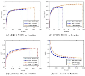
Figure 2: Accuracy-iteration results of different stochastic GBM methods with full gradient update on four datasets. The vertical dashed lines represent the early stopping step for each method. Accuracy-time result is reported for Covertype dataset.
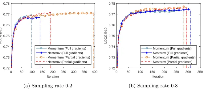
curacy decrease than that in non-stochastic scenario. Two historical gradient update strategies are compared in Figure 3. We observed that for large sampling rate, the two methods differ less. For a small sampling rate, calculating historical gradients for every instance could have a large influence on the convergence speed.
4.3
Analysis on Historical Gradient Parameter
Dataset Ours Momentum Ours Nesterov Classical GBM GBM 2ndOrder
LTRC 1 #Iter(Time) 1,076(3.7×10³) 1,599(5.3×10³) 2,077(7.1×10³) – LTRC 2 #Iter(Time) 98(2.1×101) 138(3.1×101) 338(7.6×101) – Covertype #Iter(Time) 6,000(1.8×10³) 6,000(1.7×10³) 6,000(1.9×10³) 6,000(2.3×10³)
MSD #Iter(Time) 1,082(5.8×10²) 906(4.7×10²) 1,979(1.1×10³) –
Table 4: The number of total iterations in training and the corresponding CPU time (seconds) for stochastic GBM.
Dataset Metric Ours Momentum Ours Nesterov Classical GBM GBM 2nd Order
LTRC 1 NDCG@10 0.7828 0.7834 0.7865 –
LTRC 2 NDCG@10 0.7702 0.7673 0.7752 –
Covertype AUC 0.9164 0.9160 0.9121 0.9129
MSD RMSE 9.5012 9.4997 9.4627 –
Table 5: Final accuracy on test set for stochastic GBM.
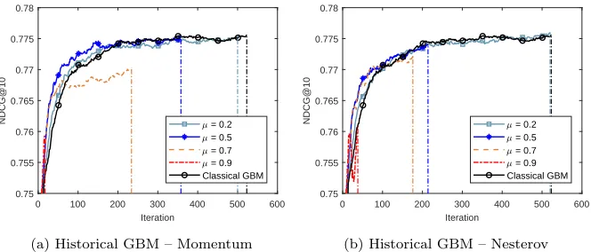
LTRC set 2 behaves as a function of the total iterations needed under different historical coef-ficients. We observed that the improvement on test results becomes stable when the coefficient is set to a value below 0.5.
5
Conclusion
In this paper, we propose historical GBM by considering cumulated previous gradients, which have the ability to alleviate the greediness of steepest-descent gradient and accelerate conver-gence speed. We also extend historical GBM to stochastic scenario and compare full gradient update with partial gradient update under different sampling rate. The historical coefficient µ is analyzed and we suggest that a value lower than 0.5 could yield a stable results. We compare our two historical GBM methods against classical GBM with line search and second
0 50 100 150 200 250 300 350 400 Iteration
0.72 0.73 0.74 0.75 0.76 0.77 0.78
NDCG@10
Momentum (Full gradients) Nesterov (Full gradients) Momentum (Partial gradients) Nesterov (Partial gradients)
(a) Sampling rate 0.2
0 50 100 150 200 250 300 350 Iteration
0.72 0.73 0.74 0.75 0.76 0.77 0.78
NDCG@10
Momentum (Full gradients) Nesterov (Full gradients) Momentum (Partial gradients) Nesterov (Partial gradients)
(b) Sampling rate 0.8
0 100 200 300 400 500 600 Iteration
0.75 0.755 0.76 0.765 0.77 0.775 0.78
NDCG@10 = 0.2
= 0.5 = 0.7 = 0.9 Classical GBM
(a) Historical GBM – Momentum
0 100 200 300 400 500 600 Iteration
0.75 0.755 0.76 0.765 0.77 0.775 0.78
NDCG@10 = 0.2
= 0.5 = 0.7 = 0.9 Classical GBM
(b) Historical GBM – Nesterov
Figure 4: Accuracy-iteration results of two historical GBM methods under various coefficient µon LTRC set 2.
order approximation through experiments on public datasets. It shows that with same learning parameters, our approach outperforms plain GBM in terms of convergence speed and training time, and achieves an average speed-up about 50% on four datasets. More speed-up can be expected if considering state-of-the-art tree learners.
References
[1] Chris J.C. Burges. From RankNet to LambdaRank to LambdaMART: an overview. Technical report, June 2010.
[2] Olivier Chapelle and Yi Chang. Yahoo! learning to rank challenge overview. InProceedings of the Learning to Rank Challenge, volume 14 ofProceedings of Machine Learning Research, pages 1–24, Haifa, Israel, June 2011. PMLR.
[3] Tianqi Chen and Carlos Guestrin. XGBoost: a scalable tree boosting system. InProceedings of the 22nd ACM SIGKDD International Conference on Knowledge Discovery and Data Mining, pages 785–794. ACM, 2016.
[4] John Duchi, Elad Hazan, and Yoram Singer. Adaptive subgradient methods for online learning and stochastic optimization.Journal of Machine Learning Research, 12:2121–2159, 2011. [5] Jerome Friedman, Trevor Hastie, and Robert Tibshirani. Additive logistic regression: a statistical
view of boosting (with discussion and a rejoinder by the authors). The Annals of Statistics, 28(2):337–407, April 2000.
[6] Jerome H. Friedman. Greedy function approximation: a gradient boosting machine. The Annals of Statistics, 29(5):1189–1232, 2001.
[7] Jerome H. Friedman. Stochastic gradient boosting. Computational Statistics & Data Analysis, 38(4):367–378, 2002.
[8] Xinran He, Junfeng Pan, Ou Jin, Tianbing Xu, Bo Liu, Tao Xu, Yanxin Shi, Antoine Atallah, Ralf Herbrich, Stuart Bowers, and Joaquin Qui˜nonero Candela. Practical lessons from predicting clicks on ads at facebook. InProceedings of the Eighth International Workshop on Data Mining for Online Advertising, ADKDD’14, pages 5:1–5:9, New York, NY, USA, 2014. ACM.
[9] Kalervo J¨arvelin and Jaana Kek¨al¨ainen. Cumulated gain-based evaluation of IR techniques.ACM Transactions on Information Systems, 20(4):422–446, 2002.
281–284, April 2017.
[11] Guolin Ke, Qi Meng, Thomas Finley, Taifeng Wang, Wei Chen, Weidong Ma, Qiwei Ye, and Tie-Yan Liu. LightGBM: a highly efficient gradient boosting decision tree. In Advances in Neural Information Processing Systems 30, pages 3149–3157. Curran Associates, Inc., 2017.
[12] Diederik P. Kingma and Jimmy Ba. Adam: A method for stochastic optimization. InThe 3rd International Conference on Learning Representations, San Diego, CA, USA, 2015.
[13] Ling Li, Yaser S. Abu-Mostafa, and Amrit Pratap. CGBoost: conjugate gradient in function space. Caltech Computer Science Technical Report CaltechCSTR:2003.007, Calfornia Institute of Technology, 2003.
[14] Ping Li. Robust logitboost and adaptive base class (ABC) logitboost. In Proceedings of the Twenty-Sixth Conference on Uncertainty in Artificial Intelligence, UAI’10, pages 302–311, Arling-ton, Virginia, United States, 2010. AUAI Press.
[15] Moshe Lichman. UCI machine learning repository, 2013.
[16] Llew Mason, Jonathan Baxter, Peter Bartlett, and Marcus Frean. Boosting algorithms as gradient descent. InProceedings of the 12th International Conference on Neural Information Processing Systems, NIPS’99, pages 512–518, Cambridge, MA, USA, 1999. MIT Press.
[17] Llew Mason, Jonathan Baxter, Peter Bartlett, and Marcus Frean. Functional gradient techniques for combining hypotheses. InAdvances in Large Margin Classifiers, pages 221–246. MIT Press, Cambridge USA, 2000.
[18] Ananth Mohan, Zheng Chen, and Kilian Weinberger. Web-search ranking with initialized gra-dient boosted regression trees. InProceedings of the Learning to Rank Challenge, volume 14 of Proceedings of Machine Learning Research, pages 77–89, Haifa, Israel, June 2011. PMLR. [19] Yurii Nesterov. A method of solving a convex programming problem with convergence rate
O(1/K2). Soviet Mathematics Doklady, 27(2):372–376, 1983.
[20] B.T. Polyak. Some methods of speeding up the convergence of iteration methods. USSR Compu-tational Mathematics and Mathematical Physics, 4(5):1 – 17, 1964.
[21] Stephen Tyree, Kilian Q. Weinberger, Kunal Agrawal, and Jennifer Paykin. Parallel boosted regression trees for web search ranking. InProceedings of the 20th International Conference on World Wide Web, WWW ’11, pages 387–396, New York, NY, USA, 2011. ACM.
[22] Zhixiang Xu, Gao Huang, Kilian Q. Weinberger, and Alice X. Zheng. Gradient boosted fea-ture selection. InProceedings of the 20th ACM SIGKDD International Conference on Knowledge Discovery and Data Mining, KDD ’14, pages 522–531, New York, NY, USA, 2014. ACM. [23] Zhaohui Zheng, Hongyuan Zha, Tong Zhang, Olivier Chapelle, Keke Chen, and Gordon Sun. A