Free boundary value problems and hjb equations for the stochastic optimal control of elasto-plastic oscillators

B. Bouchard, J.-F. Chassagneux, F. Delarue, E. Gobet and J. Lelong, Editors

FREE BOUNDARY VALUE PROBLEMS AND HJB EQUATIONS FOR THE

STOCHASTIC OPTIMAL CONTROL OF ELASTO-PLASTIC OSCILLATORS

M. Lauriere

_{, Z. Li}

_{, L. Mertz}

_{, J. Wylie}

_{and S. Zuo}

Abstract. We consider the optimal stopping and optimal control problems related to stochastic vari-ational inequalities modeling elasto-plastic oscillators subject to random forcing. We formally derive the corresponding free boundary value problems and Hamilton-Jacobi-Bellman equations which belong to a class of nonlinear partial of differential equations with nonlocal Dirichlet boundary conditions. Then, we focus on solving numerically these equations by employing a combination of Howard’s al-gorithm and the numerical approach [A backward Kolmogorov equation approach to compute means, moments and correlations of non-smooth stochastic dynamical systems; Mertz, Stadler, Wylie; 2017] for this type of boundary conditions. Numerical experiments are given.

R´esum´e. Nous consid´erons les probl`emes de l’arrˆet optimal et du contrˆole optimal associ´es `a des in´equations variationelles stochastiques mod´elisant des oscillateurs ´elasto-plastiques sous for¸cage al´ea-toire. Nous obtenons formellement les probl`emes `a fronti`ere libre et les ´equations de Hamilton-Jacobi-Bellman correspondantes qui appartiennent `a une classe d’´equations aux d´eriv´ees partielles nonlin´eaires avec des conditions aux bord de Dirichlet nonlocales. Ensuite, nous nous concentrons sur la r´esolution num´erique de ces ´equations en employant une combinaison de l’algorithme d’Howard et de l’approche num´erique [A backward Kolmogorov equation approach to compute means, moments and correlations of non-smooth stochastic dynamical systems; Mertz, Stadler, Wylie; 2017] pour ce type de conditions aux bord. Des exp´eriences num´eriques sont pr´esent´ees.

1.

_{Motivations and background}

In an extremely wide range of applications, mechanical systems are fundamentally affected by vibrations. For instance, components (such as pipes) in a power plant are designed to be structurally robust under seismic vibrations. Vibrations also cause mechanical systems to accumulate plastic deformations and eventually fail. The importance of these issues has motivated a lot of effort in modeling. From the modeling point of view, keeping track of the impact of past vibrations requires a specific description of the mechanical systems under consideration. The state of the system must be described by a randomly forced dynamical system with memory. Random forcing here expresses the stochastic nature of the vibrations that apply to the mechanical structures. In this framework, the difficulty is to handle dynamical systems with memory. A huge engineering literature has been devoted to this topic [14,17,18,25,29,31,34–36,40,41]. This paper mainly focuses on an important model, referred to as the elastic-perfectly-plastic oscillator (EPPO), which was introduced in [28] and appears

1

ORFE, Princeton University, Princeton, NJ 08540, USA; e-mail:[email protected]

2

ECNU-NYU Institute of Mathematical Sciences, NYU Shanghai, Shanghai, China; e-mail:[email protected], e-mail: [email protected], e-mail: [email protected]

3

Department of Mathematics, City University of Hong Kong, Hong Kong, China; e-mail:[email protected]

c

EDP Sciences, SMAI 2019 This is an Open Access article distributed under the terms of the Creative Commons Attribution License (http://creativecommons.org/licenses/by/4.0),

which permits unrestricted use, distribution, and reproduction in any medium, provided the original work is properly cited.

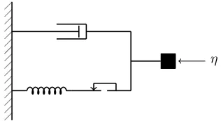
in various applications [16,19–21,23,24]. In terms of rheology, the response of such model is a combinations of elementary rheological models : springs, Saint-Venant’s elements, dashpots and material points as shown in Figure1.

η

Figure 1. Rheological model of an elasto-perfectly-plastic oscillator. A mass (black box) is associated in series with elements which are themselves an association in parallel or in series of elementary rheological models. The whole system is excited by a time-dependent forceη.

In [12,13], the stochastic variational inequalities (SVIs) have been identified as the right mathematical tool to deal with this model. Here, our objective is to derive and solve numerically a new class of free boundary problems and Hamilton-Jacobi-Bellman equations related to the control of these SVIs. Below, we provide background on and identify research issues on a stochastically driven EPPO.

1.1.

An elasto-perfectly-plastic problem with noise

The dynamics focuses on two quantities: the deformation supported by the structure, namelyxt, when subjected to the vibrations, and its velocity, namelyyt“x9t. In the simplest case, the dynamics of the velocity is given by

9

yt`c0yt`ft“ηt, wherec0ą0 is a damping coefficient,ηtdescribes the random vibrations and ftdescribes the restoring force arising from the structure. The exact nature offtdepends on the particular structure under consideration. The so-called perfect model corresponds to the case in which the forceft is a linear function of

xt in the elastic phase and a constant in the plastic phase. In this case, the permanent (plastic) deformation at time t can be written as ∆t fi ş

t

01t|fs|“kYuysds, where kY describes the plastic phase through a stiffness

coefficient k and an elasto-plastic bound, that is normalized to Y “1. The variable zt “xt´∆t describes the deformation without plastic deformation. When |zt| ă1, the structure is in the elastic regime and when

|zt| “1, it is in the plastic regime. In both cases, the restoring forceft is given bykzt. The dynamics is then described by the pair pyt, ztqthat satisfies

9

yt`c0yt`kzt“ηt, pz9t´ytqpφ´ztq ě0, @|φ| ď1, |zt| ď1,@t. (1)

1.2.

Research Issues

From a mathematical perspective, the point is to understand the behavior of the model in order to predict the behavior of the mechanical structure of interest. For engineering applications, this is fundamental in assessing the risk of failure of the structure. In [5,6,12], the ergodic behavior of the couple velocity-restoring force pyt, ztqof an elasto-perfectly-plastic oscillator (EPPO) excited by white noise and by a filtered noise has been established. The invariant probability can be described, through its density, as the solution of a partial differential equation (PDE), with specific boundary conditions arising from the plastic properties of the model. It is worth mentioning that ergodicity does not hold for the plastic deformation ∆t. Thus, the behavior of ∆t can be investigated through different quantities such as

(growth rate) variance of the plastic deformation E

“

∆2

T

‰

T and the failure risk P

ˆ

max

0ďtďT|∆t| ěb

˙

wherebis a critical threshold of deformation considered as dangerous for the system andp0, Tqis a given interval of time. For large time, analysis of the variance for the plastic deformation (2) has been carried out in [8] for an EPPO excited by white noise and a probabilistic formula has been derived. Also, in [7] an analytical formula has been proven. Concerning the failure risk, the mathematical techniques that have been developed so far provide an asymptotic formula [30]. Analysis of the risk raises other important problems for which no answer has been given so far.

‚ The risk probability (2) can be reformulated in terms of an optimal stopping problem as follows:

sup τPT0,T

Pp|∆τ| ěbq, where T0,T is the set of stopping timeτ in the intervalr0, Ts.

This reformulation relies on a general result on reachability for Markov processes [10]. The problem is technically delicate1

. Here, we rather focus on a similar problem for the plastic state, that is,

sup τPT0,T

Pp|zτ| “1q “PpDtP r0, Ts,|zt| “1q. (3)

Insubsection 2.1, we describe a general framework based on a new class of free boundary value problems characterizing optimal stopping problems of the form

sup τPT0,T

E

ˆżτ

0

e´λsgpzs, ysqds`e´λτfpzτ, yτq

˙

.

‚ Another important concept related to the notion of critical excitation [38] must be considered. The major point is to answer the following question: can we find the most likely random force, of the form ηt“αt`w9twhere wt is a Wiener process, that would maximize the accumulation of the plastic deformation or the time spent in plastic regime or in the sense

sup αp.qE

˜ żT

0

1t|zs|“1u|ys|ds ¸

or sup αp.qE

˜ żT

0

1t|zs|“1uds ¸

. (4)

We aim at translating the problem within the framework of stochastic control. In subsection 2.2, we describe a general framework based on a new class of Hamilton-Jacobi-Bellman Equations aimed at characterizing the controlαin the form

sup αp.qE

˜ żT

0

e´λsgpzs, ysqds`fpzT, yTq

¸

.

1.3.

Notations

GivenT ą0, setDT fip´1,1q ˆRˆ r0, Ts,D_T`fit1u ˆRˆ r0, TsandD<sub>T</sub>´fit´1u ˆRˆ r0, Ts. Then, define three differential operatorsA,B` andB´ as follows

Afi1₂ B

2

By2 ´ pc0y`kzq B By `y

B

Bz and B˘ fi

1 2

B2

By2 ´ pc0y˘kq B

By ˘minp0,˘yq

B Bz.

We use the notation C_T‹ for the set of continuous functions on r´1,1s ˆRˆ r0, Ts that are C1_{-regular with}

respect to z,C2_{-regular with respect to}

y andC1_{-regular with respect to}

t.

1

In order to treat the optimal stopping problem related to (2), we would need to extend the state variable from pzt, ytq to

pzt, yt, xtq(orpzt, yt,∆tq) and thus leading to a three dimensional free boundary value problem. From a computational viewpoint,

1.4.

Overview of our numerical study

The PDEs related to the optimal stopping and optimal stochastic control of the elasto-plastic oscillator are non-standard free boundary value and HJB problems. To the best of our knowledge, it seems they have not been treated in the literature. In the linear case that is without control (i.e backward Kolmogorov equations), only partial existence and uniqueness results are available [9,13]. This is because standard PDE theory techniques do not apply due to the non-standard boundary conditions and the degeneracy of these problems. Therefore, in the note, we mostly study the behavior of these PDEs numerically in order to gather insight in the solution behavior.

2.

_{Derivation of the free boundary value and HJB problems}

In this section, we derive formally a new class of free boundary value problems for the optimal stopping (see subsection 2.1) and a new class of Hamilton-Jacobi-Bellman Equations for the optimal control (see

subsection 2.2) of the elasto-plastic oscillator (1). These two problems are time dependent on a finite time interval with a terminal condition. Infinite horizon and stationary versions of these two problems are also given (see subsection 2.3).

2.1.

Free boundary value problem for the optimal stopping of

(

1

)

We are not aware of mathematical studies regarding optimal stopping problems for SVIs modeling elasto-plastic oscillators and their applications to the risk analysis of failure. Thus, to address this issue, the strategy here is to rely on the connection between optimal stopping and variational inequalities as established by Bensoussan-Lions [3]. For an EPPO excited by white noise, this approach leads to a new type of free boundary value problem governed by a variational inequality with a nonlocal Dirichlet boundary condition.

Theorem 1(a free boundary value problem with nonlocal Dirichlet boundary condition for an EPPO excited by a white noise). LetλPRanduPC‹

T, assume that usatisfies

max

ˆ Bu

Bt `Au´λu`g, f´u

˙

“0inDT and max

ˆ Bu

Bt `B˘u´λu`g, f´u

˙

“0inD_T˘ (5)

with the terminal conditionupz, y;Tq “fpz, yq. Then upz, y, tqhas a probabilistic interpretation in terms of an optimal stopping problem, that is

upz, y, tq “ sup

τPT_t,TE ˆżτ

t

e´λps´tqgpzs, ysqds`e´λpτ´tqfpzτ, yτq|pzt, ytq “ pz, yq

˙

wherepzs, ysqsatisfies (1)withη is a white noise andTt,T is the set of stopping times between tandT.

For the optimal stopping rule, we use the notation

ˆ

apz, y, tqfi

"

0, if `_Bu

Bt `Au´λu`g

˘

pz, y, tq ěfpz, yq ´upz, y, tq,

1, if `_Bu

Bt `Au´λu`g

˘

pz, y, tq ăfpz, yq ´upz, y, tq (6)

for|z| ă1 and

ˆ

ap˘1, y, tqfi

"

0, if`_Bu

Bt `B˘u´λu`g

˘

p˘1, y, tq ěfp˘1, yq ´up˘1, y, tq,

1, if`_Bu

Bt `B˘u´λu`g

˘

p˘1, y, tq ăfp˘1, yq ´up˘1, y, tq (7)

Proof. Without loss of generality, we can assumet“0 and prove

upz, y,0q “ sup

τPT0,T

E

„żτ

0

e´λsgpzs, ysqds`e´λτfpzτ, yτq



wherepzs, ysqsatisfies (1). Define

Mtfie´λtupzt, yt, tq ´

żt

0

e´λs

ˆ_B

u

Bt `Au´λu

˙

pzs, ys, sq1t|zs|ă1uds

´ żt

0

e´λs

ˆ_B

u

Bt `B˘u´λu

˙

p˘1, ys, sq1tzs“˘1uds.

We claim that Mt is a martingale. Since τ P T0,T is bounded, by optional sampling theorem, ErMτs “ ErM0s.Also using the inequalities in the hypothesis on u, we have for any tP r0, Ts, Mt ěe´λtupzt, yt, tq `

şt

0e´λsgpzs, ysqds.So on one hand,upz, y,0q “M0“ErM0s, on the other hand,ErMτs ěE “

e´λτ_upz

τ, yτ, τq `

şτ

0e´λsgpzs, ysqds ‰

. Therefore, since τ is arbitrary, we have: upz, y,0q ě sup_τPT0,TE “ şτ

0e´λsgpzs, ysqds`

e´λτfpzτ, yτq

‰

. Define τopt fi infttě0|upzt, yt, tq “fpzt, ytqu. From the terminal condition of u, we know

τopt P T0,T. Meanwhile for any s P r0, τoptq,upzs, ys, sq ą fpzs, ysq, so from the hypothesis we must have Bu

Bt `Au´λu`g“0 on DT and Bu_Bt `B˘u´λu`g“0 onD˘T. Therefore using optional sampling theorem again and the continuity ofu, we have

upz, y,0q “E“

Mτopt

‰

“E

„

e´λτopt_upz

τopt, yτopt, τoptq ` żτopt

0

gpzs, ysqds



“E

„

e´λτopt_fpz

τopt, yτoptq ` żτopt

0

e´λsgpzs, ysqds



ď sup τPT0,T

E

„

e´λτfpzτ, yτq `

żτ

0

e´λsgpzs, ysqds



.

Collecting results, the probabilistic interpretation is obtained.

2.2.

HJB equations for the stochastic control problem

A natural approach to address the problem of the critical excitation [38] is the Bellman principle.

2.2.1. Statement of the problem

Let 0ďt ďT, α:rt, Ts Ñ Rbe a given function and consider the state variablepzα_{, y}α_{q satisfying (1) with}

η“α`w9, that is

9

y_tα`c0y<sub>t</sub>α`kzα_t “αt`w9t, pz9tα´ytαqpφ´ztαq ě0, @|φ| ď1, |ztα| ď1. (8)

Remark 1. By changing the probability measure, which is indeed possible by means of Girsanov transform, we can easily get rid of the control α(say when it is bounded). This permits to address the solvability of the SVI in the weak sense, provided that the underlying filtration is chosen accordingly. This technique is standard for SDEs and for the so-called “weak formulation” of related optimal stochastic control problems.

In this context, we consider α as a control variable for the state variable pzα, yαq. Next, we define the functional

Jz,y,tpαp¨qqfiE

« żT

t

e´λps´tqgpz_sα, y_sαqds`e´λpT´tqfpzα_T, y_Tαqˇˇ

ˇ pzt, ytq “ pz, yq ff

where pzα

s, yαsqsět satisfies (8) with pzαs, yαsq “ pz, yq. For instance, if λ “ 0, f “ 0 and gpz, yq “ |y|1|z|“1

then the integrand inJ represents the accumulated plastic deformation. We say that the noise ˆαz,y,t`w9 is a critical excitation when ˆαz,y,t is an optimal control for Problem (8)–(9) maximizing the functionalJz,y,t, that is, sup_αp¨qPAt,TJz,y,tpαp.qq “ Jz,y,tpαˆp.qq. Here At,T is a set of functions taking values in A “ r´1,1s. The

problem is to find the value functionvpz, y, tq “ sup αp¨qPAt,T

Jz,y,tpαp.qqand an optimal control ˆαz,y,t.

2.2.2. Bellman principle and HJB equation

Bellman principle can be formulated in our context as follows: if we consider an optimal control ˆα|rt,Ts for Problem (8)–(9) starting at timet with initial condition pz, yq, then for any intermediate timet`hbetween the timest andT, the portion of control enclosed by the timest`hand T, ˆα|rt`h,Ts remains optimal for the problem starting at time t`hwith initial condition pzαˆ

t`h, y

ˆ

α

t`hq resulting from ˆα|rt,t`hs. Mathematically, it reads

$ ’ &

’ %

vpz, y, tq “ sup

αp¨qPA_t,t`h

E

« żt`h

t

e´λps´tqgpz_sα, y_sαqds`vpz<sub>t`h</sub>α , yα<sub>t`h</sub>, t`hqˇˇ ˇ pz

α

t, ytαq “ pz, yq

ff

vpz, y, Tq “fpz, yq.

The infinitesimal version of the Bellman principle leads to a new type of HJB equation with a nonlocal Dirichlet boundary condition.

Theorem 2(A nonlocal HJB problem related to an EPPO). Let vPC_T‹ and assume that it satisfies

max αPA

"_B

v

Bt `A

α_v´λv`g

*

“0inDT and max αPA

"_B

v

Bt `B

α

˘v´λv`g

*

“0inD˘_T (10)

with the terminal condition vpz, y, Tq “fpz, yq and where, for anyαPA,Aαfiα_ByB `A, B<sub>˘</sub>α fiα<sub>By</sub>B `B˘.

Moreover, we assume that (a) there existsˆapz, y, tqmaximizingaÞÑ`_Bv

Bt `Aav´λv`g

˘

pz, y, tqandˆap˘1, y, tq

maximizing aÞÑ`_Bv

Bt `B˘av´λv`g

˘

p˘1, y, tq such that

ˆ_B

v

Bt `A

ˆ

apz,y,tq_v´λv`g˙_{pz, y, tq “0inD}

T, and

ˆ_B

v

Bt `B

ˆ

ap˘1_,y,tq

˘ v´λv`g

˙

p˘1, y, tq “0inD˘_T,

(b) the processαˆtfiaˆpzt, yt, tqis a well-defined control process inAand (c) the SVI in (8)withαt“αˆtdefines a

unique solutionpzˆs,yˆsqsětfor each given initial datapzˆt,yˆtq “ pz, yq. Thenvpz, y, tqhas the following

probabilis-tic interpretation as the value function of an optimal stochasprobabilis-tic control problem, vpz, y, tq “sup_αPAJz,y,tpαp.qq.

Going back to the case whereλ“0, f “0 andgpz, yq “ |y|1|z|“1, the objective functional

Jz,y,tpαp¨qqfiE

« żT

t

|yα s|1|zα

s|“1ds ˇ ˇ

ˇ pzt, ytq “ pz, yq ff

(11)

Proof. In our context, the proof follows the line of [39]. Letαp.q PAt,T be an arbitrary control, pzsα, yαsqsětthe associated state process with initial conditionpzt, ytq “ pz, yq. By Itˆo’s lemma applied tov betweentandT,

vpz, y, tq “e´λpT´tqfpz_Tα, yα_Tq ` żT

t

e´λps´tqgpzα_s, yα_sqds´ żT

t

e´λps´tqBv

Byps, z

α

s, yαsqdWs

´ żT

t

e´λps´tq

ˆ_B

v

Bt `A

αs_v´λv`g ˙

ps, z_sα, y_sαq1t|zα s|ă1uds

´ żT

t

e´λps´tq

ˆ_B

v

Bt `B

αs

˘ v´λv`g

˙

ps, zα_s, yα_sq1_tzα s“˘1uds

But since for everysP rt, Ts, Bv_Bt`Aαs<sub>v´λv`gďmax</sub>

aPA Bv_Bt `Aav´λv`g(“0 in DT and Bv_Bt `B˘αsv´

λv`gďmaxaPA Bv<sub>Bt</sub> `B˘av´λv`g

(

“0 inD_T˘. We obtainvpz, y, tq ěJpαp.qqwhich implies

vpz, y, tq ěsup

α

Jpαp.qq. (12)

Finally, from the (a)-(b)-(c) hypotheses, the control achieves the equality in (12).

2.3.

Infinite horizon problems

A similar set of problems as those presented in equations (5) and (10) can be obtained in the infinite time horizon and stationary case. We give the two statements without proof since they are similar to what was done for the time dependent case. As the time horizon is infinite, there are a few additional assumptions.

Theorem 3 (an infinite horizon free boundary value problem with nonlocal Dirichlet boundary condition for an EPPO excited by a white noise). Letλě0 anduPC_T‹_“8, assume that usatisfies

maxpAu´λu`g, f´uq “0inD and maxpB˘u´λu`g, f´uq “0inD˘. (13)

Thenupz, yqhas a probabilistic interpretation in terms of an optimal stopping problem, that is

upz, yq “sup

τPTE ˆżτ

0

e´λsgpzs, ysqds`e´λτfpzτ, yτq|pzt, ytq “ pz, yq

˙

wherepzs, ysqsatisfies (1)withη is a white noise andT is the set of stopping times almost surely finite.

Theorem 4(an infinite horizon nonlocal HJB problem related to an EPPO). Letλě0andvPC‹

T“8, assume

that it satisfies

max αPAtA

α_{v´λv`gu “0inD and max} αPA B

α

˘v´λv`g

(

“0inD˘ (14)

where, for any αPA, Aα_fiαB

By `A, B˘α fiαByB `B˘. Moreover, we assume that paq8 there exists aˆpz, yq

maximizing aÞÑ pAa<sub>v´λv`gq pz, yqandˆap˘1, yqmaximizing aÞÑ</sub>`

Ba

˘v´λv`g

˘

p˘1, yqsuch that

´

Aˆapz,yqv´λv`g¯pz, yq “0inD, and ´B<sub>˘</sub>ap˘ˆ 1,yqv´λv`g¯p˘1, yq “0inD˘,

pbq8 the process αˆt fi ˆapzt, ytq is a well-defined control process in A and pcq8 the SVI in (8) with αt “ αˆt

defines a unique solution pˆzs,yˆsqsět for each given initial datapzˆt,yˆtq “ pz, yq. Then vpz, yq has the

follow-ing probabilistic interpretation as the value function of an infinite horizon optimal stochastic control problem,

vpz, yq “sup_αPAJz,y,tpαp.qqwhere

Jz,ypαp¨qqfiE

„ż8

0

e´λsgpzα_s, y_sαqdsˇˇ

ˇ pz0, y0q “ pz, yq 

Let us comment on the shape of the optimizer ˆa. Sincegdoes not depend onα, Equation (14) can be simply written as

max αPA "

αBv

By

*

`Av´λv`g“0 in D and max αPA "

αBv

By

*

`B˘v´λv`g“0 in D˘.

SinceA“ r´1,1s, we must have

max αPA "

αBv

By

* “

ˇ ˇ ˇ ˇ

Bv

By

ˇ ˇ ˇ ˇ

and the maximizer is given by ˆapz, yq “sign´Bv_Bypz, yq¯, where signpxqfi |x|x,ifx‰0 and 0 ifx“0. It turns out that the (feedback) control ˆαt“ˆapzt, ytqtakes values int´1,1uand thus belongs to the class of bang-bang controls.

Furthermore, whenf, gare symmetric functions i.efpz, yq “fp´z,´yqandgpz, yq “gp´z,´yq, it can be seen that ˆamust be an antisymmetric function with respect topy, zq. Indeed, denoting ˜v:pz, yq ÞÑvp´z,´yq, it can be readily checked that ˜v solves the same PDE as v (using the fact that Ais a symmetric interval around 0). Assuming uniqueness of the solution to this PDE, we have ˜v“v. Hencev is symmetric and thus Bv

By and ˆaare antisymmetric. A similar discussion holds for the time dependent problem in Theorem 2.

Numerically, in the case of accumulated plastic deformation (see Figures8-9 below), we have indeed found an antisymmetric function that seems to take the value 1 (resp. ´1) on a set of the formtpx, yq, γpxq ąyu(resp.

tpx, yq, γpxq ăyu). The interfaceγseems to be of the formγpxq “cxwherecis a certain constant. The study of this interface is an interesting question that we leave for future work.

3.

_{Numerical scheme}

3.1.

Howard’s algorithm

In this section, we recall Howard’s algorithm [1,2,26] which treats the following typical problem: findvPRN_, satisfying the componentwise minimization

min

αPANpBpαqv´cpαqq “0R

N (16)

where Ais a nonempty compact set and for allαPAN_{, Bpαqis aNˆN matrix and cpαqis a vector of size}

N. As a particular case, it also includes the following problem: find v P RN, satisfying the componentwise minimization

min´Bv˜ ´g , v´f¯“0 (17)

where ˜B is a NˆN matrix andh, g are vectors of sizeN. Indeed, it can be written under the form (16) with, for all 1ďiďN,

Bi,‚pαq “

#

˜

Bi,‚ ifαi“0

Ii,‚ ifαi“1

and cipαq “

#

gi ifαi“0

fi ifαi“1.

Here ˜Bi,‚ is the linei of the matrix ˜B and I is the NˆN identity matrix. As expressed for example in [11], Howard’s algorithm for (16) is as follows:

(1) Initializeαp0q_PAN (2) Iterate forkě0:

(ii) αpk`1q_{fiarg min} aPAN

`

Bpaqvpkq´cpaq˘

. Setkfik`1 and go to (i).

For the specific case (17), the algorithm writes: (1) Initializeαp0qPAN

fit0,1uN_. (2) Iterate forkě0:

(i) Findvpkq_PRN _{solution ofBpα}pkq_qvpkq_´cpαpkq_{q “0.} Ifkě1 andvpkq“vpk´1q_{then stop. Otherwise go to (ii).}

(ii) For every 1ďiďN, αpk`_i 1qfi

#

0 ifpBv˜ pkq´gqiď pvpkq´fqi 1 otherwise.

Setk_fik`1 and go to (i).

In the numerical implementation, we replace the stopping condition vpkq_“vpk´1_q

by a criterion of the form

g f f e

N

ÿ

i“1

|v_ipkq´v_ipk´1q|2_ăǫ

H, for a fixed toleranceǫHą0.

For convergence results related to this algorithm, we refer the reader to [11]. Now we explain how to solve numerically equations (5), (10), (13) and (14) using this algorithm. To this end, we need to discretize these equations and rewrite them under the form (16) and (17).

3.2.

Discretization of PDEs problems following [

32

]

To numerically approximate the solutions of (5), (10), (13) and (14), we use a finite difference scheme. We truncate the unbounded domains D and D˘ _{to obtain D}

Y fip´1,1q ˆ p´Y, Yq and D˘Y fit˘1u ˆ p´Y, Yq, whereY is chosen sufficiently large that the probability of finding the underlying process outsideDY andDY˘is negligible. We apply a homogeneous Neumann boundary condition aty“ ˘Y. We consider a two-dimensional rectangular finite difference grid,

G_fitpzi, yjqfip´1` pi´1qδz,´Y ` pj´1qδyqu1ďiďI,1ďjďJ,

whereδzfi _I´21, δyfi 2Y

J´1. Here,I, J are odd integers of the form 2 ˜I`1,2 ˜J`1. The total number of nodes in GisN“IJ. The numerical approximations ofupzi, yj, tnq,vpzi, yj, tnq,uλpzi, yjqandvλpzi, yjqare denoted by

un

i,j,vni,j,uλi,jandvi,jλ and the corresponding vectors collecting all the unknowns areun,vn,uλandvλ. We use the notation fi,j, gi,j for fpxi, yjq, gpxi, yjqand the corresponding vectors aref, g. Here,tn finδtdiscretizes the time andNTδt“T.

3.2.1. Case of the free boundary problems (5)and (13)

For the time dependent problem (5), we use an implicit Euler method to discretize in time together with finite differences in space and, for the stationary problem (13), we only use finite differences in space. For both problems, the condition onD in (5) and in (13) at the black points in Figure2 result in

u0

i,j“fi,j and min

˜

un`_i,j1´un i,j

δt ´

`

Lun`1˘<sub>i,j</sub>´gi,j, un`

1

i,j ´fi,j

¸

“0, 0ďnďNT´1, (18)

and

min´λuλ_i,j´`

Luλ˘

i,j´gi,j, u λ i,j´fi,j

¯

“0, (19)

wherepLuqi,j is of the form

´ pLuqi,jfi´pLyuqi,j´maxp0, yjq

ˆ

ui`1,j´ui,j

δz

˙

´minp0, yjq

ˆ

ui,j´ui´1,j

δz

˙

´1 1

L

´L

y, 1ďjďJ

z

,

1

ď

i

ď

I

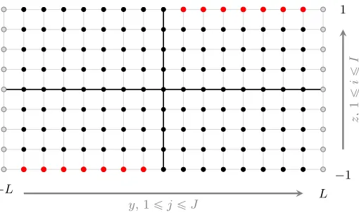
Figure 2. Discretization of DY “ p´1,1q ˆ p´Y, Yq and D˘Y “ t˘1u ˆ p´Y, Yq. At black points, the discretized equation is satisfied. At grey points, homogeneous Neumann boundary conditions are used, and at red points non-standard boundary conditions are employed.

with

´pLyuqi,jfi´ 1 2

ˆ

ui,j`1´2ui,j`ui,j´1

δy2

˙

´maxp0, bi,jq

ˆ

ui,j`1´ui,j

δy

˙

´minp0, bi,jq

ˆ

ui,j´ui,j´1

δy

˙

where bi,j “ ´pc0yj`kziq. The nonlocal Dirichlet boundary conditions (second condition) in (5) and in (13) at the red points in Figure 2are discretized by the same formulae withL replaced byL˘, wherepL˘uqi,j are defined by

´ pL`uqi,jfi´pLyuqi,j´minp0, yjq

ˆ

ui,j´ui´1,j

δz

˙

(21)

and

´ pL´uqi,jfi´pLyuqi,j´maxp0, yjq

ˆ_u

i`1,j´ui,j

δz

˙

. (22)

Note that, unlike [11,27], we are not able to guess the value of uand uλ or its derivative on the boundaries

y“ ˘Y. Instead, we proceed as in [32] in imposing an homogeneous Neumann condition. This is based on the intuition that, whenY is chosen sufficiently large, the probability of finding the underlying process outside the truncated domain is negligible. This idea is supported by Monte Carlo simulations as shown below.

The Neumann boundary conditions at the points shown in grey in Figure2 results in

pN2uqi,j“0, where pN2uqi,jfi

$ ’ ’ ’ &

’ ’ ’ %

ui,j`1´ui,j

δy ifj“1,

ui,j´ui,j´1

δy ifj“J.

(23)

We also do the following modification : gi,j“0 at the grey points. For the time dependent problem, this results in the following nonlinear system to be solved in each time step:

min`

Mδtun`

1

´gn_δt, un`1´f˘

“0, u0“f, (24)

and for the stationary problem

min`

HereMδt is a sparseNˆN-matrix that depends onδtbut not onn. Precisely, using the notation

lpi, jqfij` pi´1qJ, Gfitpi, jq, iP t1, . . . , Iu, jP t1, Juu, R´fitp1, jq, jP t2. . .J˜uu,

R`fitpI, jq, jP tJ˜`2. . . J´1uu, Bfit1, . . . , Iu ˆ t1, . . . , Ju ´ pGYR´YR`q.

‚ for everynP t1, . . . , NTuand for every pointpi, jq PG,pgδtnqi,j“0. Otherwise,pgnδtqi,j“ pun`δtgqi,j.

‚ for every grey point labeled bypi, jq PG,

– Mδtplpi,1q, lpi,1qq “ ∆1y,Mδtplpi,1q, lpi,2qq “ ´

1 ∆y

– Mδtplpi, Jq, lpi, Jqq “ ∆1y,Mδtplpi, Jq, lpi, J´1qq “ ´

1 ∆y

‚ for every black point labeled bypi, jq PB,

– Mδtplpi, jq, lpi´1, jqq “ ∆∆ztminp0, yjq

– Mδtplpi, jq, lpi, j´1qq “ ´∆t

´ 1 2∆y2 ´

min_p0,bi,jq ∆y

¯

– Mδtplpi, jq, lpi, jqq “1`∆t

´ 1 ∆y2 `

|bi,j| ∆y `

|yj| ∆z

¯

– Mδtplpi, jq, lpi, j`1qq “ ´∆t

´ 1 2∆y2 `

max_p0,bi,jq ∆y

¯

– Mδtplpi, jq, lpi`1, jqq “ ´∆∆ztmaxp0, yjq

‚ for every red point labeled bypi, jq PR´,

– Mδtplp1, jq, lp1, j´1qq, Mδtplp1, jq, lp1, j`1qq, Mδtplp1, jq, lp2, jqqhave the same expression than in the black points case butMδtplp1, jq, lp1, jqq “1`∆t

´ 1 ∆y2 `

|b1,j| ∆y `

minp0,yjq ∆z

¯

.

‚ for every red point labeled bypi, jq PR`,

– MδtplpI, jq, lpI´1, jqq, MδtplpI, jq, lpI, j´1qq, MδtplpI, jq, lpI, jqq, MδtplpI, jq, lpI, j`1qqhave the same expression than in the black points case but MδtplpI, jq, lpI, jqq “ 1`∆t

´ 1 ∆y2 `

|bI,j| ∆y `

maxp0,yjq ∆z

¯

.

The construction ofMλis very similar. For the computational results presented in the remainder of this paper, we use aC _{code that implements a Monte Carlo (MC) probabilistic simulation to approximate the solution of}

(1). We use aMATLAB_{implementation for the PDE approach (24). Implementations are available upon request.}

3.2.2. Case of the HJB problems (10)and (14)

We proceed as what was done above, except that we need to incorporate the control in the upwinding differences. The first conditions in (10) and (14) at the black points in Figure2 result in

v_i,j0 “fi,j and min

αPA ˜

v_i,jn`1´vn i,j

δt ´

`

Lαvn`1˘_i,j´gi,j

¸

“0, 0ďnďNT ´1, (26)

and min αPA ´ λvλ i,j´ `

Lvλ˘_i,j´gi,j

¯

“0, (27)

where

´pLαuqi,jfi´pLyαuqi,j´maxp0, yjq

ˆ

ui`1,j´ui,j

δz

˙

´minp0, yjq

ˆ

ui,j´ui´1,j

δz

˙

with

´pLα_yuqi,j fi´ 1 2

ˆ

ui,j`1´2ui,j`ui,j´1

δy2

˙

´maxp0, αi,j`bi,jq

ˆ

ui,j`1´ui,j

δy

˙

´minp0, αi,j`bi,jq

ˆ

ui,j´ui,j´1

δy

˙

Again, the nonlocal Dirichlet boundary conditions (second condition) in (10) and (14) at the red points in Figure2 are discretized by the same formulae withLα _{replaced byL}α

˘ defined by

´pLα_`uqi,jfi´pLyαuqi,j´minp0, yjq

ˆ

ui,j´ui´1,j

δz

˙

and

´pLα_´uqi,jfi´pLyαuqi,j´maxp0, yjq

ˆ

ui`1,j´ui,j

δz

˙

.

Also, we impose a Neumann boundary condition at the points shown in grey as in (23). Here, for the time dependent problem, this results in the following nonlinear system to be solved in each time step:

min α

`

M_δtαun`1´gn_δt˘

“0, u0“f, (28)

and for the stationary problem

min α

`

M_λαuλ´g˘

“0, (29)

where the matrices M_δtα and M_λα are almost the same matrices as Mδt and Mλ, except that b is replaced by

b`α.

4.

_{Numerical results}

4.1.

Free boundary value problems

We consider the case shown in (3) which is related to the problem (5) withλ“0.1,g“0 andf “1t|z|“1_u. This

quantity is the probability that the elasto-plastic system has entered, at least once, in the plastic phase before the instantT. Roughly speaking, as long as it remains small, it is somehow reasonable to approximate statistics of the elasto-plastic system by using those of a linear system. By solving (24), a numerical approximation for

up0,0, tnqof (5) is obtained. For comparison, a probabilistic numerical approximation of the left hand side in (3) is provided as an alternative method to the deterministic approach. The numerical results are shown in Figure3. Note that in contrast with the Monte Carlo approach, the PDE approach also computes upxi, yj, tq,@i, j, as presented in Figure4(withλ“0.1). Figure5displays the shape of the optimal stopping decision. We see that, except for the initial time, the optimal stopping decision is constant in time. Recall that, following the notations introduced in Section 3, 1 corresponds to stopping and 0 to continuing. We see that the optimal decision is to stop when the process reaches the plastic boundary and to continue otherwise. Note that the process never reaches the regions where signpyqz“ ´1 hence the value of the control in these regions does not matter.

4.2.

HJB problems

We consider both cases shown in (4) which are related to the problem (10) withλ“0.1,fpz, yq “0 and

‚ either gpz, yq “ |y|1t|z|“1u (accumulated plastic deformation),

‚ orgpz, yq “1t|z|“1u (time spent on the plastic boundary).

By solving (28), a numerical approximation forvp0,0, tnqof (10) is obtained. We do not have explicit solutions for the problems we are studying here and we cannot compute them using a straightforward probabilistic approach. However, for checking, we consider a numerical approximation of an optimal controlαoptp.qsatisfying

Jpαoptp.qq “sup

α E

˜ żT

0

gpz_sα, y_sαqds

¸

.

The approximation of αopt is obtained from the PDE solution. Then we have used it as an input in the probabilistic numerical scheme to approximateE´şT0 gpz

αopt

s , yαsoptqds

¯

0 1 2 3 4 5 6 7 0

0.2 0.4 0.6 0.8 1 1.2

TimeT

u

p

0

,

0

,T

q

PDE MC

Figure 3. Comparison of the PDE (solid) approach solving the free boundary value problem (5) and MC (dashed) approach based on the right hand side of (3). Approximation of the valuesup0,0, TqandP0,0pDtP r0, Ts,|zt| “1qare shown forT P r0,7s.

of Monte Carlo simulations based on an Euler discretization of the dynamics (8) controlled by αopt, see e.g. Bernardin [15] for more details. This method has given satisfactory results in the sense that the empirical expectation computed by the probabilistic method matches the corresponding value ofusolving (28) computed by the deterministic method. In order to check the convergence of the method, we compute the residual in the sup-norm for (28) withpuopt, αoptqobtained numerically with the above PDE method, that is

max i,j,n

`

pI`δtpM`Mαopt_qqun`1

opt ´unopt´δtg

˘

i,j.

For a grid of 400 time steps andI“J “150, we obtain a residual of the order of 10´12_.

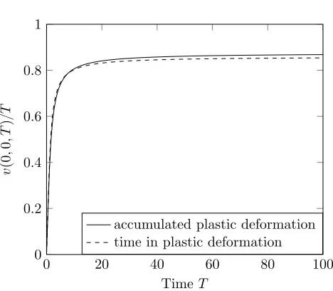
Figure 6, shows the graph of vp0,0, Tq{T for T P r0,100s, computed by the PDE method described in Section 3, for the two test cases accumulated plastic deformation (i.e. gpz, yq “ |y|1t|z|“1_u) and time spent on the plastic boundary(i.e. gpz, yq “1t|z|“1_u). One can see that for largeT, the time spent in plastic deformation

is smaller than the accumulated plastic deformation. This is because for large time, even when it starts from

p0,0q, the process has a high probability to reach large values of|y|on the boundary|z| “1 and when|y| ą1, the running cost of the test case time spent on the plastic boundary is smaller than the running cost of the other test case. Figure7shows the time evolution of the value function for theaccumulated plastic deformation

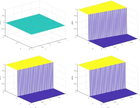
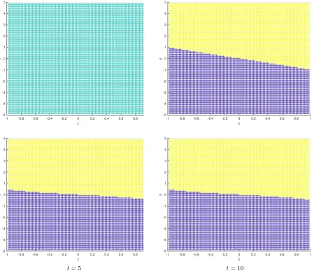
test case (with λ“0.1). The range of the value function keeps increasing with time because with longer time horizon, the process will accumulate more plastic deformation. However, for a given z, the value function is increasing with respect to |y|. This can be explained as follows: when the process starts closer to the plastic boundary, it is more likely to accumulate a lot of plastic deformation, which is reflected by the value function of this problem. The shape optimal control (at the final time t “100) is displayed in Figure 8 (3d plot) and Figure 9 (2d plot). One can see that, roughly speaking, the optimal decision is to push the process towards the closest portion of the plastic boundary. One can see that the control is ´1 in a region and`1 in another region. The line between them crosses the quadrant tpy, zq:y ą0, z ă0uand tpy, zq: y ă0, zą0u and, as

0 5 0.2 0.4

1

u

0.6

0.5

y

0 0.8

z

0 1

-0.5 -5 -1

t“0

0 5 0.2 0.4

1

u

0.6

0.5

y

0 0.8

z

0 1

-0.5 -5 -1

t“1

0 5 0.2 0.4

1

u

0.6

0.5

y

0 0.8

z

0 1

-0.5 -5 -1

t“5

0 5 0.2 0.4

1

u

0.6

0.5

y

0 0.8

z

0 1

-0.5 -5 -1

t“10

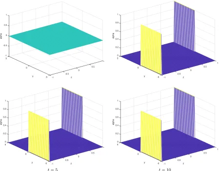
Figure 4. FB problem as shown in (5) : evolution of the value function in time upy, z, tq. The shots are taken at different times t “0,1,5,10. The terminal condition is f “1_t|z|“1_u,

the right hand sideg“0 andλ“0.1.

corresponding evolution of the optimal control. One can see that the value of the optimal control switches between´1 and`1. Moreover, the value`1 is applied, roughly speaking, in the upper half of the phase space, while the value ´1 is applied in the lower part. This is consistent with Figures8–9.

The value function and the optimal control for the problem of the time spent in the plastic deformation are very similar to those obtained for the case of accumulated plastic deformation so we omit them. Furthermore, we have also solved the ergodic problems (free boundary value problem and Hamilton-Jacobi-Bellman problem) and checked that the value functions of dynamic problems converge to the one of the corresponding ergodic problems.

5.

_Conclusion

-1 -0.5

0 0.5

1

z

-5 0

5

y

-1 -0.5 0 0.5 1

alpha

t“0

0 5 0.2 0.4

1

alpha

0.6

0.5

y

0 0.8

z

0 1

-0.5 -5 -1

t“1

0 5 0.2 0.4

1

alpha

0.6

0.5

y

0 0.8

z

0 1

-0.5 -5 -1

t“5

0 5 0.2 0.4

1

alpha

0.6

0.5

y

0 0.8

z

0 1

-0.5 -5 -1

t“10

Figure 5. FB problem as shown in (5): evolution of the optimal stopping decision ˆapz, y, tq

as shown in (6) and (7). The shots are taken at different times t “ 0,1,5,10. It consists in stopping (value 1) when the process reaches the plastic boundary and continuing otherwise (value 0). The terminal condition isf “1t|z|“1u, the right hand side is g“0 andλ“0.1.

accumulated plastic deformation (see Figure8). Second, we could consider more general control problems (in this work, as a first step we have considered only a control acting linearly on the drift, see (8)). In particular, computing solutions for the problems (2) remains a challenging task.

Acknowledgements

0 20 40 60 80 100 0

0.2 0.4 0.6 0.8 1

TimeT

v

p

0

,

0

,T

q{

T

accumulated plastic deformation time in plastic deformation

Figure 6. Approximation of the values ofvp0,0, Tq{T forT P r0,100s obtained by the PDE approach solving the HJB problem (10) for both problems accumulated plastic deformation

(solid line) andtime spent on the plastic boundary (dashed line).

Department of Mathematics of the City University of Hong Kong for the hospitality. JW acknowledges support from the SAR Hong Kong grant [CityU 11306115] “Dynamics of Noise-Driven Inelastic Particle Systems”.

References

[1] R. Bellman, Functional equations in the theory of dynamic programming. V. Positivity and quasi-linearity, Proc. Natl. Acad. Sci. USA, 41 (1955), pp. 743746.

[2] R. Bellman, Dynamic Programming, Princeton University Press, Princeton, NJ, 1957.

[3] A. Bensoussan, J-L. Lions, Contrˆole impulsionnel et in´equations quasi variationnelles. Dunod, Paris 1982.

[4] A. Bensoussan, L. Mertz, O. Pironneau, J. Turi, An Ultra Weak Finite Element Method as an Alternative to a Monte Carlo Method for an Elasto-Plastic Problem with Noise, SIAM J. Numer. Anal. , 47(5) (2009), 3374–3396.

[5] A. Bensoussan, L. Mertz, Degenerate Dirichlet problems related to the ergodic theory for an elasto-plastic oscillator excited by a filtered white noise, IMA J. Appl. Math. (2015) 80 (5): 1387-1408.

[6] A. Bensoussan, L. Mertz, An analytic approach to the ergodic theory of stochastic variational inequalities, C. R. Acad. Sci. Paris Ser. I, 350(7-8), (2012), 365–370.

[7] A. Bensoussan, C. Feau, L. Mertz, S.C.P. Yam, An analytical approach for the growth rate of the variance of the deformation related to an elasto-plastic oscillator excited by a white noise, Appl. Math. Res. Express (2015) (1): 99-128.

[8] A. Bensoussan, L. Mertz, S.C.P. Yam, Long cycle behavior of the plastic deformation of an elasto-perfectly-plastic oscillator with noise, C. R. Acad. Sci. Paris Ser. I, 350(17-18), (2012), 853–859.

[9] A. Bensoussan, L. Mertz, S.C.P. Yam, Nonlocal problems related to an elasto-plastic oscillator excited by a filtered noise, SIAM J. Math. Anal. 48-4 (2016), pp. 2783-2805.

[10] Blumenthal, R. M.; Getoor, R. K., Markov processes and potential theory, Pure and Applied Mathematics, Vol. 29 Academic Press, New York-London (1968).

[11] O. Bokanowski, S. Maroso, H. Zidani, Some convergence results on Howard’s algorithm, SIAM. J. Num. Analysis, vol. 47(4), pp. 3001-3026.

[12] A. Bensoussan, J. Turi, Degenerate Dirichlet Problems Related to the Invariant Measure of Elasto-Plastic Oscillators, Applied Mathematics and Optimization,58(1)(2008), 1–27.

[13] A. Bensoussan, J. Turi, On a Class of Partial Differential Equations with Nonlocal Dirichlet Boundary Conditions, Appl. Num. Par. Diff. Eq.15, pp. 9-23.

[14] B.K. Bathia, E.H. Vanmarcke, Associate linear system approach to nonlinear random vibration, J. Engrg. Mech., ASCE, 117, (1991), 2407-2428.

-1 -0.5

0 0.5

1

z

-5 0

5

y

-1 -0.5 0 0.5 1

u

t“0

0 5 0.5 1

1 1.5

u

2

0.5

y

0 2.5

z

0 3

-0.5 -5 -1

t“1

1 5 1.5 2 2.5

1 3

u

3.5

0.5 4

y

0 4.5

z

0 5

-0.5 -5 -1

t“5

1 5 2 3

1

u

4

0.5

y

0 5

z

0 6

-0.5 -5 -1

t“10

Figure 7. HJB problem as shown in (10): evolution of the value function in time vpz, y, tq

for the accumulated plastic deformation. The shots are taken at different times t“0,1,5,10. The terminal condition isf “0, the right hand side isg“ |y|1_t|z|“1_u andλ“0.1.

[16] L. Borsoi, P. Labbe Approche probabiliste de la ruine d’un oscillateur ´elasto-plastique sous s´eisme. 2`eme colloque national de l’AFPS. 18-20 Avril 1989.

[17] G.Q. Cai, Y.K. Lin, On randomly excited hysteretic structures, J. of Applied Mechanics, ASME 57, (1990), 442-448. [18] T.K. Caughey, Nonlinear theory of random vibrations, Adv. in Appl. Mech.11, C.S. Yih (ed.), Academic Press, (1971), 209-253. [19] O. Ditlevsen, Elasto-Plastic oscillator with Gaussian excitation, J. of Engrg. Mech., ASCE, 112, (1986), 386-406.

[20] O. Ditlevsen, L. Bognar, Plastic displacement distributions of the Gaussian white noise excited elasto-plastic oscillator, Prob. Eng. Mech. 8, (1993), 209-231.

[21] O.Ditlevsen, N. Tarp-Johansen, White noise excited non-ideal elasto-plastic oscillators, Acta Mechanica 125, (1997), 31-48. [22] G. Duvaut, J.L. Lions, Inequalities in Mechanics and Physics, Springer-Verlag, New-York, 1976.

[23] C. Feau, Probabilistic response of an elastic perfectly plastic oscillator under Gaussian white noise, Probabilistic Engineering Mechanics,23(1)(2008),36–44.

[24] C. Feau, L. Mertz An empirical study on plastic deformations of an elasto-plastic problem with noise, Probabilistic Engineering Mechanics, (30) (2012), 60–69.

[25] R. Grossmayer, Stochastic analysis of elasto-plastic systems, J. Engrg. Mech., ASCE, 39, (1981), 97-115. [26] R.A. Howard, Dynamic Programming and Markov Processes, The MIT Press, Cambridge, MA, 1960.

-1 -0.5

0 0.5

1

z

-5 0

5

y

-1 -0.5 0 0.5 1

alpha

t“0

-1 5 -0.5

1 0

alpha

0.5 0.5

y

0

z

0 1

-0.5 -5 -1

t“1

-1 5 -0.5

1 0

alpha

0.5 0.5

y

0

z

0 1

-0.5 -5 -1

t“5

-1 5 -0.5

1 0

alpha

0.5 0.5

y

0

z

0 1

-0.5 -5 -1

t“10

Figure 8. HJB problem as shown in (10): evolution of the optimal control in time ˆapz, y, tq

for the accumulated plastic deformation. The shots are taken at different times t“0,1,5,10. The terminal condition isf “0, the right hand side isg“ |y|1_t|z|“1_u andλ“0.1.

[28] D. Karnopp, T.D. Scharton, Plastic deformation in random vibration, The Journal of the Acoustical Society of America,39

(1966), 1154-61.

[29] B. Lazarov, O. Ditlevsen, Slepian simulation of distributions of plastic displacements of earthquake excited shear frames with large number of stories, Prob. Eng. Mech. 20, (2005), 251-262.

[30] C. Feau, M. Lauri`ere, L. Mertz, Asymptotic formulae for the risk of failure related to an elasto-plastic problem with noise, Asymptotic Analysis, 106, (2018), 47-60.

[31] R.H. Lyon, On the vibration statistics of a randomly excited hard-spring oscillator II, J. Acoust. Soc. Amer. 33 (1961), 1395-1403.

[32] L. Mertz, G. Stadler, J. Wylie, A backward Kolmogorov equation approach to compute means, moments and correlations of non-smooth stochastic dynamical systems, arxiv.org/abs/1704.02170.

[33] A. Preumont, Random Vibration and Spectral Analysis, Kluwer, Boston, 1994.

[34] J.B. Roberts, The response of an oscillator with bilinear hysteresis to stationary random excitation, J. of Applied Mechanics 45, (1978), 923-928.

[35] J.B. Roberts, Reliability of randomly excited hysteretic systems, Mathematical Models for Structural Reliability Analysis, F. Casciati and J.B. Roberts (eds.), CRC Press, 1996, 139-194.

[36] J.B. Roberts, P.D. Spanos, Random Vibration and Statistical Linearization, Wiley and Sons, Chichester, U.K., 1990. [37] B.F. Spencer, Reliability of Randomly Excited Hysteretic Structures, Springer-Verlag, Berlin, 1986.

-1 -0.8 -0.6 -0.4 -0.2 0 0.2 0.4 0.6 0.8 1 z

-5 -4 -3 -2 -1 0 1 2 3 4 5

y

t“0

-1 -0.8 -0.6 -0.4 -0.2 0 0.2 0.4 0.6 0.8 1 z

-5 -4 -3 -2 -1 0 1 2 3 4 5

y

t“1

-1 -0.8 -0.6 -0.4 -0.2 0 0.2 0.4 0.6 0.8 1 z

-5 -4 -3 -2 -1 0 1 2 3 4 5

y

t“5

-1 -0.8 -0.6 -0.4 -0.2 0 0.2 0.4 0.6 0.8 1 z

-5 -4 -3 -2 -1 0 1 2 3 4 5

y

t“10

Figure 9. HJB problem as shown in (10): evolution of the optimal control in time ˆapz, y, tq

for the accumulated plastic deformation (view from above). The shots are taken at different timest“0,1,5,10. The terminal condition isf “0, the right hand side isg“ |y|1t|z|“1u and

λ“0.1.

[39] N. Touzi, Optimal Stochastic Control, Stochastic Target Problems, and Backward SDE Springer-Verlag, New York, 2013. [40] E.H. Vanmarcke, On the distribution of the first-passage time for stationary random processes, Journal of Applied Mechanics,

(1975), 215–220.

-1 -0.8 -0.6 -0.4 -0.2 0 0.2 0.4 0.6 0.8 1

-0.2 -0.15 -0.1 -0.05 0 0.05 0.1 0.15

y

z

alpha = 1 alpha = -1 no control

(a)Trajectories

-1 -0.5 0 0.5 1

0 0.1 0.2 0.3 0.4 0.5 0.6 0.7 0.8 0.9 1 1.1

alpha

t

(b)Optimal control

Figure 10. HJB problem as shown in (10): Left: one realization of a trajectory with the optimal control (full line) and without control (dashed line) for the same realization of the noise; right: corresponding evolution of the optimal control in time ˆαt “ ˆapzt, yt, tq for the accumulated plastic deformation. The terminal condition is f “ 0, the right hand side is