Volume 61, 2019, Pages 183–200
ARCH19. 6th International Workshop on Applied Verification of Continuous and Hybrid Systems
Worst-Case Analysis of Digital Control Loops
with Uncertain Input/Output Timing
Maximilian Gaukler and Peter Ulbrich
Friedrich-Alexander-Universit¨at Erlangen-N¨urnberg, Germany [email protected],[email protected]
Abstract
Benchmark Proposal: The implementation of digital control systems in complex multi-core or distributed real-time systems results in non-deterministic input/output timing. Such timing deviations typically lead to degraded performance or even instability, which in turn may jeopardize safety goals. We present the problem of proving worst-case guar-antees for given input/output timing bounds as a benchmark for the verification of hybrid dynamical systems.
1
Introduction
Digital control implements feedback control on a computing system. Its defining characteristic is that reading sensor inputs and actuating the resulting control signal are performed at discrete points in time. Therefore, a common design assumption is the simultaneous and strictly periodic execution of these two steps. As automatic control is particularly sensitive to timing variations, a real-time computing system is used in safety-critical applications to assure temporal properties and thus a predictable quality of control.
However, while deterministic timing simplifies the design of the control system, its im-plementation is becoming increasingly difficult from a real-time systems’ perspective. Recent developments, such as distributed real-time systems, multicore platforms, and smart sensors, come at the cost of increasing complexity and degrading predictability. Consequently, the syn-chronous design approach to digital control becomes excessively expensive. A common solution to this issue is to resort to input/output (IO) windows, that is timing bounds instead of de-terministic time instants. In turn, we have to verify that the resulting timing variations do no jeopardize the aspired safety and stability of the feedback control even in the worst case.
In this paper, we present worst-case verification of digital control loops with uncertain IO timing as a benchmark problem for the verification of hybrid automata. Therefore, we detail the system model in section2 and translate it to a hybrid system in section3. Finally, formal goals and multiple examples are introduced in section4.
2
System Model
For a formal description of the problem, we adapt the timing model of [10], which was used for stochastic average-case analysis, to the setting of worst-case stability verification. The main differences are a generalisation to nonlinear systems and the removal of reference tracking.
Plant The physical system to be controlled is described as a time-invariant plant, for which
the following nonlinear equations and their linear special case, denoted bylin=, are given.
˙
xp(t) =fp(xp(t), u(t), d(t)) lin
=Apxp(t) +Bpu(t) +Gpd(t), t >0,
y(t) =gp(xp(t), d(t)) lin
=Cpxp(t) +Hpd(t). (1)
The plant has input u(t) = u1(t) u2(t) . . . um(t) T
∈ Rm, state xp(t) ∈ Rnp and output
y(t) =
y1(t) . . . yp(t) T
∈Rp. Ap, Bpet cetera are matrices of appropriate dimension. The
initial statexp(0)∈Xp,0⊂Rnpis unknown but bounded. Disturbance and measurement noise are modeled by a bounded, nondeterministic inputd(t)∈D ⊂Rndist. If they are not present, this will later be denoted byndist= 0, which means that the dependency ond(t) and the terms
Gpd(t) andHpd(t) are omitted.
Controller The plant is controlled by the discrete-time controller
xd[k+ 1] =fd(xd[k], y[k]) lin
=Adxd[k] +Bdy[k], xd∈Rnd,
u[k] =gd(xd[k]) lin
=Cdxd[k], xd[0] = 0, k∈N0 (2)
with nominal periodT. This formulation includes standard linear controllers, such as discretized PID or observer-based state feedback. The given form has no feedthrough, which means that the control signalu[k] only requires the previous measurementy[k−1]. This restriction is reasonable for control systems in which timing is relevant, as it permits a computation time of slightly below one control period, while with feedthrough any computation time would inevitably delay the output. For simplicity and due to the goal of stability analysis, we only consider a constant set point ofy= 0.
IO timing model Nominally, the whole measurement vectory[k] is sampled att=kT. From this, the control signalu[k+ 1] is computed and then emitted att= (k+ 1)T. The real timing differs from this: The j-th control output component is delayed by ∆tu,j[k] (where negative
values represent a too early output), which can formally be stated as
uj(t) = (
uj[k], kT+ ∆tu,j[k]< t <(k+ 1)T+ ∆tu,j[k+ 1] ∧ k≥1
Tb[k−1] kT Tb[k]
t
∆t...[k]
dataflow
virtual dependency Sampley[k−1] Sample y[k] Sampley[k+ 1]
Compute
u[k]
Compute
u[k+ 1]
Actuateu[k] Actuateu[k+ 1] Actuateu[k−1]
Figure 1: Timing model for IO and computation with dataflow dependencies, the timing barrier
Tb[k] and its corresponding virtual dependencies.
Respectively, the sampleyj[k] of thej-th sensor is acquired with a time offset ∆ty,j[k].
yj[k] = (
yj(kT+ ∆ty,j[k]), k≥1
0, else. (4)
The “0” case in eqs. (3) and (4) is only relevant for start-up and will be discussed later.
The timing of input, computation and output and its dataflow dependencies (double arrows) are shown in fig.1. As a “black-box” model, the timing of each input and output component is unknown but bounded:
∆tu,j ≤∆tu,j[k]≤∆tu,j, ∆ty,j ≤∆ty,j[k]≤∆ty,j ∀j, k≥1 (5)
Additional constraints, e. g., that a group of inputs is always sampled at the same time, may be considered to make the model less pessimistic, but are not discussed here for the sake of clarity.
To avoid the need for extra buffers in the realization and corresponding buffer states in the resulting model, neighboring cycleskandk+ 1 are separated by a timing barrierTb[k], which
no event may cross:
kT+ ∆ty,j[k]
kT+ ∆tu,j[k]
<Tb[k]<
(k+ 1)T+ ∆ty,j[k+ 1]
(k+ 1)T+ ∆tu,j[k+ 1]
∀j, k≥1 (6)
This barrier coincides with the controller computation and can equivalently be described by a task with zero execution time and four virtual dependencies as shown in fig.1. To simplify the subsequent model, we only consider Tb = (k+ 12)T in the following, which means that each
location
ODE invariant
location2
ODE2
invariant2 label
guard
jump
Figure 2: Legend for hybrid automata used in this publication
Startup behavior Because time doesn’t start at t =−T /2, but at t = 0, the first half of the cycle k = 0 is missing, and yj[0] would not be sampled if ∆ty,j[0] < 0. To avoid this
discontinuity, samplingy[0] and actuatingu[0] are skipped, which is reflected in the “0” case of eqs. (3) and (4). Because the startup behavior only affects a finite time interval at the start, changing it is roughly equivalent to a change of the initial set. For the linear case, it is therefore not relevant for infinite-time, e. g. asymptotic stability.
3
Hybrid Automata
The system model presented in the previous section can be equivalently formulated as the interconnection of multiple hybrid automata, which is a precise and machine-readable formal description suitable for automatic verification. A simplified summary of the semantics of hybrid automata will be given in the following. We refer to [8] for an extended introduction and to [11] for a strict formalization.
Semantics A hybrid automaton as shown in fig.2combines a discrete-event automaton with a classical continuous-time, continuous-valued dynamical system. In each location (discrete-valued state) of the discrete-event automaton, the state variables of the continuous system evolve according to an ordinary differential equation (ODE) and are restricted to a set given by an invariant condition. A transition to another locationmay be taken while the associated guard condition is true (may-semantics) and must be taken before the invariant condition of the current location is violated. At the transition, the continuous state changes instantaneously as given by the jump transition, e. g.,x0 = 2xstates thatxjumps to twice its previous value. For synchronization of multiple automata, labels are used: If multiple transitions have the same nonempty label, either all are executed at once or none of them.
Nondeterminism Because the timing is bounded but otherwise unknown, the system is non-deterministic: Multiple trajectories are possible for a given disturbance and initial state. The nondeterminism of may-semantics mentioned before is used to represent the nondeterminism of IO timing. This would be significantly more difficult ifmust-semantics (urgent semantics)
were used instead, which defines that transitions must be taken as soon as possible.
3.1
Components
0 T 2T
T
2
0
−T
2
t τ
0
xd,unext
(a) Behavior.
always
˙
τ = 1, x˙d = 0
−T /2 ≤ τ ≤ T /2
startOfCycle
τ = T /2
τ0 = −T /2, x0d = fd(xd, yd)
(b) Hybrid Automaton.
controller and clock
τ, startOfCycle
unext=gd(xd)
yd
(c) Block diagram.
Figure 3: Specification of controller and clock
Controller and Clock As in depicted in fig.3a, we define the periodic sawtooth clock signal
τ = ((t+T /2) modT)−T /2, (7) which is the signed distancet−kT to the nearest nominal sampling pointkT. This signal is generated by the automaton from fig. 3b, which also includes the controller: τ continuously increases ( ˙τ = 1) untilτ=T /2 is reached, which is the timing boundaryt= (k+1/2)Tbetweeen two control cycles. Then,τis reset fromT /2 to−T /2 and the new controller state is computed from the recent measurement. This event is given a synchronization labelstartOfCycle, which will later be used to force the reset of all sample-and-hold automata.
A block diagram representation is shown in fig.3c. The input is the sampled measurement
yd. The outputs are the clock τ, the labelstartOfCycle, which corresponds to the falling edge
ofτ, and the “next” (most recently computed) control signalunext=gd(xd).
Generic sample-and-hold (SH) The transitions between discrete-time controller and con-tinuous-time plant can be modeled by SH elements as shown in figs. 4a and 4b. The output
b is updated to the value of the input a once per period, within ∆t ≤ τ ≤ ∆t, and held constant inbetween (˙b= 0). In accordance with the timing model, the parameters ∆t and ∆t
are restricted to−T /2<∆t≤∆t < T /2.
This description is implemented by the automaton in fig. 4c, which uses may-semantics to model that sampling may happen while ∆t ≤τ ≤∆t andmust happen before τ >∆t. The
startOfCyclesynchronization label, which occurs at the transition fromτ =T /2 toτ=−T /2, is used to reset the automaton at the beginning of each cycle.
Plant The plant is described the equations given in section2:
˙
SH(∆t,∆t)
a
τ,startOfCycle
b
(a) Block diagram.
0 (T+ ∆t) T (T+ ∆t) 2T
t
a(t)
b(t), earliest
b(t)
b(t), latest
(b) Behavior.
wait
˙
b = 0
τ ≤ ∆t
done
˙
b = 0 ∆t ≤ τ ≤ ∆t
b0 = a
startOfCycle
(c) Hybrid automaton.
Figure 4: Specification of sample-and-hold (SH) element
3.2
Interconnection
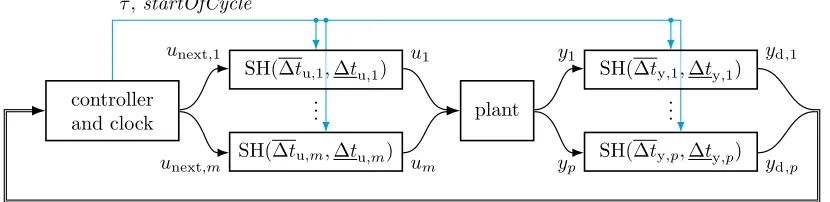
The closed loop is modeled by connecting controller and plant with one sample-and-hold block per input and output component as shown in fig.5. All timing-dependent components share the common clockτ and the correspondingstartOfCycle synchronization label.
In this block diagram, controller and plant are interconnected with unext = gd(xd) and
y = gp(xp, d). Such interconnection variables, which are not needed as state variables, may
introduce additional computational effort in analysis. Therefore, a different but equivalent implementation was used for the experiments described later: The statesxd andxp were used
as interconnection and the computation ofgp(...) andgd(...) was moved into the SH components.
3.3
Initialization and Startup
The controller is initialized atxd= 0, τ = 0, and all SH automata start in location “done” with
stateb= 0. The plant state is bounded byxp(0)∈Xp,0. The SH automata are initialized at
location “done” to match to the specified behavior of skipping the cyclek= 0.
Alternative startup behavior A different startup behavior could be modeled by starting at τ =−T /2 and “wait”, which would be equal to starting at t= T /2 with the first regular cyclek= 1. It is not generally possible to initializeτ = 0 and still use “wait” as initial location, because the invariantτ ≤∆twould be violated at start if ∆t <0.
4
Benchmark Setup
τ,startOfCycle
controller and clock
.. .
SH(∆tu,1,∆tu,1)
SH(∆tu,m,∆tu,m)
plant ...
SH(∆ty,1,∆ty,1)
SH(∆ty,p,∆ty,p)
unext,1
unext,m
u1
um
y1
yp
yd,1
yd,p
Figure 5: Block diagram of closed control loop
Given A digital control loop with uncertain but bounded input/output timing and distur-bance as modeled in section2, equivalent to the hybrid system described in section3.
Goal 1: Stability proof Prove practical stability of the control loop, which we define as that for bounded initial state, the infinite-time reachable set
S :=n
xTp(t) xTd(t) u
T(t) yT(t)T
t≥0, dynamics of section3, with uncertainties
xp(0)∈Xp,0, ∆t...[k]∈
∆t...; ∆t...
, d(ξ)∈D∀ξo (9) is bounded. For a quadcopter, this means that there is a proven, possibly large, bound on the worst-case position error. For any linear controller and plant, this implies marginal or exponential stability, if the internal timingτ is not considered a state.
Practical stability can be shown with set-valued reachability analysis by finding a bounded
upper approximation ¯S⊇S of the reachable set.
Goal 1b: Exponential decay Prove global uniform exponential stability of the controlled plant: For zero disturbance (ndist= 0 orD={0}), find constantsC, λ >0 such that
kxp(t)k2≤Ce−λtkxp(0)k2 ∀t≥0, ∀xp(0). (10)
While practical stability only ensures that the state is bounded, exponential stability is desirable because it guarantees a certain rate of decay for the initial error.
Goal 2: Tight bounds If the system is stable, compute useful bounds on the states
xp, xd, u, y: For a quadcopter, the analysis must prove that worst-case position error is less
than a few centimeters, not kilometers. In general, this guaranteed and thereforeouter bound ¯
S⊇S obtained from analysis should be not much larger than aninner approximationS ⊆S
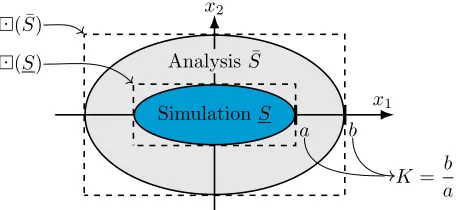
from a large number of random simulations. As a metric for usefulness, we introduce the bloating factorK, the worst ratio of the component-wise bounds of analysis and simulation:
K:= max
j
max
x∈S¯ eTjx
max
x∈S eTjx
, whereej denotes thej-th unity vector. (11)
An equivalent definition is illustrated in fig.6:
x2
x1
SimulationS
( ¯S)
(S) Analysis ¯S
a b
K= b
a
Figure 6: Illustration of the metricK, which compares the interval bounds of simulation and pessimistic analysis.
where (·) denotes the enclosing symmetric multidimensional interval (symmetric box). An ideal verification tool can achieveK= 1 in short computation time. K1 corresponds to a large undesirable gray area between analysis and simulation, in which the existence of trajectories can neither be confirmed nor denied.
Goal 2b: Extreme examples Efficiently finding extreme simulation traces to show minimal
Kis a problem on its own. Ideally, a verification tool should provide concrete examples of the worst case to show that its result is not unnecessarily pessimistic.
4.1
Approximate Continuous-Time Variant
For comparison, we provide a purely continuous variant of the problem: Assuming perfect timing and a negligibly small periodT, the discrete-time difference quotient of the controller statexdis approximated by a continuous-time differential equation. Witht=kT, this yields
˙
xd(t)≈
xd[k+ 1]−xd[k]
T =
fd(xd[k], y[k])−xd[k]
T
lin
=Ad−I
T xd(t) + Bd
T y(t). (13)
The new closed loop does not require states for measurement and actuation and is given by
˙
xp(t)
˙
xd(t)
lin
=
Ap BpCd
T−1BdCp T−1(Ad−I)
˙
xp(t)
˙
xd(t)
+
Gp
T−1BdHp
d(t). (14)
We remark that the stability of this system is neither sufficient nor necessary for the stability of the original, discrete-time system. However, modeling the difference between (14) and the orig-inal system as bounded disturbance could yield a continuous-time abstraction (continuization) of the original controller, similar to [5].
4.2
Examples and Experiments
5
Summary and Outlook
Uncertain input/output timing adversely affects the performance of digital control loops but is virtually unavoidable in complex real-time systems. To still prove safety we are required to prove worst-case behavior, such as the maximum position error of a quadcopter, in the presence of timing uncertainty. To address this challenge, we present a series of benchmark problems for the verification of hybrid automata, which are a formalism that captures both the discrete-time and continuous-discrete-time aspects of real-discrete-time control systems. However, first experiments with set-based reachability tools suggest that verification is only possible for simple examples.
Set-based reachability analysis typically performs overapproximations at discrete transitions to keep computational effort acceptable. This suggests that it is best suited for systems with few discrete transitions and stable continuous dynamics; the opposite of this is the case for digital control loops. Our experiment substantiates this hypothesis, raising the question of whether we are faced with a fundamental problem or if a tailored verification approach or modified algorithms can solve the issues.
While numerous techniques for the verification of discrete-time controllers exist, to the best of our knowledge, none of them supports timing uncertainties as presented in our model, which addresses real-time systems with multiple sensors and actuators. Therefore, future work will entail an extension of existing techniques. One candidate is continuization [5], a method for approximating discrete-time controllers as continuous-time controllers with disturbance, which are more suitable for reachability analysis. Further candidates are LMI-based methods for linear control systems as discussed in [12].
References
[1] Matthias Althoff. An introduction to CORA 2015. In Goran Frehse and Matthias Althoff, editors, ARCH14-15. 1st and 2nd International Workshop on Applied veRification for Continuous and Hybrid Systems, volume 34 ofEPiC Series in Computing, pages 120–151. EasyChair, 2015. [2] Stanley Bak, Sergiy Bogomolov, and Taylor T. Johnson. HYST. In Proceedings of the 18th
International Conference on Hybrid Systems Computation and Control - HSCC'15. ACM Press, 2015.
[3] Stanley Bak and Marco Caccamo. Computing reachability for nonlinear systems with HyCreate. 16th International Conference on Hybrid Systems: Computation and Control Poster Session, 2013. [4] Stanley Bak and Parasara Sridhar Duggirala. HyLAA: A tool for computing simulation-equivalent reachability for linear systems. In Proceedings of the 20th International Conference on Hybrid Systems: Computation and Control, HSCC ’17, pages 173–178, New York, NY, USA, 2017. ACM. [5] Stanley Bak and Taylor T. Johnson. Periodically-scheduled controller analysis using hybrid systems
reachability and continuization. In2015 IEEE Real-Time Systems Symposium. IEEE, 2015. [6] Xin Chen, Erika ´Abrah´am, and Sriram Sankaranarayanan. Flow*: An analyzer for non-linear
hybrid systems. In International Conference on Computer Aided Verification, pages 258–263. Springer, 2013.
[7] A. E. C. Da Cunha. Benchmark: Quadrotor attitude control. In Goran Frehse and Matthias Althoff, editors, ARCH14-15. 1st and 2nd International Workshop on Applied veRification for Continuous and Hybrid Systems, volume 34 ofEPiC Series in Computing, pages 57–72. EasyChair, 2015.
[9] Goran Frehse, Colas Le Guernic, Alexandre Donz´e, Scott Cotton, Rajarshi Ray, Olivier Lebeltel, Rodolfo Ripado, Antoine Girard, Thao Dang, and Oded Maler. SpaceEx: Scalable verification of hybrid systems. InInternational Conference on Computer Aided Verification, pages 379–395. Springer Berlin Heidelberg, 2011.
[10] Maximilian Gaukler, Andreas Michalka, Peter Ulbrich, and Tobias Klaus. A new perspective on quality evaluation for control systems with stochastic timing. InProceedings of the 21st Interna-tional Conference on Hybrid Systems: Computation and Control (part of CPS Week) - HSCC'18. ACM Press, 2018.
[11] T.A. Henzinger. The theory of hybrid automata. InProceedings 11th Annual IEEE Symposium on Logic in Computer Science, pages 278–292. IEEE Comput. Soc. Press, July 1996.
[12] Laurentiu Hetel, Christophe Fiter, Hassan Omran, Alexandre Seuret, Emilia Fridman, Jean-Pierre Richard, and Silviu Iulian Niculescu. Recent developments on the stability of systems with aperi-odic sampling: An overview. Automatica, 76:309–335, February 2017.
A
Source Code and Data Files
The source code and output data used in this publication is available online athttps://doi. org/10.5281/zenodo.2600139. Updated versions will be provided athttps://github.com/ qronos-project/arch19-benchmark-iotiming.
B
Example Data
In the following, example systems are presented. For reference, the systems are denoted by a letter, followed by a number indicating the variant. To limit implementation complexity and the number of variants, we restrict the examples to linear systems and only consider variants without disturbance in the subsequent experiments.
Note: SpaceEx model files for this section can be found incode/template/output/, e. g.,
code/template/output/solved with spaceex/stable/A1 1.spaceex.xmlfor example A1.
B.1
One-dimensional Example (A1)
For an example of minimal dimensionsn=nd =m=p= 1, a linear, weakly unstable plant
Ap = 0.05, Bp = 0.5, Cp = 1, without disturbance (ndist = 0) is controlled by the
discrete-time controller Ad=−0.01, Bd=−0.4, Cd= 1. The timing is uncertain (∆ty =−0.1,∆ty =
0.002,∆tu =−0.001,∆tu = 0.002) and the initial state is bounded within the intervalXp,0 =
[−1; 1]. It should be noted that even for this one-dimensional plant and controller, the resulting hybrid system has 4 continuous state variables (xp, u, yd, xd).
The parameters of this system were heuristically chosen such that SpaceEx can verify stabil-ity via an invariant set within seconds with optimized settings and within minutes with almost arbitrary settings. Variants with increased and decreased difficulty are also provided:
A2 Negligible jitter: ∆tu,y=−∆tu,y= 0.0001
A3 Increased jitter: ∆tu=−0.4,∆tu= 0.1,∆tu=−0.1,∆tu= 0.4 A4 Extreme jitter: Variant A3 with ∆tu= 0.4
A5 Increased dimension: Variant A3 is duplicated, which means that all dynamics matrices are diagonally repeated such asAp,A5= diag(Ap,A3, Ap,A3). This increases the dimension
A6 Disturbance (not included in experiments): To add disturbance and measurement noise, the system may be changed tondist= 2, Gp=1 0, Hp=0 1, D= [−1; 1]2.
B.2
Trivial Three-dimensional Example (B1)
For an example of higher order, a stable three-dimensional plant is combined with a controller that has negligible influence on the plant dynamics:
Ap=
−1 0.002 0.003 0.004 −5 0.006 0.007 0.008 −9
, Bp=
0.001 0.0011 0.0012 0.0013 0.0014 0.0015
, Cp=16 17 18 (15)
Ad=
0.019 0.02 0.021 0.022
, Bd=
0.023 0.024
, Cd=
0.025 0.026 0.027 0.028
(16)
T = 2, ∆tu=−∆tu=
0.2 0.4
, ∆ty =−∆ty= 0.6, Xp,0= [−1; 1]3, ndist= 0 (17)
Variant B2: Disturbance (not included in experiments) To add input disturbance, the system may be changed tondist= 1, Gp=
1 0 0T
, Hp=
0 0T
, D= [−1; 1].
B.3
Quadcopter Examples (C, D)
The linearized dynamics of the angular rate control of a quadcopter, mostly based on [7], are the basis for two models. Angular rate control is an important subsystem of quadcopter stabilization, which ensures that the rate of rotationrφ, rθ, rψaround thex,yandzaxis follows
the setpoint given by a higher-level control system. For simplicity, the latter is not considered here and instead the setpoint is assumed to be zero. For a detailed system description and physical model, we refer to [7] and the references provided there.
Single-axis angular rate control (C) If only the rotationφaround thex-axis is considered, the mechanical dynamics of the angular raterφ are
Jφr˙φ(t) =Tφ(t) (18)
with rotational inertiaJφ. The input is the time-varying torqueTφ(t) controlled by the motors
and the output is the angular raterφ(t) measured by a gyroscope.
The original, continuous-time controller
Tφ(t) =−Kp,φrφ(t)−KI,φ Z t
0
rφ(ξ)dξ (19)
given in [7] is discretized in a simplified way as
Tφ[k] =−KP,φrφ[k−1]−KI,φ k−1 X
0
rφ[k]. (20)
To match the timing model,Tφ[k] has no feedthrough, i. e., it does not depend on the current
Three-axis angular rate control (D) If all three axes of rotation are considered, the linearized dynamics are three independent integrators
Jφr˙φ(t) =Tφ(t), (21)
Jθr˙θ(t) =Tθ(t), (22)
Jψr˙ψ(t) =Tψ(t). (23)
The torquesTφ,θ,ψ and the vertical thrustFz are controlled by the forces u1,2,3,4 of four
pro-pellers, which are defined as inputs to the system because rotor dynamics are neglected:
Tφ(t)
Tθ(t)
Tψ(t)
Fz(t) =
0 −l 0 l
−l 0 l 0
γ −γ γ −γ
1 1 1 1
| {z }
M
u1(t)
u2(t)
u3(t)
u4(t)
| {z } u(t)
. (24)
This equation depends on the distancel between center and rotor and the ratioγof torque to rotor thrust. Because altitude control is not considered here, we setFz= 0 and obtain
u(t) =M−1
Tφ(t)
Tθ(t)
Tψ(t)
0 , (25)
where Tφ,θ,ψ(t) is each computed by a PI controller in the structure of eq. (20), but with
axis-dependent controller parameters.
It should be noted that for perfect timing, the system can be split into three decoupled subsystems, whereas if the components of u(t) are not updated synchronously, the control torque of one axis slightly affects other axes.
While the presented model is highly simplified, our experiments in verifying it were not suc-cessful. As soon as it has been successfully verified, more realistic variants should be considered, e. g., by adding disturbance, nonlinearities, rotor dynamics and position control.
Parameters The original publication [7] states the following parameters: Jφ = 9.036·10−6,
Jθ= 9.127·10−6,Jψ = 1.937·10−5,KP,φ= 2.557·10−4, KP,θ= 2.581·10−4,KP,ψ = 5.478·10−4,
KI,φ= 3.614·10−3,KI,θ = 3.651·10−3, KI,ψ= 7.747·10−3.
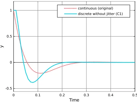
We assume l = 0.1 and γ = 0.01, which are not given in [7] and therefore chosen within the order of magnitude observed in other quadcopter models. The controller period is chosen asT = 0.01, which is a compromise between a response similar to the original continuous-time controller and low processor utilization. The initial response of the original and the discretized controller are compared in fig.7.
The dynamics matrices for example C are
Ap= 0, Bp= 1.107·105, Cp= 1, (26)
Ad=
1 0 0 0
, Bd=
1·10−2
1
, Cd=
−3.614·10−3 −2.556·10−4
Figure 7: Initial responserφ(t) of original and discretized controller for example C for an initial
staterφ(0) = 1 and perfect timing.
(Simulink simulation: code/template/example C simulation of nominal case.slx)
and for example D are
Ap=
0 0 0
0 0 0
0 0 0
, Bp=
0 −1.107·104 0 1.107·104 −1.096·104 0 1.096·104 0
5.163·102 −5.163·102 5.163·102 −5.163·102
, (28)
Cp=
1 0 0
0 1 0
0 0 1
, Ad=
1 0 0 0 0 0
0 0 0 0 0 0
0 0 1 0 0 0
0 0 0 0 0 0
0 0 0 0 1 0
0 0 0 0 0 0
, Bd=
1·10−2 0 0
1 0 0
0 1·10−2 0
0 1 0
0 0 1·10−2
0 0 1
, (29) Cd=
0 0 1.825·10−2 1.291·10−3 −1.937·10−1 −1.370·10−2
1.807·10−2 1.279·10−3 0 0 1.937·10−1 1.370·10−2
0 0 −1.825·10−2 −1.291·10−3 −1.937·10−1 −1.370·10−2 −1.807·10−2 −1.279·10−3 −2.533·10−18 −1.791·10−19 1.937·10−1 1.370·10−2
. (30)
We assume no disturbance (ndist= 0) and an initial state withinXp,0= [−1; 1]np. Two timing
variants are provided:
C1, D1 Perfect timing: ∆tu,y= ∆tu,y= 0
C2, D2 The timing may vary by ±0.01T: ∆tu,y=−∆tu,y= 0.01T1 1 . . . T
.
B.4
Timer Example (E)
For debugging and visualization, the following example can be used. The plant is a timer with output y(t) = xp,1(t) = t, regardless of the input. Therefore, it is obviously unstable. The
controller isu[k+ 1] =y[k]. Becauseuhas no effect ony, this results inu[k+ 1] =kT+ ∆ty[k].
the measurement was sampled. The parameters are given in the following:
Ap=
0 1 0 0
, Bp=
0 0
, Cp=
1 0
, Xp,0=
0 1
, ndist = 0 (31)
Ad= 0, Bd= 1, Cd= 1 (32)
T = 1, ∆tu=−0.4, ∆tu= 0.1, ∆ty=−0.2, ∆ty= 0.3 (33)
C
Experiments
First, a selection of tools is evaluated in appendixC.1. All examples presented in this publication are then evaluated with the selected candidates, SpaceEx and Pysim, in appendixC.2.
Computation times were measured on a 3.6 GHz Intel Core i7-4790 CPU, running on Ubuntu 18.04 with a memory limit of 14 GB. For model files, tool settings and output see appendixA.
C.1
Selection of Tools
We restricted our experiments to SpaceEx [9] and a small number of open-source set-valued reachability tools for which a conversion from SpaceEx exists. The SpaceEx tool was used as a starting point because it directly supports the modeling scheme used in section 3. The one-dimensional example A1 from appendix B.1 was created in the format of SpaceEx. For use with other tools, it was converted using Hyst [2]. As most other tools don’t support the interconnection of multiple automata, this conversion also includes computing the synchronous product to yield a single equivalent automaton.
Note: Code and data for this section can be found incode/dummy/.
SpaceEx With manually optimized settings, which can be found in code/dummy/a1.cfg, SpaceEx 0.9.8f successfully finds the fixpoint for the reachable set shown in fig. 8 after few seconds. As mentioned earlier, the parameters of example A1 were specifically chosen such that verification with SpaceEx is possible, so this result is by design. Further experiments with SpaceEx can be found in the next section.
Flowstar By design, the Flowstar [6] tool only supports bounded-time reachability computa-tion. As a workaround, convergence of the desired infinite-time reachable set was approximated by comparing the reachable set for finite time horizons from 5 to 100. The time step setting was varied from 10−1 to 10−4, where the latter already requires one hour of computation time
for a time horizon of 10.
We were unable to obtain useful results with Flowstar 2.0.01, even for negligible timing uncertainties as in example A2: For a time horizon of 10, the resulting set was already five times bigger than the infinite-time result of SpaceEx, and for larger time horizons Flowstar did not finish within a run-time limit of two hours. However, it cannot be completely ruled out that this is due to an unfortunate choice of parameters.
Figure 8: Reachable set (y overτ) computed by SpaceEx for example A1
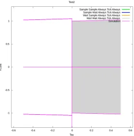
HyCreate According to its website2, the HyCreate [3] tool has been discontinued and is not recommended for more than three continuous states for longer time horizons. Nevertheless, a short experiment was carried out. After correcting syntax errors in Hyst’s output, HyCreate 2.81 returned a reachable set that only covers τ > 0, which means that the periodic reset transition τ0 = −T /2 is never taken. A similar result was shown by HyCreate’s integrated simulation engine. After weakening the guard condition τ =T /2 to τ ≥0.9T /2, the region −T /2< τ <0 is reached by simulations, but still not contained in the computed reachable set (see fig.9), which suggests an error in HyCreate or Hyst. The corresponding files can be found incode/dummy/hycreate2/.
Hylaa As of January 2019, the stable version of Hylaa [4] (55a72f8, “master” branch) does not yet support resets, which means the state must not change at a transition. Therefore Hylaa is not suitable for our model. While the current development version (“hybrid” branch) seems to support transitions, it could not be used because it is not yet supported by Hyst. However, it is a promising candidate for future experiments.
CORA Due to a misunderstanding, we assumed that CORA [1] does not support the may-semantics used by our model and therefore excluded it from our experiments. We will, however, include it in future experiments provided online.
Pysim The Pysim simulator supplied with Hyst uses must-semantics, as can be seen from its source code. However, as Pysim only simulates, this only means that it will constantly use the earliest possible timing, which is technically correct but not representative of the set of possible trajectories.
Figure 9: Erroneous reachable set (yoverτ) returned by HyCreate: The simulation (lines) goes outside the computed reachable set (shaded area), which does not reachτ <0. The model file can be found atcode/dummy/hycreate2/test2-converted-fixed.hyc2.
To simulate a pseudo-random selection of trajectories without requiring extensive modifi-cations to Pysim, a modified version of the model was created, in which the guard condition ∆t≤τ≤∆tin may-semantics was changed toτ ≥∆t+r(∆t−∆t) in must-semantics, where
r∈[0; 1] is a pseudo-random number updated at the beginning of each cycle. To fit the existing framework of Pysim and Hyst without extensive modifications, this was approximated by
r0= 0.5 + 0.5 cos(1234r), (34)
which is a prototypical, weak pseudo-random number generator, whose seed value is the initial state of r. Each SH subcomponent has a separate random state, and the initial values are varied to obtain different trajectories.
Additionally, because the equality guard condition τ =T /2 is not correctly simulated due to numerical issues, it was changed toτ≥T /2, which is equivalent in must-semantics.
C.2
Evaluation of Examples
np nd m p timing SpaceEx tSE KSE LTI-stable
A1 1 1 1 1 varying (small) X 1 s 1.010 —
A2 1 1 1 1 varying (negligible) X 1 s 1.001 —
A3 1 1 1 1 varying (medium) X 2 s 1.059 —
A4 1 1 1 1 varying (large) ×error (GLPK) — — —
A5 2 2 2 2 varying (like A3) ×crash (GLPK) — — —
B1 3 2 2 1 varying X 16 s 1.097 —
C1 1 2 1 1 constant ×timeout — — stable
C2 1 2 1 1 varying ×crash — — —
D1 3 6 4 3 constant ×diverging — — stable
D2 3 6 4 3 varying ×crash — — —
E 2 1 1 1 varying — — — unstable
Table 1: Experimental results.
np, nd, m, p: dimensions of plant, controller, input and output. timing: fixed or uncertain timing?
SpaceEx,tSE: result of SpaceEx and runtime (including computation of interval bounds). X: practically stable, neglecting floating point inaccuracy. ×: failed to verify practical stability. timeout: runtime exceeded two hours. diverging: reached K > 1000 without showing stability. crash: aborted due to unhandled error such as memory access or assertion violation. error: exited with error message. (GLPK: error is related to solving linear programs with the GLPK library)
KSE: Upper bound of K factor per eq. (11), comparing SpaceEx’ overapproximation and random Pysim simulations. Only applicable if SpaceEx verifies stability.
LTI-stability: stability proof by analysis of the time-discretized nominal case (∆t= 0), which is a linear time-invariant (LTI) system (—: not applicable for varying timing, except to show instability).
Note: Code and data for this section can be found incode/template/.
For each example, SpaceEx’ maximum number of iterations was adjusted such that either it found a fixpoint, states corresponding to K > 1000 were reached or a run-time limit of two hours was exhausted. If a fixpoint was found, this means that the system is practically stable, assuming that floating point computation inaccuracy in SpaceEx is negligible. The remaining settings were chosen as in the initial experiments, except for example B, which had to be changed to directions=box (set overapproximation as multidimensional interval) for successful verification. An exhaustive search for the best settings could not be performed in the scope of this work, which means that the presented results may be suboptimal.
The results in table1highlight that SpaceEx could verify stability only for the most simple examples (A1 – A3 and B) and fails otherwise.
The results point to three possible reasons for the encountered difficulties.
Firstly, increasing timing variation makes verification more difficult, as can be seen in ex-amples A1 – A4: Example A2 with almost constant timing is verified with almost no bloating, whereas increased timing in A3 leads to more bloating and runtime, and A4 with large timing cannot be verified.
To illustrate the effect of increased timing uncertainty on verification, the reachable set over global time t was computed by adding t as a state with ˙t = 1 and t(0) = 0. Figure10
highlights that in simulations (left), example A1 (top) shows about the same rate of decay for
y(t) as example A3 (bottom), whereas the reachable set (right) decays significantly slower. This matches the increasedK-factor observed in table1.
Figure 10: Comparison of random simulations y(t) (left) and the reachable set for y over t
computed by SpaceEx (right) for examples A1 (top) and A3 (bottom). Colors in the simu-lation refer to modes of the hybrid automaton. Input data for this figure can be found in
code/template/output/solved with spaceex/A{1,3} ....
Third, the dynamics of the nominal case (perfect timing), such as oscillating versus expo-nentially decaying, may play an important role: Example C1 has perfect timing and less states than B1, however, only B1 can be verified. While verification with SpaceEx fails for exam-ples C1 and D1, which have constant timing ∆t... = 0, they can easily be proven stable by
![Figure 1: Timing model for IO and computation with dataflow dependencies, the timing barrierTb[k] and its corresponding virtual dependencies.](https://thumb-us.123doks.com/thumbv2/123dok_us/8876437.1817141/3.612.136.474.103.287/figure-timing-computation-dataow-dependencies-barriertb-corresponding-dependencies.webp)