ISSN: 2008-6822 (electronic)
http://www.ijnaa.semnan.ac.ir
Some statistical inferences on the upper record of
Lomax distribution
G. Yari∗, Z. Karimi Ezmareh
Department of Mathematics, Faculty of Mathematics, Iran University of Science and Technology, Tehran, Iran
(Communicated by Madjid Eshaghi Gordji)
Abstract
In this paper, some inferential properties of the upper record of the Lomax distribution are inves-tigated. The upper record of the Lomax distribution parameters are estimated by using methods, Moment (MME), Maximum Likelihood (MLE), Kullback-Leibler Divergence of the Survival function (DLS) and Baysian. In addition, These methods are compared using Monte-Carlo simulation. Fi-nally, this new model is fitted on the real data and some of the comparative criteria are calculated to confirm the superiority of the proposed model to other models.
Keywords: Lomax distribution, Upper record, Entropy, Parameter estimation, Simulation.
2010 MSC: Primary 37Mxx, Secondary 65Cxx.
1. Introduction
One of the most widely used income distributions, especially in statistics, is the two-parameter Lomax distribution. This distribution, which is a special case of income distribution known as Singh-Maddala, was first introduced by Lomax in 1954 to investigate the performance of any business failure data. Lomax distribution is used in business, economics, real science, queuing theory, internet traffic modeling, and etc [2]. This distribution is more flexible than the classic Pareto distribution in fitting to income data. Since this distribution has only two parameters, and its cumulative distribution function (cdf) and its quantile function are simple, it can be easily interpreted relative to the Singh-Maddala distribution. Consequently, fitting to income data is very suitable. Ahsanullah [4] reviewed some of the distributional properties of the record values and moments up to second order of Lomax distribution. Balakrishnan and Ahsanullah [10] studied the relations for single and product moments
∗Corresponding author
Email addresses: [email protected](G. Yari∗),[email protected](Z. Karimi Ezmareh)
of record values from Lomax distribution. Interested readers can refer to Resources [7], [9], [27], [31], [29], [17], [24], [15], and [14] for more details.
Nowadays, the concept of records is used in many daily life issues such as weather, sports, geo-physics, seismology and so on. In fact, when we deal with sequential observations, that are more or less than their previous, values records are used. Records are very important when observations are difficult to obtain or when observations are being destroyed when subjected to an experimental test. The term record value was first introduced by Chandler [13]. The interested readers can refer to [6], [5], [8], [25], [30], [33], [20], [32], [22], [34], [21], and [18].
The term entropy in the word, refers to a change from order to disorder. The birth of the infor-mation theory can be attributed to Shannon’s ”mathematical theory of inforinfor-mation” article, 1948. Shannon stated in his article that the amount of uncertainty in a random experiment is measured by the entropy of possible outcomes. Nyquist [26] and Hartley [19] also conducted studies in this field. After the introduction of Shannon entropy, other criteria for measuring uncertainty were expressed by generalizing it. Among them, one can mention the Renyi entropy, Tsallis entropy, relative entropy and mutual information. Relative entropy (Kullback-Leibler Divergence (DLS)) was first introduced by Kullback-Leibler in 1951 [28], which measures the distance between two distributions.
In this paper, we use the various methods to estimate the parameters of upper record of Lomax distribution. For this purpose, we will use the relatively new DLS method. Finally, the results show that using the DLS method is more efficient in estimating the scale parameter.
Now, we carry out some necessary definition in the subsequent discusion [16], [1], [11], [28], [28], and [8].
Definition 1.1. If X is a random variable having an absolutely continuous cdf F(x), pdf f(x) and support Sx, then the Shannon entropy of X is defined
H(X) = −
∫
Sx
fX(x) logfX(x)dx. (1.1)
Definition 1.2. If X is a random variable having an absolutely continuous cdf F(x), pdf f(x) and support Sx, then Renyi entropy of order ρ of the random variable X is defined by
Hρ(X) = −
1 ρ−1log
∫
Sx
fρ(x)dx , ∀ρ >0(ρ̸= 1). (1.2)
Definition 1.3. If X is a random variable having an absolutely continuous cdf F(x), pdf f(x) and support Sx, then Tsallis entropy of orderρ of the random variable X is defined by
Sρ(X) =
1 ρ−1
[
1−
∫
Sx
fρ(x)dx
]
, ρ̸= 1, ρ >0. (1.3)
Definition 1.4. Let X1, X2, ... be a sequence of positive, independent and identically distributed (iid) random variable from a non-increasing survival function F¯(x,Θ) =PΘ(X > x)with support Sx
and vector of parameters Θ. Define the empirical survival function of a random sample of size n by
¯
Gn(x) = n−1
∑
i=0
I[X(i),X(i+1))(x), (1.4)
Definition 1.5. Let F¯(x,Θ) be the true survival function with unknown parameters Θ and G¯n(x)
be the empirical survival function of a random sample of size n from F¯(x,Θ). Define the Kullback-Leibler divergence of survival functions G¯n(x) and F by
DLS( ¯Gn∥F¯) =
∫ ∞
0
(¯
Gn(x) ln
¯ Gn(x)
¯
F(x) −[ ¯Gn(x)− ¯
F(x)])dx. (1.5)
Definition 1.6. LetX1, X2, ...be a sequence of iid random variables having an absolutely continuous cdf F(x) and pdf f(x). An observation Xj is called an upper record value if its value exceeds that of
all previous observations. Thus, Xj is an upper record if Xj > Xi for every i < j . If we use the
notation XU(n) for the rth upper record statistic then, the pdf of the XU(n) is
fXU(n)(x) =
[−ln(1−F(x))]n−1
Γ(n) f(x),−∞< x <∞, (1.6)
where Γ is the gamma function.
The rest of this paper is organized as follows. In the next section, some preliminary results and some studies on the entropy of the upper record values are presented, as well as the calculation of these results for the upper record of Lomax distribution (URLD). In section 3, we will estimate parameters of the URLD by using different methods. In section 4, we will compare the methods using the Monte Carlo simulation. Finally, in Section 5, by using a real data set, the uURLD will be compared to the upper record of several other income distributions.
2. The upper record value of Lomax distribution and its entropy
In this section, first, we introduce some preliminary results for the upper record values. In addition, some studies on the Shannon, Renyi and Tsallis entropies of the upper record values are expressed.
Corollary 2.1. (See [3]). If use of the U =−2 log [1−F(x)] transform in relation 1.6, we have
XU(n)
d
=FX−1
[
1−exp(−1 2χ
2 (2n))
]
. (2.1)
Corollary 2.2. (See [3]). The 100(1−ϵ)% confidence interval for XU(n) is
P
[
FX−1(1−exp(−1 2χ
2 (2n,ϵ2))
)
< XU(n)< FX−1
(
1−exp(−1 2χ
2
(2n,1−2ϵ))
)]
= 1−ϵ. (2.2)
Corollary 2.3. (See [3]). The pth quantile for 0< p <1 of X U(r) is
FX−1
U(n)(p) =F
−1[1−exp(−1
2F
−1
χ2 (2n)
(p))]. (2.3)
Theorem 2.4. (See [11]). Let {Xn, n ≥ 1} be a sequence of iid continuous random variables from
the distribution F(x) with density function f(x) and entropy H(X)<∞. Then for all n≥1
H(XUn) =
n−1
∑
i=1
(logi− n−1
i ) + (n−1)γ−ϕf(n−1), (2.4)
where
ϕf(n) =
∫ +∞
0
zn
n!e
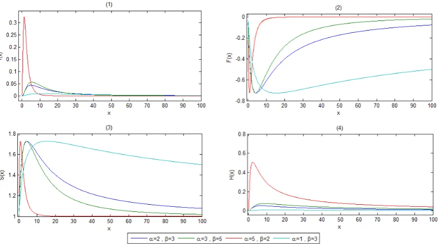
Figure 1: (1) Graph of pdf of 4thURLD for different values (α, β), (2) Graph of cdf of 4thURLD for different values
(α, β), (3) Graph of survival function of 4thURLD for different values (α, β), (4) Graph of hazard rate function of 4th
URLD for different values (α, β).
Theorem 2.5. (See [11]). Under the assumptions of theorem 2.4 we have
(i) H(XUn)≤H(XUn∗)−n−Bn−E[
logfY(y)
1−FY(y)
]−logM, (2.6)
(ii) H(XUn)≥H(XUn∗)−n−logM, (2.7)
where M =f(m)<∞, m is the mode of the distribution, Y =M X and
XUn∗ ∼Γ(n,1) , Bn=
(n−1)(n−1) (n−1)! e
−(n−1). (2.8)
Lemma 2.6. (See [1]). Let {Xn, n ≥1} be a sequence of iid continuous random variables from the
distribution F(x) with density function f(x) and the quantile functionF−1(.). Then the Renyi entropy of XU(n) can be expressed as
Hρ(XUn) =Hρ(XUn∗)−
ρ(n−1) + 1
ρ−1 logρ− 1
ρ−1logEgn [
fρ−1(F−1(1−e−vn))], (2.9)
where
XUn∗ ∼Γ(n,1) , vn∼gn= Γ(ρ(n−1) + 1,1). (2.10)
Lemma 2.7. (See [12]). Let X1, X2, ..., Xn be a random sample with size n from continuous cdf
F(x) and pdf f(x). Let XU(n) denotes the nth upper record. Then, the Tsallis entropy of XU(n) can be expressed as
Sρ(XUn) =
1 ρ−1
[
1−Γ(ρ(n−1) + 1)
Γρ(n) E(f
Now, we will study the upper record of Lomax distribution. A continuous random variable X is said to be a be a two-parameter Lomax distribution with shape parameter α and scale parameter β and denoted byX ∼Lomax(α, β), if its cdf is
F(x) = 1−(1 + x β)
−α ; x, α, β >0. (2.12)
In the following, based on the second section, we present the following results for the URLD:
1) Distribution of nth upper record is
XU(n)
d
=β[(exp(−χ
2 (2n)
2 ))
−1
α −1]. (2.13)
2) Probability density function XU(n) is
fXU(n)(x) =
αn
βΓ(n)[log(1 + x β)]
n−1(1 + x
β)
−(α+1). (2.14)
3) Survival function XU(n) is
¯
FXU(n)(x) = (
1 + x β
)−α n−1
∑
j=0
(
αlog(1 + x(i)
β
))j
j! . (2.15)
4) Hazard rate function XU(n) is
H(x) =
αn
βΓ(n)[log(1 +
x β)]
n−1(1 + x β)−
(α+1)
(
1 + x β
)−α∑n−1
j=0 1
j!
(
αlog(1 + x(i)
β
))j. (2.16)
5) Moment generating function XU(n) is
MXU(n)(t) =
∞ ∑ m=0 m ∑ k=0 tm m!α
nβm (−1) k(m
k
)
(α−m+k)n. (2.17)
6) The 100(1−ϵ)% confidence interval forXU(n) is
(
β[(exp(− χ2
(2n,ϵ2)
2 ))
−1
α −1], β[(exp(−
χ2 (2n,1−ϵ2)
2 ))
−1
α −1]). (2.18)
7) The pth quantile for 0< p <1 of X U(n) is
qU(n)(p) = β
[
(exp(−1
2Fχ2(2n)(p)))
−1 α −1
]
. (2.19)
8) Entropy of the upper record XU(n) is
H(XUn) =
n−1
∑
i=1
(logi− n−1
i ) + (n−1)γ −log( α β) +
n(α+ 1)
9) Bounds for entropy of the upper record values XU(n) is
H(XUn∗)−n−log(
α
β)≤H(Un)<∞. (2.21)
10) Renyi entropy of the upper record XU(n) is
Hρ(XUn) = Hρ(XUn∗)−
ρ(n−1) + 1
ρ−1 logρ−log α β +
ρ(n−1) ρ−1 log
(
ρ+ 1
α(ρ−1)
)
. (2.22)
11) Tsallis entropy of the upper record XU(n) is
Sρ(XUn) =
1 ρ−1
[
1− Γ(ρ(n−1) + 1)
Γρ(n) (
α β)
ρ−1[α+ 1
α (ρ−1) + 1]
−ρ(n−1)−1
]
. (2.23)
3. Estimation of parameters of the URLD
In this section, we use four methods to estimate the shape parameter α and the scale parameter β of the URLD. Suppose that X1, X2, ..., Xn is a random sample from rth upper record of Lomax
distribution.
Moment method (MME):
In this method, after equating the moments of population and the sample, we have the following equations:
(I) x¯=β
[
( α
α−1)
r−1
]
,
(II) x¯2 =β2
[
( α
α−2)
r−2( α
α−1)
r+ 1
]
,
(III) s2 =β2
[
( α
α−2)
2r−( α
α−1)
r
]
.
Here, we consider three cases:
• Ifα is known and β is unknown, according to equation (I), the estimator β is
˜
βαknown =
¯ x
[
( α α−1)
r−1]. (3.1)
• Ifβ is known andα is unknown, according to equation (I), the estimator α is
˜
αβknown = [1−(1 +
¯ x β)
−1
r]−1. (3.2)
• If α and β are both unknown then, equating the sample coefficient of variation (CV) and the population CV (we observe that the population CV is independent of the β) we have
CV =
√
V ar(X) E(X) =
s ¯ x =
√
(αα−2)r−( α α−1)2r
(αα−1)r−1 , (3.3)
where ¯x= n1 ∑ni=1xi and s2 = n−11
∑n
i=1(xi −x)¯
2. Now, using equation 3.3 and with the help
Maximum Likelihood method (MLE):
In this method, the logarithm of the likelihood function for the URLD is
logL=nrlogα−nlogβ+ (r−1)
n
∑
i=1
log[log(1 + xi
β)]−(α+ 1)
n
∑
i=1
log(1 + xi
β). (3.4)
Now, we have to maximize the 3.4 to the parameters. In this method, we consider three cases:
• If β is known and α is unknown: differentiate with respect to α then, equating to zero and solving with respect α. Then, the estimate of the MLE of parameter α is obtained as follows
ˆ
α= ∑n nr
i=1log(1 +
xi
β)
. (3.5)
• If α is known and β is unknown: again differentiate with respect to β then, equating to zero and solving with respect β. Then, the estimate of the MLE of parameter β is obtained as follows
∂logL
∂β =−n−(r−1)
n
∑
i=1
xi
β+xi
log(1 + xi
β)
+ (α+ 1)
n
∑
i=1
xi
β+xi
= 0. (3.6)
The solution of the above equation, which is a function based only onβ, yields the estimate of the MLE of parameter β by using appropriate numerical methods.
• Ifαandβ are both unknown then, in this case, by setting 3.5 in 3.4 and then taking a derivative of it with respect to β, we have
∂logL ∂β =nr
∑n i=1
xi
β+xi ∑n
i=1log(1 +
xi
β)
−n−(r−1)
n
∑
i=1
xi
β+xi
log(1 + xi
β) + n ∑ i=1 xi
β+xi
= 0. (3.7)
By solving this equation, which is a function based only onβ, yields the estimate of the MLE of parameter β by using appropriate numerical methods. Then by putting it in 3.5, the MLE estimate of the parameterα can also be calculated.
Bayesian Method:
To estimate the URLD in the Bayesian method, we assume the previous information ofα and β are independent of each other, so π(α, β) = π(α)π(β). In this method, we use the three prior distribu-tions uniform, normal and triangular (increasing and decreasing) using the Monte Carlo simulation (In the relevant section, the results are presented).
Kullback-Leibler Divergence of Survival function method (DLS):
In order to estimate the rth URLD by using DLS method, by replacing with ¯FXU(r) (the survival
function of rth upper record) in equation 1.5, it is as follows
DLS =
n−1
∑
i=0
(1− i
n) log(1− i
n)∆xi+1−
[
¯ xn−β
(
( α
α−1)
r−1)]
+ αβ n n ∑ i=1 (
(1 + x(i)
β ) log(1 + x(i)
β )− x(i)
β
)
−
n−1
∑
i=0
(1− i n)
∫ x(i+1)
x(i)
log
(∑r−1
j=0
(
αlog(1 +βx))j j!
)
where ∆xi+1 =xi+1−xi and x0 = 0.
We must now minimize DLS to parametersα and β. As a result, we have the following equations:
∂DLS
∂α = −
βrαr−1 (α−1)r+ 1 +
β n n ∑ i=1 (
(1 + x(i)
β ) log(1 + x(i)
β )− x(i)
β
)
−
n−1
∑
i=0
(1− i n)
∫ x(i+1)
x(i)
log
(∑r−1
j=0
αj−1(log(1 + xβ))j (j −1)!
)
dx= 0, (3.9)
∂DLS
∂β = −1 + α n n ∑ i=1 (
(1 + x(i)
β ) log(1 + x(i)
β )− x(i)
β ) − α nβ n ∑ i=1
x(i)log(1 +
x(i)
β )
+ ( α
α−1)
r− n−1
∑
i=0
(1− i n)
∫ x(i+1)
x(i)
∑r−1
j=0
xα β2 (
αlog(1+xβ)) j−1
(j−1)!
∑r−1
j=0
(
αlog(1+xβ)
)j
j!
dx= 0. (3.10)
Solving the above equations, using appropriate numerical methods, leads to the DLS estimation of the parameters α and β.
4. Simulation studies
According to the results, estimating the parameters using these methods does not have a closed form. As a result, appropriate numerical methods can be applied to evaluate the performance of these methods. For this purpose, MATLAB software is used.
First, we generate the random sample x1, x2, ..., xn from the 4th URLD with αtrue = 5 and
βtrue = 7. Then, we estimate the parameters with the help of the above methods. Now, we repeat
this process j = 10000 times. Finally, the sample mean values ¯α and ¯β and the sample variance s2
α and s2β are calculated for the comparison of the mentioned methods. Where αk and βk are the
estimated 4th URLD shape and scale parameter from kth sample. Certainly, the method in which
¯
α αtrue and
¯
β
βtrue are closer to one, provides more unbiased estimators.
In the Baysian method, note that for all three prior distributions, in the denominator of posterior distributions we have a dual integral, which is not a simple calculation. To overcome this problem, the ”importance sampling ” method is used. To investigate the effect of sample size on estimates, the above process is repeated for samples of size n = 10,20,30, ...,100 and the results are shown in Figures 2 and 3.
Comparison of α estimators:
• According to Figure 2 (a), the use of MME, MLE and Baysian methods, especially with the normal and increasing triangular prior, yields estimators very close to the real value. In the MLE method, for the small sample size, the estimators differ slightly from the actual value. But, with increasing sample size, they are very close to the real value.
• According to of Figure 2 (c), which shows αα¯
true, this ratio has a very close to one in methods
Figure 2: Comparison ofαestimators.
• According to of Figure 2 (b) and (d), the MLE (with increasing sample size) and Baysian methods have a lower Mean Square Error (MSE) than other methods. These two criteria also confirm the appropriateness of these two methods.
Comparison of β estimators:
• According to Figure 3 (e), the use of the DLS and Baysian methods, especially with the normal prior, yields estimators very close to real value. Other methods provide some estimators that are slightly different from the real value. However, in β estimation, the DLS method has a relatively good performance. Also, the MLE method has a better performance with increasing sample size.
• According to Figure 3 (g), which shows ββ¯
true, this ratio, in all methods, except for MME, has
a value close to one.
• According to Figure 3 (f) and (h), MLE (with increasing sample size), DLS and Baysian methods have the lowest MSE.
5. Application with real data set
In this section, by using a real data set, the URLD with the Upper Record of Pareto Distri-bution(URPD), Upper Record of Weibull Distribution(URWD) and Upper Record of Sing-Maddala Distribution(URSMD) are compared with the probability density function of:
fU RLD(x) =
αn
βΓ(n)[log(1 + x β)]
n−1(1 + x
β)
−(α+1); x >0, α, β > 0,
fU RP D(x) =
αnβα
Γ(n) 1 xα+1
[
log(1 + x β)
]n−1
; x≥β , α, β >0,
fU RW D(x) =
α βΓ(n)(
x β)
nα−1 ; x >0, α, β >0,
fU RSM D(x) =
αλn
β
[
log(1 + (x β)
α)]n−1(x
β)
α−1(1 + (x
β)
α)−(λ+1) ; x >0, α, β, λ >0.
These data include 14 records of the income (1959 dollars) of families for whites for the period 1949-1966, and derived from Source [23]. These data are:
4.188,4.332,4.513,4.720,4.935,5.083,5.398,5.633,5.732,5.828,6.086,6.294,6.534,6.750.
Table (1.1), contains the values of Akaike Information Criterion (AIC), Baysian information crite-rion(BIC) and contains goodness of fit test statistics Kolmogorov-Smirnov (K-S) with its correspond-ing p-value. The required numerical evaluations are implemented uscorrespond-ing the R software. As you can see in Table (1.1), the smallest values of information criterion values and goodness of fit test statistics and the largest p-value are related to the URLD. Therefore, it can be concluded that the URLD, in fitting this data, performs better than other distributions.
6. Conclusion
Table 1: Goodness of fit test statistics for mean income level of families for whites (1949-1966).
Distribution AIC BIC K-S P-Value
URLD 9.361821 10.63994 0.3156798 0.08901
URPD 9.920529 11.19864 0.5048093 0.0007909
URWD 10.82335 12.10146 0.8876496 1.023e-13
URSMD 14.5175 15.79562 134.3688 <2.2e−16.
parameters in four methods, MME, MLE, DLS, and Bayesian, and compared these estimators with Monte Carlo simulation, and showed that, in theαestimate, the use of the Baysian method with the appropriate prior and the method of MLE (in large sample size), leads to suitable estimators and in β estimation, the use of DLS, Baysian with the appropriate prior and MLE (in large sample size) methods is recommended. Finally, to prove the superiority of the URLD performance, compared to some other income distributions, we fitted this model to the real data and showed that the URLD, in fitting these data, was more appropriate than the URPD, URWD, and URSMD.
References
[1] M. Abbasnejad and N. R. Arghami. R´enyi entropy properties of records. Journal of Statistical Planning and Inference, 141(7):2312–2320, 2011.
[2] B. Afhami and M. Madadi. Shannon entropy in generalized order statistics from pareto-type distributions.
International Journal of Nonlinear Analysis and Applications, 4(1):79–91, 2013.
[3] J. Ahmadi and N. Balakrishnan. Confidence intervals for quantiles in terms of record range.Statistics & probability letters, 68(4):395–405, 2004.
[4] M. Ahsanullah. Record values of the lomax distribution. Statistica Neerlandica, 45(1):21–29, 1991.
[5] M. Ahsanullah. Record values of independent and identically distributed continuous random variables. Pak. J. Statist, 8(2):9–34, 1992.
[6] M. Ahsanullah. Record statistics. Nova Science Publishers, 1995.
[7] M. Arendarczyk, T. J. Kozubowski, and A. K. Panorska. A bivariate distribution with lomax and geometric margins. Journal of the Korean Statistical Society, 47(4):405–422, 2018.
[8] B. C. Arnold, N. Balakrishnan, and H. N. Nagaraja. Records., volume 768. John Wiley & Sons, 2011.
[9] M. N. Asl, R. A. Belaghi, and H. Bevrani. Classical and bayesian inferential approaches using lomax model under progressively type-i hybrid censoring. Journal of Computational and Applied Mathematics, 343:397–412, 2018. [10] N. Balakrishnan and M. Ahsanullah. Relations for single and product moments of record values from lomax
distribution. Sankhy¯a: The Indian Journal of Statistics, Series B, pages 140–146, 1994.
[11] S. Baratpour, J. Ahmadi, and N. R. Arghami. Entropy properties of record statistics.Statistical Papers, 48(2):197– 213, 2007.
[12] S. Baratpour and A. Khammar. Results on tsallis entropy of order statistics and record values. ˙Istatistik T¨urk
˙Istatistik Derne˘gi Dergisi, 8(2):60–73, 2016.
[13] K. Chandler. The distribution and frequency of record values. Journal of the Royal Statistical Society: Series B (Methodological), 14(2):220–228, 1952.
[14] G. M. Cordeiro, A. Z. Afify, E. M. Ortega, A. K. Suzuki, and M. E. Mead. The odd lomax generator of distributions: Properties, estimation and applications. Journal of Computational and Applied Mathematics, 347:222–237, 2019.
[15] G. M. Cordeiro, E. M. Ortega, B. V. Popovi´c, and R. R. Pescim. The lomax generator of distributions: Properties, minification process and regression model. Applied Mathematics and Computation, 247:465–486, 2014.
[16] T. M. Cover and J. A. Thomas. Elements of information theory. John Wiley & Sons, 2012.
[17] E. Cramer and A. B. Schmiedt. Progressively type-ii censored competing risks data from lomax distributions.
Computational Statistics & Data Analysis, 55(3):1285–1303, 2011.
[19] J. Hartley. Communication, cultural and media studies: The key concepts. Routledge, 2012.
[20] Z. Jaheen. Empirical bayes analysis of record statistics based on linex and quadratic loss functions. Computers & Mathematics with Applications, 47(6-7):947–954, 2004.
[21] J. Jose and E. A. Sathar. Residual extropy of k-record values. Statistics & Probability Letters, 146:1–6, 2019. [22] I. Malinowska and D. Szynal. On characterization of certain distributions of kth lower (upper) record values.
Applied Mathematics and Computation, 202(1):338–347, 2008.
[23] J. B. McDonald. Some generalized functions for the size distribution of income. InModeling Income Distributions and Lorenz Curves, pages 37–55. Springer, 2008.
[24] S. Nadarajah. Sums, products, and ratios for the bivariate lomax distribution. Computational statistics & data analysis, 49(1):109–129, 2005.
[25] H. Nagaraja. Record values and related statistics-a review. Communications in Statistics-Theory and Methods, 17(7):2223–2238, 1988.
[26] H. Nyquist. Certain factors affecting telegraph speed. Transactions of the American Institute of Electrical Engineers, 43:412–422, 1924.
[27] H. M. Okasha. E-bayesian estimation for the lomax distribution based on type-ii censored data. Journal of the Egyptian Mathematical Society, 22(3):489–495, 2014.
[28] F. P´erez-Cruz. Kullback-leibler divergence estimation of continuous distributions. In2008 IEEE international symposium on information theory, pages 1666–1670. IEEE, 2008.
[29] F. Prieto, E. G´omez-D´eniz, and J. M. Sarabia. Modelling road accident blackspots data with the discrete generalized pareto distribution. Accident Analysis & Prevention, 71:38–49, 2014.
[30] J.-I. Seo and J. J. Song. A bayesian nonparametric model for upper record data.Applied Mathematical Modelling, 71:363–374, 2019.
[31] A. P. Tarko. Estimating the expected number of crashes with traffic conflicts and the lomax distribution–a theoretical and numerical exploration. Accident Analysis & Prevention, 113:63–73, 2018.
[32] B. Tarvirdizade and M. Ahmadpour. Estimation of the stress–strength reliability for the two-parameter bathtub-shaped lifetime distribution based on upper record values. Statistical Methodology, 31:58–72, 2016.
[33] J.-W. Wu, C.-W. Hong, and W.-C. Lee. Computational procedure of lifetime performance index of products for the burr xii distribution with upper record values. Applied Mathematics and Computation, 227:701–716, 2014. [34] S. Y¨or¨ubulut and O. L. Gebizlioglu. On concomitants of upper record statistics and survival analysis for a