Improved sequential and batch learning in neural networks using the tangent plane algorithm

(1)

IMPROVED SEQUENTIAL AND BATCH LEARNING IN NEURAL NETWORKS USING THE TANGENT PLANE ALGORITHM

PAUL MAY

A thesis submitted in partial fulfillment of the requirements for the degree of

Doctor of Philosophy

(2)

ACKNOWLEDGEMENTS

(3)

ABSTRACT

The principal aim of this research is to investigate and develop improved sequential and batch learning algorithms based upon the tangent plane algorithm for artificial neural networks. A secondary aim is to apply the newly developed algorithms to multi-category cancer classification problems in the bio-informatics area, which involves the study of dna or protein sequences, macro-molecular structures, and gene expressions.

The major contributions of this thesis are summarised as follows. In the first part of this thesis, sequential and batch learning algorithms based on the tangent plane algorithm are investigated

• The tangent plane algorithm (TPA) is investigated and compared with the

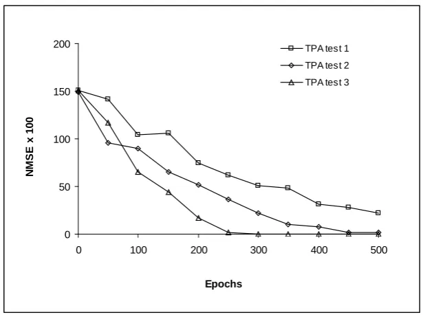
back-propagation algorithm for three neural network benchmark tasks. The principal strength of the tangent plane algorithm is that it does not require manually tuning a learning rate parameter, but instead automatically adjusts the learning rate to give the correct step size. The algorithm has been further modified to accept almost zero starting conditions with the expectation that only the minimum number of weight necessary will be activated during the training phase. The results show that the tangent plane algorithm gives improved generalization relative to the back-propagation algorithm, and that generalization is independent of network size. The limitations of the tangent plane algorithm are also identified

• A new sequential algorithm is developed referred to as the tangent plane

(4)

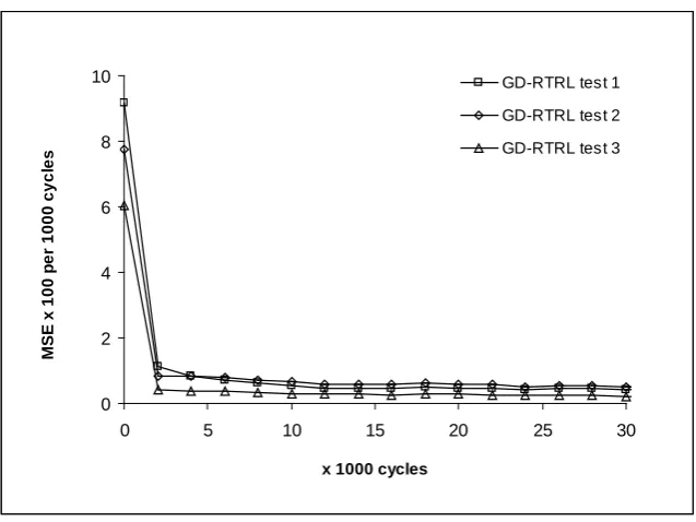
new algorithm is evaluated and compared with the original gradient descent real time recurrent learning (GD-RTRL) algorithm for two sequence recognition tasks. It is shown that using the new TPA-RTRL algorithm to train a fully recurrent neural network with feedback connections and context units is more stable than using the GD-RTRL algorithm, especially when the training data has been corrupted with a small amount of erroneous data.

• A new sequential algorithm referred to as the improved tangent plane

algorithm (iTPA) is developed to further improve the generalization performance of second tangent plane algorithm. This new algorithm is evaluated and compared with the original algorithm and the back-propagation algorithm for three neural network benchmark tasks. The results show that moving along tangent planes in a direction that encourages weight elimination improves generalization performance. The results also show that including a tendency to move laterally in random directions along tangent planes helps the algorithm to avoid local minima of the error landscape.

• A new batch algorithm referred to as the Gauss-Newton tangent plane

(5)

(6)

LIST OF FIGURES

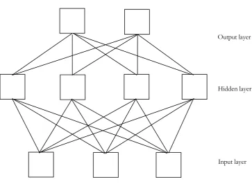
2.1 An example of a feedforward neural network with one hidden layer

12

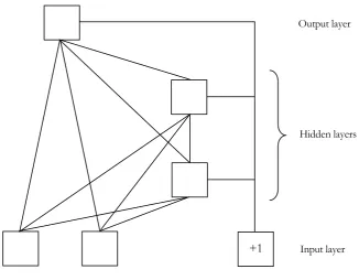
2.2 A cascade neural network with three input units, two hidden units and one output unit

13

2.3 An example of a recurrent neural network with one output layer 14 2.4 Error surface defined over two dimensional weight space 17 3.1 The structure of a multilayered feedforward neural network of

units {uj}

40

3.2 Movement from the present position in weight space to the foot of the perpendicular of a tangent plane

41

3.3 Typical convergence behaviour of the tangent plane algorithm on the 6-bit parity problem

52

3.4 Typical convergence behaviour of the backpropagation algorithm on the 6-bit parity problem

52

3.5 Typical convergence behaviour of the tangent plane algorithm with the teaching values randomised

53

3.6 Typical convergence behaviour of the backpropagation algorithm with the teaching values randomised

53

3.7 Typical generalization behaviour of the tangent plane algorithm on the hearta problem

58

3.8 Typical generalization behaviour of the backpropagation algorithm on the hearta problem

58

3.9 Typical generalization behaviour of the tangent plane algorithm on the cancer problem

60

3.10 Typical generalization behaviour of the backpropagation algorithm on the cancer problem

60

3.11 Importance coefficient histogram for the tangent plane algorithm (cancer problem).

63

3.12 Importance coefficient histogram for the backpropagation algorithm (cancer problem).

63

3.13 Importance coefficient histogram for the tangent plane algorithm (hearta problem).

64

3.14 Importance coefficient histogram for the backpropagation algorithm (hearta problem).

(11)

4.1 An example of a fully recurrent neural network with one output unit, one hidden unit, and two input units.

69

4.2 Movement from the present position to the foot of the perpendicular to the tangent plane of constraint surface

72

4.3 Typical convergence behaviour of the TPA-RTRL algorithm on the Xor problem with one unit trained to match the teaching signal

83

4.4 Typical convergence behaviour of the GD-RTRL algorithm on the Xor problem with one unit trained to match the teaching signal

83

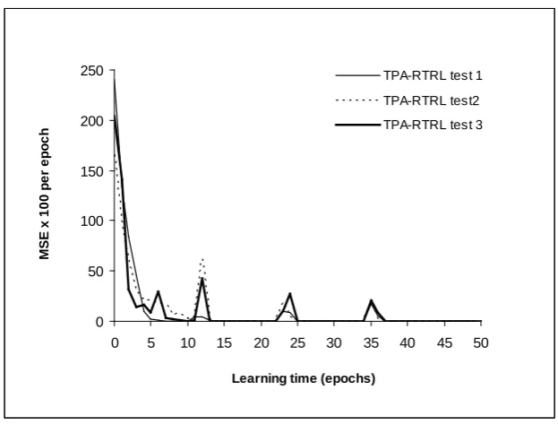
4.5 Typical learning curves of the TPA-RTRL algorithm on the simple sequence problem for a network with four processing units.

86

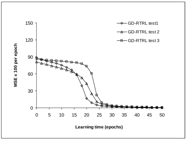
4.6 Typical learning curves of the GD-RTRL algorithm on the simple sequence problem for a network with four processing units.

86

4.7 Learning curves of the TPA-RTRL algorithm for a network with four processing units.

87

4.8 Learning curves of the GD-RTRL algorithm for a network with four processing units.

87

4.9 Typical convergence behaviour of the TPA-RTRL algorithm on the henon map time series prediction problem

89

4.10 Typical convergence behaviour of the GD-RTRL algorithm on the henon map time series prediction problem

89

5.1 The structure of a multilayered feedforward neural network of units {uj}

94

5.2 Movement from the present position a to the point e inclined at an

angle β to the tangent plane to the constraint surface

95

5.3 Typical generalization behaviour of the new iTPA algorithm on the two spiral problem

107

5.4 Typical generalization behaviour of the second tangent plane algorithm on the two spiral problem

107

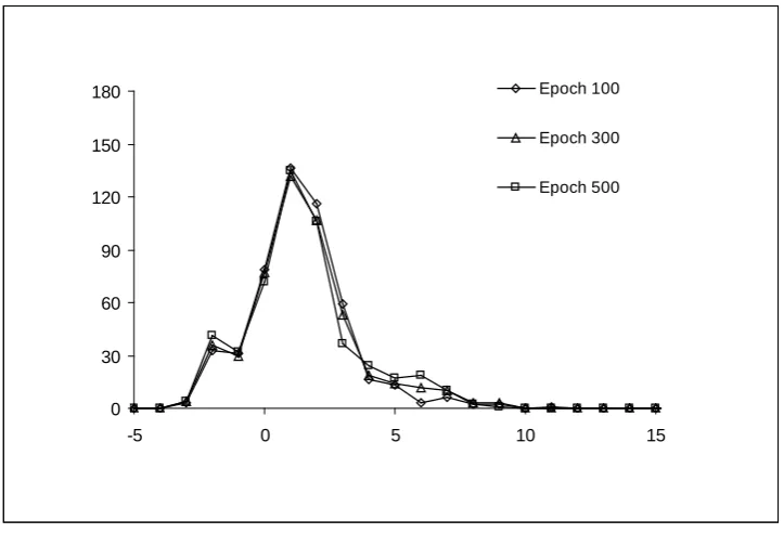
5.5 Importance coefficient histograms for the new iTPA algorithm (henon map problem)

109

5.6 Importance coefficient histograms for the second tangent plane algorithm (henon map problem).

109

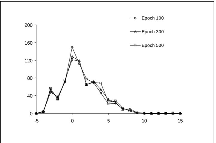
5.7 Importance coefficient histograms for the new iTPA algorithm (housing price problem).

111

5.8 Importance coefficient histograms for the second tangent plane algorithm (housing price problem).

(12)

6.1 Typical training curves generated by the batch-tangent plane algorithm on the additive function approximation problem

127

6.2 Typical training curves produced by the Rprop algorithm on the additive function approximation problem

127

6.3 Typical training curves produced by the batch-tangent plane algorithm on the breast cancer problem

129

6.4 Typical training curves produced by the Rprop algorithm on the breast cancer problem

129

7.1 Typical training and generalization curves produced by the ELM-tangent plane algorithm on the additive problem

147

7.2 Typical training and generalization curves produced by the Cascade algorithm on the additive problem

147

7.3 Typical training and generalization curves produced by the sequential training technique on the additive problem

148

7.4 The AIC at each training step for the ELM-TPA algorithm on the additive function problem

148

7.5 Plot of the model output generated by the ELM-tangent plane algorithm on the Henon map problem

150

7.6 Typical training and generalization curves produced by the ELM-tangent plane algorithm on the Henon map problem

150

7.7 Typical training and generalization curves produced by the Cascade algorithm on the Henon map problem

151

7.8 Typical training and generalization curves produced by the sequential training technique on the Henon map problem

151

7.9 Typical training and generalization curves produced by the ELM-tangent plane algorithm on the housing estimation problem

153

7.10 Typical training and generalization curves produced by the Cascade algorithm on the housing estimation problem

153

7.11 Training and generalization curves produced by the sequential training technique on the housing estimation problem

154

8.1 Comparison of classification accuracy for different categories on the GCM dataset

169

8.2 Comparison of classification accuracy for different categories on the GCM dataset

175

8.3 Comparison of classification errors on the DLBCL tumour class for each selected gene number

(13)

8.4 Comparison of classification errors on FL tumour class for each selected gene number

180

8.5 Comparison of classification errors on B-CLL tumour class for each selected gene number

180

LIST OF TABLES

3.1 Mean number of steps to converge for standard networks with different numbers of hidden units on 6-bit parity

50

3.2 Mean number of steps to converge on 6-bit parity for networks trained using fuzzy data

53

3.3 Training set error and testing set error for different sized networks with training terminated using early stopping

56

4.1 Mean number of steps to converge and number of successful trials for both algorithms on Xor problem

81

4.2 Weight matrix for Xor with one-cycle delay 81

4.3 Mean number of steps to converge and success rate on the simple sequence problem

84

4.4 Mean number of steps to converge and success rate on the simple sequence problem with n (%) of teaching values randomised

84

4.5 Number of epochs trained and test set error for the henon map time series prediction problem.

87

5.1 Classification error on the training set and test set, mean number of steps to converge, and number of success trials for different values of the weight sensitivity parameters

104

5.2 Results of a t-test comparing the mean test errors of the different algorithms.

110

6.1 Training set error and test set error for different size networks with training terminated using early stopping:

124

7.1 Training set error and test set error for three problem domains using: (a) ELM-TPA algorithm, (b) cascade algorithm, and (c) orthogonal sequential training technique

144

8.1 Partitioning of the GCM_training.res dataset into training and test samples.

(14)

8.2 Partitioning of the Lymphoma dataset into training and test samples.

159

8.3 Classification accuracy on the Lymphoma dataset for different algorithms

164

8.4 Classification accuracy (%) on the GCM dataset for different algorithms

165

8.5 Confusion matrix obtained for iTPA-OVA on the GCM problem. 168 8.6 Classification accuracy on the Lymphoma dataset for different

algorithms

170

8.7 Optimum values for the parameters of ELM-TPA for each selected gene number

170

8.8 Classification accuracy on the GCM dataset for different algorithms

171

8.9 Optimum values for the parameters of ELM-TPA for each selected gene number

172

8.10 Confusion matrix obtained for ELM-TPA on the GCM problem. 174 8.11 Results of a t-test comparing the mean test set errors for the two

algorithms.

(15)

Chapter 1 : Introduction

Chapter 1

INTRODUCTION

1.1 Motivation

(16)

time step ahead the correct response to an item of data received previously by the network [3,4,5]

(17)

The convergence speed of the tangent plane algorithm is no better than the standard back-propagation algorithm in small parsimonious networks where generalization is found to be best. In small networks with only a few synaptic weights, it seems that updating the weights by approaching tangent planes would be a very slow, as one big weight update might actually corrupt the whole of the network. In the batch mode of learning the weights are updated after the presentation of the entire dataset. Collecting all the gradient information together before the weights are updated helps to avoid the mutual interference of weight changes that could occur with large learning rates in the sequential (or online) learning. This makes the batch learning particularly suitable for training small neural networks. An alternative approach to batch learning might be to take smaller steps in weight space, the smaller steps averaging out the variations in the data so that the weights follow a more clearly defined trajectory in weight space. Unfortunately reducing the step size leads to slow adaptation of the weights so training speeds can be very slow. Furthermore iterative methods that take smaller steps are prone to being trapped in local minima of the error landscape. Therefore a new batch implementation of the tangent plane algorithm for training small parsimonious networks is investigated in this thesis

(18)

problems is to combine several binary classifiers, but this produces a heavy computational overhead. This means that fast and efficient algorithms are needed. The new sequential and batch tangent plane algorithms are particularly suitable for this purpose as they are very fast and avoid problems like overfitting and local minima. Therefore the new sequential and batch implementations of the tangent plane algorithm are applied to multi-category classification based on gene expression data

1.2 Objectives

The primary objectives of this research are to improve the convergence speed, stability and generalization of the tangent plane algorithm. More specifically, the objectives of this research can be summarised as follows

• Develop a new algorithm for fully recurrent neural networks targeted at improving the stability of the tangent plane algorithm. One example of where stability is an issue with the tangent plane algorithm is when the training data is contains a small amount of rogue data or errors. Therefore one objective of this thesis is to develop a new algorithm capable of accepting a small percentage of erroneous data in the training set and recovering quickly after it has been perturbed in this way

(19)

to develop a new algorithm giving improved generalization and evaluate its performance on non-trivial problems.

• Develop a new batch tangent plane algorithm for small parsimonious networks. The tangent plane algorithm is a fast method of training a neural network that does not require any parameters to be set manually to tune its performance. This is the principal strength of the tangent plane algorithm. However the tangent plane algorithm is no better than the back-propagation algorithm when applied to small economical networks where generalization is known to be best. Therefore another objective of this thesis is to develop a new algorithm for small economical networks capable of fast convergence and good generalization

• Apply the new sequential and batch algorithms developed in this thesis to multi-category classification tasks that have proven difficult for more conventional neural network techniques to solve. Cancer classification using gene expression data is considered a difficult task because of the high input dimension, and multi-category classification is far more difficult than binary classification. The classification accuracy of ANN is known to drop sharply as the number of classes increases. Therefore fast and efficient algorithms are needed that are capable of high classification accuracy

1.3 Major contributions of the thesis

The major contributions of this thesis can be summarised as follows. In the first part of this thesis, three new algorithms are developed to overcome the difficulties with the tangent plane algorithm

(20)

networks (FRNNs). This algorithm is evaluated for classification and time series prediction tasks. It is shown that the new TPA-RTRL algorithm is a very fast and stable method of training FRNN that recovers quickly when presented with items of erroneous data. This is because the FRNN recycles information over many time steps and thereby learns to predict the correct response a time step ahead, provided that an ordering of the input data exists.

• A new sequential algorithm referred to as the improved tangent plane algorithm (iTPA) is developed to further improve the generalization performance of the second tangent plane algorithm. This new algorithm is evaluated for pattern classification and function approximation tasks. The results show that implementing a weight elimination procedure into the geometry of the algorithm actually improves generalization performance by producing a separation of the active and inactive weights in the network. The results also show that including a tendency to move laterally in random directions along tangent planes helps the algorithm to avoid local minima of the error landscape.

(21)

In the later part of this thesis, the newly developed sequential and batch tangent plane algorithms are applied to real world classification tasks that have proven difficult for more conventional neural network techniques to solve. Multi-category cancer classification using gene expression profiles is a difficult task to solve due to the high dimensionality of the data. Traditionally this is done by combining binary classifiers in one-versus-one (OVO) or one-versus-all (OVA) schemes, which inevitably involves increasing the system complexity. Direct classification using artificial neural networks has been attempted but classification accuracy is known to drop sharply with increasing number of classes

• The new sequential algorithm is combined with a one-versus-all scheme for multi-classification using gene expression data. A modular network is used with each segment trained to discriminate one class from all others. The results show that the new scheme can produce classification accuracies comparable with other newly developed sequential learning algorithms, SANN and FGAP-RBF.

• The new batch algorithm is applied to multi-category micro-array gene expression data. One-of-c encoding is used with each output unit trained to discriminate one class from all others. Results show that the GN-TPA algorithm gives high classification accuracy comparable with SVM-OVO, which is the best SVM classifier.

1.4 Organisation of the thesis

(22)

discussed with strategies for improving generalization. Finally a brief overview of the bioinformatics area with an emphasis on gene expression data is discussed.

Chapter three investigates the convergence and generalization behaviour of the tangent plane algorithm. Comparative tests are performed using the standard back-propagation algorithm. The benchmark datasets used were N-bit parity, breast cancer and hearta. Two problems with the tangent plane algorithm were identified, namely slow convergence in small networks and instability when handling inexact data. Finally the differentiation and evolution of weight in networks trained by the tangent plane algorithm was investigated

In chapter four, a new algorithm referred to as TPA-RTRL is developed for fully recurrent neural networks targeted at improving the stability of the tangent plane algorithm. This new algorithm is similar to the GD-RTRL algorithm, differing from it in the treatment of the output unit and in the use of a global learning rate. Suggestions were made to improve the computational complexity of the new algorithm. Comparative tests are performed on the new TPA-RTRL algorithm and the gradient descent based GD-RTRL algorithm. The benchmark datasets used were pipelined Xor, the simple sequence problem, and the Henon map.

In chapter five, a new algorithm referred to as iTPA is developed to overcome the difficulty with the second tangent plane algorithm, namely the tendency of the algorithm to produce large network structures. Comparative tests were carried out on the new iTPA algorithm and the backpropagation algorithm. The benchmark datasets used were two spirals, Henon map and housing price.

(23)

instability due to the step size overshooting the error minimum and the computational complexity of the algorithm.

In chapter seven, the new GN-TPA algorithm is applied to the Extreme Learning Machine in order to overcome the difficulties with the algorithm. An additive technique for growing a neural network is used to improve the computational efficiency of the new algorithm. Comparative tests are performed using two additive procedures, cascade and the orthogonal sequential training technique. The benchmark datasets used were additive function, the Henon map and housing price.

In chapter eight, two multi-category classification problems using gene expression profiling are described, GCM and Lymphoma, together with a gene selection method for reducing the number of genes required for accurate cancer classification. Comparative tests were carried out using three sequential learning algorithms, iTPA, SANN, and FGAP-RBF, and three batch learning algorithms, GN-TPA, ELM, and SVM-OVO.

(24)

Chapter 2 : Literature review

Chapter 2

LITERATURE REVIEW

The back-propagation algorithm is a popular method for training feed-forward multilayered neural networks. It is easy to implement and computationally simple. The principal disadvantage of this learning method is its relatively slow rate of convergence in practical situations. It also requires manual tuning by appropriate choice of learning and momentum rate parameters, a process which is carried out by trial and error. Since one of the advantages of a neural network is the ease with which they may be applied to novel problems, it is essential to consider automated and robust learning methods with good performance on many classes of problems. In this chapter, we review some first order and second order optimization techniques known to accelerate convergence. Some of these methods require the adaptation of the parameters of the learning algorithm, whilst others use second order information about the error surface

(25)

In the cancer classification area, micro-array gene expression profiling has attracted more attention than conventional techniques such as microscopic histology and tumour morphology due to recent advances in micro-array technologies. Gene expression profiling allows for the monitoring of thousands of gene expression levels in any cell, cell line or tissue. Hence it provides more information and more reliable classification accuracy. There have been many classification methods used for cancer classification. However, there are some characteristics of gene expression data that make them difficult tasks. In this chapter we review some of the methods used for cancer classification with an emphasis on multi-category classification using gene expression data

2.1 Artificial neural networks

(26)

Fig 2.1. An example of a feed-forward neural network with one hidden layer

In feed-forward neural networks, the information flows in one direction from one layer to the next. The neurons in the input layer supply information, or activations, to the inputs of the neurons in the first hidden layer. The output signals of the neurons in the first hidden layer supply information, or activations, to the inputs of the neurons in the second hidden layer, and so on. Typically the neurons in each layer receive inputs from the output of the neurons in the preceding layer. Fig 2.1 illustrates the architecture of a multilayered feed-forward neural network (or multilayered perceptron). This network is referred to as a 3-4-2 network because it has 3 input neurons, 4 hidden neurons, and 2 output neurons. It is fully connected in the sense that every neuron in each layer is connected to every neuron in the next layer.

Output layer

Hidden layer

(27)

Another type of multilayered feed-forward structure has each neuron forming its own layer as illustrated in Fig 2.2. The cascaded neurons each receive an input from the neurons in the previous layers together with an input from the original network inputs, and pass their output to the neuron in the next layer. This cascade architecture was first proposed by Fahlman and Lebiere [7], and has been used successfully with many neural network problems that have proven very difficult for the standard back-propagation algorithm to solve [8,9,16,17]

+1

Output layer

Hidden layers

Input layer

Fig 2.2. Cascade network architecture with three input units, two hidden units

(28)

Fig 2.3. An example of a recurrent neural network with one layer. The function z-1 is the unit delay operator whose output is delayed with respect to the input by one time step i.e. z−1

[ ]

x( )_jk =x(_jk−1) where x_j is the jth input and k the time step.

Recurrent neural networks on the other hand distinguish themselves by comprising at least one feedback loop. For example, a recurrent neural network may consist of a single layer of neurons with each neuron feeding its output signal back to the inputs of the other neurons. The presence of a feedback loop has a profound effect on the learning capacity as well as its performance [6]. The feedback loops can involve the use of unit delay operators that can result in a non-linear dynamic behaviour. Thus, recurrent neural networks find greatest use in time series prediction problems [3,4,5].

z-1 _z-1

(29)

2.2 Learning in artificial neural networks

A neural network learns about its environment by an adaptive process whereby a series of adjustments are made to the synaptic connections, or weights, and bias levels. Ideally, the network becomes more knowledgeable about its environment after each adaptive process. We define the learning process in the context of neural networks as follows [18]:

Learning is a process by which the free parameters of a neural network are adapted

through a process of stimulation by the environment in which the network is

embedded. The type of learning is determined by the manner in which the parameter

changes take place.

(30)

2.2.1 First order methods and variants

The method of steepest descent is an iterative procedure for obtaining the values of the parameters that minimise the error (or cost) function. When applied to a neural network, this is equivalent to finding the values of the synaptic weights that connect the network units together. Geometrically, the function specifies an error surface defined over weight space. At each iteration of the steepest descent procedure, the weights are adjusted in the direction in which the error function decreases most rapidly. This direction is given by the negative gradient of the error function at the current point in weight space. The magnitude of the modification is proportional the magnitude of the error gradient. The procedure can be written

( )

( ) ( )n ji n k n

ji

w

∂

−

=

∆

η

ε

(2.1)

where ∆w_ji is the change to the weight w_ji that regulates the connection from unit

i

u

to u_j,

η

is a positive constant called the learning rate, ε_k is the error function to

be minimized, and

n

the time step. There are two main error functions, one is sum of square errors (SSE) and the other is the relative entropy function [19]

(31)

illustrated in Fig. 2.4. The error surface is drawn topographically using constant error contours. The current weight vector is given by

w

( )n . Since the error surface is

steeper along the

w

₂( )n weight dimension than the

w

₁( )n dimension, the derivative along this weight dimension will be larger.

Fig 2.4. Error surface defined over two dimensional weight space

A simple method of reducing the oscillations due to a large learning rate is to modify equation (2.1) as follows

( ) ( ) ( ) ( ) ji t k n 0 t t 1 n ji ji n k n ji w w w w ∂ ∂ − = ∆ + ∂ ∂ − = ∆

∑

=

− _η _α ε

α ε

η (2.2)

where

α

is a positive constant called the momentum term, and

∆

w

(_jin−1) the change

applied to weight w_ji during the

(

n−1

)

th step.

1

w

2

w

( ) ( )n 2 n k

w

∂

ε

( )

( )n 1 n k

w

∂

∂ε

(32)

According to Jacobs [20], the back-propagation algorithm with momentum is an exponentially weighted sum of the current and past partial derivatives of the error function. For this algorithm to be convergent, the momentum constant must be restricted to the range 0≤

α

<1. Note that when

α

is zero the back-propagation algorithm operates without momentum. When consecutive derivatives of a weight have the same sign, the weight

w

_ji is adjusted by a large amount, and when

consecutive derivatives possess opposite signs, this sum is adjusted by a small amount as above. Thus, the inclusion of a momentum will either accelerate learning in a downhill direction, or have a stabilizing effect in directions that oscillate. The momentum term may also have the benefit of preventing the learning process from terminating in a shallow minimum of the error surface.

In view of the poor performance of the back-propagation steepest descent algorithm, it has been suggested that the value of the learning rate η be adapted according to the contours of the error function [20,21,22,23]. The learning rate η is then treated as another factor to alter the step size of the weight change on the error surface. At present a number of strategies for adapting the learning rate can be found in the literature. These strategies can be divided into two broad classes; global and local learning rate adaptation. Global learning rate adaptation involves finding the proper value for the learning rate [21,24,25,26,27]. Local learning rate adaptation involves using independent learning rates for each adjustable weight in the network [20,28,29,30,31,32]. Two examples are discussed below

(33)

current position to the zero error plane. This is equivalent using a tangential hyper-plane to locally approximate the error function. Let

ε

_k represent the error caused by

some particular pattern, so that

ε

_k is a function of the weights

w

. Linearising the

dependence of

ε

_k on

w

about some operating point

w

( )n

' k

ε

(

w

) =

ε

_k

(

w

( )n

) + (

w

−

w

( )n

)

.

∇

ε

_k

(

w

( )n

)

(2.3)

where ∇

ε

_k = (

∂

ε

_k

∂

w

_j,_i ),

∀

j

,

i

represents the gradient vector, and

a .

b

represents the inner product of vectors

a

and b. We wish to find a zero of the error function

ε

_k, so

0 =

ε

k

(

( )n

w

) + (

w

−

w

( )n

)

.

∇

ε

k

(

( )n

w

)

(2.4)

Let

∆

w

( )n

=

w

(n+1)

−

w

( )n . From the method of steepest descent, the weights are

adjusted according to

∆

w

( )n

=

−

η

∇

ε

_k( )n , so the value of

η

that sets the linearised

error

ε

'_k = 0 is given by

( ) ( )

( )

(

)

2

i , j

ji n k

n k n

w

∑

∂

=

ε

η

(2.5)

where

j

,

i

range over all the weight indices. For practical reasons it is necessary to

define an upper limit

η

_max for a single step. There may also be some error surfaces

that never reach the zero plane. For these surfaces, a small constant value

ε

_off is

(34)

Unfortunately it is likely to result in very big updates that may corrupt the whole network in one step. This strategy also can’t handle very big datasets where some wrongly classified training examples might exist.

In the second example, each individual weight has a corresponding learning rate that is allowed to vary over time. The Rprop (resilient back-propagation) algorithm [28] differs from other first order techniques in that the individual step-sizes ∆_ji are

independent of the magnitude of the partial derivatives ∂

ε

_k ∂w_ji. For each weight

ji

w

, an individual step-size

∆

_ji is adjusted according to

( ) ( ) ( ) ( ) ( ) ( ) ( ) ( )











∆

<

∂

∆

>

∂

∆

=

∆

− − − − − − +

otherwise

w

if

w

if

n ji ji n k ji n k n ji ji n k ji n k n ji n ji 1 1 1 1 1

0

ε

η

ε

η

(2.6)

After adjusting the step-sizes, the weight updates

∆

w

_ji are determined. The weight

update rule can be written

( ) ( ) ( )n ji ji n k n ji w sgn

w _∆

      ∂ ∂ − =

∆

ε

(2.7)

(35)

signs of the current and previous derivatives. When the signs of successive derivatives are opposite, this means that the algorithm has jumped over a minimum and that the step size is too large. On the other hand if two successive signs are equal, then the step size is not big enough and could be increased. Finally, local back-tracking is usually applied to those weights when a change in the sign of the corresponding derivatives are detected

(36)

2.2.2 Second-order optimization techniques

In the sequential mode of learning, weight updating is performed after the presentation of each training example. This mode of learning is also referred to as on-line, pattern, and stochastic mode. In the batch mode of learning, weight updating is performed after the presentation of all the training examples. There are several advantages in favour of each type of learning mode as outlined by Battiti [37]. One of the reasons in favour of sequential learning is that it possesses a degree of randomness that may help in escaping from a local minimum. The fact that many large datasets contain redundant data has also been cited in favour of sequential learning, because many of the contributions to the gradient are similar, so waiting to collect all the gradient information together can be wasteful. On the other hand, collecting all the gradient information together before the weights are updated can help to avoid the mutual interference of weight changes that occur with large learning rates. Sequential methods may because of their degree of randomness, miss a perfectly good local minimum. Even if the training data is redundant, sequential methods may be slow in comparison to batch methods that use second-order information. Some second-order batch techniques show superior performance with respect to the standard back-propagation algorithm on problems with a limited number of weights (< 100), especially if high precision mappings are required.

Newton’s method can be considered as the basic locally convergent method using second-order information. It is based on using a second order Taylor expansion of the error function

ε

_k about the current operating point

w

k

ε

(

w+∆w

)

≈

ε

k

(

w

) +

∇ ∆w T k

ε

+

∆w ∇ k∆w 2 T 2

1

ε

(37)

and solving for the step ∆w that brings

w

to a point where the gradient is zero. This corresponds to solving the following linear system

k k

2

ε

∆

=

−

∇

ε

∇

w

(2.9)

Generally speaking, Newton’s method converges quickly to a solution and does not exhibit the zigzagging behaviour that characterises the steepest descent method. The main problems that can arise with Newton’s method is when the Hessian

∇

2

ε

_k is

not positive definite (i.e. the directional derivative ∆ ∇2 ∆ <0 w

wT

ε

_k ), or when the Hessian is singular or ill-conditioned. If the Hessian is not positive definite, there exists directions

∆

w

of negative curvature that would suggest an infinite number of steps to minimise the error function. This behaviour is not uncommon in neural networks: in some cases large steps push units into saturation resulting in very small second order derivatives.

When the Hessian matrix is not positive definite and well conditioned, Newton’s method cannot be used without modifications. This can be explained by examining the eigenvalues of the Hessian. Writing the Hessian using a spectral decomposition, we have

∑

=

Λ

=

∇

n

i

T i i ii T

k

1 2

u

U

Λ

ε

(2.10)

where Λ is a diagonal matrix whose diagonal elements

Λ

_ii are the eigenvalues of

(38)

of numerical problems. If one of the eigenvalues is negative, the error function does not have a minimum because large movements in the direction of the corresponding eigenvector decrease the error value to arbitrary negative values.

A recommended strategy for changing the Hessian in order to avoid these difficulties is that of summing it to a diagonal matrix of the form

µ

_k

I

so that

∇

2

ε +

_k

µ

_k

I

is

positive definite and well-conditioned. A proper value for

µ

_k can be found using the modified Cholesky factorisation found in Gill et al [38]. The Cholesky factors of a positive definite matrix can be considered as a sort of square root of the matrix. The original matrix is expressed as the product

L

D

L

T, where L is a lower triangular matrix with 1’s on the leading diagonal, and

D

is a diagonal matrix with positive diagonal elements. Taking the square root of the diagonal elements using them to form the matrix _D12_{, the original matrix can be written as}_L_D12_D12_LT = _Lˆ _LˆT_{, where}

Lˆ is a general lower triangular matrix. If the original matrix is not positive definite, the factorization can be modified in order to obtain factors

D

with all diagonal elements positive. The factorization corresponds to the original factors of the Hessian, and differing from it by adding a diagonal matrix with non-negative elements.

If the error function to be minimised is the sum of error squares,

∑

=

= m

p p

k ₁

e

2 2

1

ε

,

where

e

_p is the error of the pth input pattern, learning a set of examples consists of

(39)

Let the error signal

e

_p be a function of the weight vector

w

∈

R

n. The gradient and

Hessian matrix of

ε

_k are given by

e

J

_eT

m

p

p p

k

=

∇

=

∇

∑

=1

e

ε

(2.11) and

[

]

S

J

+

=

∇

+

∇

=

∇

∑

= e T e m p p p

k

e

1 2 T p p 2

e

ε

(2.12)

where

J

_e is the Jacobian matrix [

∂

e

∂

w

_j ],

e

is a vector of errors

e

_p, and S is that

part of the Hessian containing the second derivatives of

e

, that is, =

∑

∇

p

e

p

e

p

2

S .

For small residual problems (i.e. small values of

e

_p), the second order part S is negligible, and Newton’s method can be written

=

∆w - [J_eTJ_e

]

−1J_eTe (2.13)

It can be shown that this step is completely equivalent to minimizing the error obtained using a first order Taylor expansion of the error, e'. The updated weight vector is then defined by

{

' '

}

2

1

min

e

w

T

=

(2.14)

(40)

method has quadratic or second order convergence as the minimum on the error surface is approached. Meyer [39] has shown that the convergence of the Gauss-Newton method is superlinear (i.e. ||e( )t+1 ||

/

||e( )t ||→0,

t

→

∞

) whenever S →0, otherwise it is only first order.

The only problem that can arise with equation (2.12) is the Jacobian matrix

J

_e being

rank deficient, and hence J_eTJ_e is singular. The Levenberg-Marquardt (LM) method [40] incorporates a technique for dealing with a rank deficient

J

_e, and is effective for

small residual problems. In this method a diagonal matrix

µ

I is added to J_eTJ_e, where

µ

is a small positive constant and I the unit matrix. When

µ

=0, ∆w is given by [

J

_eT

J

_e

]

−1

J

Te

e

. As

µ

→∞, the effect of the term

µ

I increasingly

dominates that of

J

_eT

J

_e so that ∆w →

µ

−1J_eTe, which represents an infinitesimal step in the steepest descent direction.

(41)

2.3 Generalization capabilities of artificial neural networks

A neural network is said to generalize well when the output computed by the network is correct for test data not used in training the network. Here it is assumed that the test data is drawn from the same population as the training data. If the learning process is viewed as a curve fitting problem then the neural network itself may be considered as a non-linear input-output mapping. Such a viewpoint then permits us to look on generalization simply as the effect of good non-linear interpolation. Neural networks can perform useful interpolation because multilayer neurons with continuous activation functions lead to output functions that are also continuous [43].

A neural network that generalizes well will produce a correct input-output mapping even when the test data is slightly different from the examples used to train the network. However, when a neural network learns too many input-output examples the network may end up memorising the training data. It may do so by finding a feature in the training data such as noise that is not present in the underlying function. Such a phenomenon is referred to as overfitting or overtraining. When a network is overtrained it loses its ability to generalize between similar input-output patterns

Good generalization performance in a neural network is influenced by a number of different factors; the size of the training set, the size of the network and the complexity of the problem at hand [6].

(42)

• A neural network that is too small may fail to learn the underlying function, that is, it will underfit the training data. However, a network that is too large may tend to overfit the training data and thus generalize poorly to new data. Thus, there is a trade-off between underfitting and overfitting.

• The underlying function must be sufficiently smooth. A network can learn functions with a finite number of discontinuities but not totally chaotic or random functions.

(43)

2.3.1 Constructive techniques

Constructive methods start out with a small network and then add new units and connections until the network can represent the required function. Perhaps the most notable example of constructive methods is the Cascade Correlation algorithm proposed by Fahlman and Lebiere [7]. The cascade correlation algorithm increases the size of the network by adding new units and layers. There are two distinctive features to the cascade correlation algorithm. First, the cascade architecture. This means that all the hidden units are added to the network one at a time, each on a separate hidden layer. The cascade structure leads to the creation of powerful high-order feature detectors and to very deep networks. Second, the objective function used to train the new hidden units. For each new hidden unit, the cascade-correlation process aims to maximize the magnitude of the correlation between the hidden units output and the residual network error signal. The cascade-correlation architecture thus has several advantages over conventional back-propagation; it learns very quickly, the network determines its own size, it preserves its structure even if the training set changes, it does not require back-propagating error signals, and only one layer of weights are trained at a time.

(44)

from existing centres and if the output error is large. If the input pattern does not pass the criteria for novelty, then no hidden unit is added and the network is trained using the OLS method. In [47] a new method for RBF networks named GAP-RBF was described which adds and prunes hidden units based on a simple estimate of the significance of centres. The significance of a unit is the error that results from removing that unit from the network over all inputs seen so far. Results for GAP-RBF show it can achieve a smaller network realized by RAN, and that it achieves higher classification accuracies and better generalization.

(45)

2.3.2 Network pruning techniques

(46)

2.3.3 Other techniques for improving generalization

Overfitting can also be avoided by reducing the complexity of the data in the input data set. A technique called Principal Component Analysis (PCA) can be used to project the input vectors onto a vector space whose basis is described by the eigenvectors of an input correlation matrix. The reduction is achieved by choosing the principal components of the input vectors that have the largest variance. There are many examples of architectures performing PCA in the literature [54,55,56,57,58]. For example, the well-known generalized hebbian algorithm (GHA) proposed by Sanger [56], and the adaptive principal component extractor (APEX) proposed by Kung and Diamantaras [57]. Both are extensions of Oja’s principal component neuron [55]. Fiori [58] applied these algorithms together with the new ψ-APEX to 20 datasets containing 5,000 samples. The results show that ψ-APEX and GHA give the best results when the eigenvalues of the correlation matrix are spread wide apart, otherwise they are the same.

(47)

results. He proposed the use of a new error measure based on the median of the absolute error. The median tends to reduce the effects of a few erroneous results on the overall sample average.

(48)

2.4 Multi-category classification using gene expression data

Bioinformatics is defined as the storage and manipulation of biological information [63]. Luscombe [64] defines bioinformatics as conceptualising biology in terms of molecules and applying informatics techniques to understand and organise the information associated with these molecules on a large scale. One aspect of bioinformatics is the analysis of biological data. This involves gene identification and prediction, gene structure prediction, and the investigation of macro structures such as secondary and tertiary protein structures, and examining protein geometries using distance and angle measures. Another aspect of bioinformatics is the biological data itself. One property of biological data is the extremely large amount. For example a DNA sequence of genes comprises strings of four base letters, each gene 1,000 bases long. The GenBank [65] repository holds more than 12.5 million bases in 115 million entries.

(49)

training sample size and number of genes results in a very sparse input space, which makes accurate classification very difficult. Third, most of the genes are irrelevant to cancer classification, and simply add back-ground noise to any analysis carried out.

There has been a number of classification methods used for cancer classification both from statistical and machine learning. These methods include k-nearest neighbour [66,72], linear discriminant analysis [68,70,72], and support vector machines [73,74,75]. Nearest neighbour methods are based on some distance function of a pair of patterns, such as the Euclidean distance. The k-nearest neighbour rule proceeds as follows. For each pattern in the test set, find the k-nearest patterns in the training set, and predict the class of the pattern by majority vote, that is choose the class that is most common among the k-nearest neighbours. Linear discriminant analysis is a method that finds the linear combinations of features which best separate two or more classes. The resulting combination can be used as a linear classifier or, more commonly, for dimensionality reduction. Fisher linear discriminant analysis is based on finding linear combinations of pattern vectors with large ratios of between-class to within-between-class sum of squares. This measure is in some sense a measure of the signal to noise ratio for the class labelling. One of the first applications of discriminant methods to gene expression data was the weighted voting scheme [70]. In this method a sample is assigned to a particular class according to the weighted distance between it and the nearest class mean vector. Support vector machines map the input space into a higher dimensional feature space so that the data is linearly separable into two classes. This separation is achieved by constraining the Euclidean norm of the weight vector.

(50)

drop off sharply as the number of classes increases. Ramaswamy et al [74] applied an SVM algorithm for the analysis of gene expression data on 14 different tumours in the GCM dataset. For a c-category classification problem, c binary classifiers were used each to discriminate one class from all others. This method has potential drawbacks when there is considerable overlap between classes in pattern space. The results are very promising in relation to k-nearest neighbour and weighted voting methods. Yeang et al [69] have made a comparison of three binary classification methods, k-nearest neighbour, weighted voting and support vector machines. Three combinatory schemes were used, one-versus-all, one-versus-one, and hierarchical partitioning. The results show that all the support vector machines produced the best results when all the genes were used. For the k-nearest neighbour and weighted voting methods, one-versus-one tended to outperform one-versus-all when a fixed number of genes were used. Dudoit et al [72] made a comparison of linear discriminant methods, nearest neighbour classifiers, decision trees and aggregation methods. Three datasets were used, lymphoma, leukaemia, and NCI60. The results show that the k-nearest neighbour method and diagonal linear discriminant method had the lowest test set errors, and that the Fisher discriminant method had the highest test set error. Stratnikov et al [78] presents a comprehensive evaluation of several multi-category classification methods including SVM, k-nearest neighbour, weighted voting and a back-propagation neural network. The study used nine multi-category datasets and two binary datasets; GCM dataset, brain tumour dataset, leukaemia dataset, MLL dataset, lung cancer dataset, SRBCT dataset, prostrate tumour dataset and DLBCL dataset. The results show that SVM classifiers were the best performers with and without gene selection, and that weighted voting and decision tree methods were the worst; the back-propagation neural network ranked in the middle.

(51)

(52)

Chapter 3 : Comprehensive evaluation of the tangent plane algorithm

Chapter 3

COMPREHENSIVE EVALUATION OF THE TANGENT PLANE ALGORITHM

In Lee [14], an algorithm is described for supervised learning in multilayered feed-forward neural networks. This second tangent plane algorithm uses the target values of the training data to define a surface in the weight space of the network. The weights are updated by moving to the tangent plane to this surface. It differs to more conventional gradient descent based learning methods by accepting almost zero initial conditions with the expectation that only the minimum number of weights will be activated. It has been shown to give improved generalization and significantly faster convergence relative to the standard back-propagation algorithm on benchmark classification problems.

(53)

3.1 Description of the tangent plane algorithm

A neural network must have the right size for good generalization. Networks that are too small cannot fit the required function, whereas networks that are too large are prone to overfitting [82]. There are several approaches to determine the correct size for a network. In Lee [14] a method was described that grows the weights from almost zero initial conditions in the expectation that only the necessary number of weights would be activated. Lee used the first tangent plane algorithm [2] as a starting point, for instead of determining a single direction to move on in weight space, it determines a plane of suitable points to move to. The first tangent plane algorithm is a fast method of training a feed-forward neural network. It avoids inappropriate step sizes by treating each training value as a constraint that defines a surface in weight space. The weights are then adjusted by moving from the current position to the tangent plane to this surface. The second tangent plane algorithm adjusts the weights by moving from the current position to a point close to the foot of the perpendicular, but displaced somewhat in the direction away from the origin. This directional component of movement helps to push the network weights away from the origin where the convergence speed of the tangent plane algorithm, and other steepest descent methods, is known to be very slow [2]. In the region of weight space close to the origin the axis defined by the weight from the constant output bias is very nearly perpendicular to all the constraint surfaces. Thus the tangent plane algorithm gives movement up and down this axis satisfying the constraints on the weights by adjusting this weight only.

(54)

3.1.1 Derivation of the tangent plane algorithm

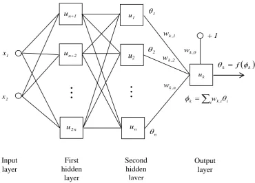
The basic structure of a feed-forward neural network is shown in Fig 3.1. It consists of an input layer of units that supply information, or activations, to the inputs of units in the first hidden layer. These in turn supply activations to inputs of units in the next layer, and so on. Typically the units in each layer receive inputs from the output of the units in the preceding layer. Let w_ji denote the weight between unit

u

_i and u_j.

j

φ

and

θ

_j will be the input and output of u_j, so that

θ

j = f (

φ

j) and

φ

j

=

∑

_i

w

ji

θ

i

for some monotonic function f .

Let

u

_k be trained to mimic the target value

y

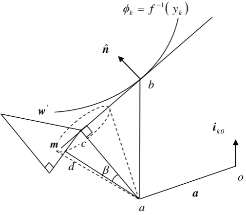
_k. The tangent plane algorithm adjusts

the weights by moving at an angle

β

to the perpendicular from

a

to the tangent

plane to the surface

φ

_k = f−1

( )

y_k , taken at a point where a line dropped from

a

Fig. 3.1. The structure of a feed-forward neural network

Input layer First hidden layer Output layer Second hidden layer k u 1 u 1 , k w 0 , k w

( )

k

k f φ

θ = n u n 2 u 2 , k w n , k w

∑

=

i k.i i

k w θ

φ 1 + 1 θ 1 x 2

x



(55)

and parallel to the axis defined by the output unit’s bias weight

w

_k₀ meets this surface (see Fig. 3.2).

Let

=

∑

i , j ji ' ji

w

i

a

, where i_ji is a unit vector in the direction of the w_ji axis. Use the equation −

( )

=

+

∑

_≠

0 i ki i 0 k k 1

w

y

f

θ

to find a value, w"_k₀, for the bias weight

0 k

w

from the values w_ji of the other weights, so that the surface

φ

_k = f−1

( )

y_k

contains the point = +

∑

_≠

0 , k i , j ji ' ji 0 k " 0 k w

w i i

b . Now, if we use the equation

( )

∑

_≠ −

=

+

0 i i ' ki " 0 k k 1

w

y

f

θ

and −

( )

=

+

∑

_≠

0 i i ' ki ' 0 k k 1

w

f

θ

, and note that b differs

from

a

only in the value of

w

_k₀, we get

(

)

( )

(

k

)

k0

1 k 1 0 k ' 0 k " 0 k

f

y

f

w

i

a

b

θ

− −

−

=

−

=

−

(3.1)

Fig. 3.2. Movement from the present position a to the foot of the perpendicular to the tangent plane of constraint surface φ_k= f−1

( )

y_k to position d

o

c

( )

k 1 k f y

(56)

Let nˆ be the unit normal to the surface at b, so

n

ˆ

=

∇

φ

_k

∇

φ

_k . The length of the perpendicular from

a

to the tangent plane at b is

(

b

−

a

)

.

n

ˆ

. If

c

is the foot of the perpendicular from

a

to the tangent plane at b,

( )

(

)

( )

k k k k k k k k k k k k

f

y

f

.

f

y

f

φ

θ

φ

θ

∇

−

=

∇

−

=

−

− − − − 1 1 0 1 1

i

a

c

(3.2)

The vector parallel to the tangent plane and directed away from origin at

a

is

(

a

.

n

)

n

a

m

=

−

ˆ

. Thus, if

d

∈

R

n is the point of intersection with the tangent plane

of a line from

a

inclined at angle

β

to the perpendicular, then

(

) (

)

(

c a

)

m m a c a c c d a d − + − = − + − = −

β

tan (3.3)

Let

δ

= f −1

( )

y_k − f −1

( )

θ

_k be the error in the input to final unit. Hence, using equations (3.2) and (3.3), we obtain

(57)

So, to adjust a given weight

w

_ji

    ∂ ∂ ∂ ∂ ×     ∇ − ∇ + ∂ ∂ ∇ = ∆

∑

ji k lm lm k lm k ji k ji k k ji w w w w tan w w

φ

β

φ

δ

φ

δ

φ

2 2

1 1 1 m (3.5) where 2 ji k i ,

j l,m lm

k lm 2 k ji 2 w w w 1

w _

  ∂ ∂           ∂ ∂ ∇ −

=

∑

φ

m

The term ∂φ_k ∂w_ji is the partial derivative of the net input to the output unit. This

derivative is evaluated at point w" on the constraint surface, not at the current position

w

' in weight space. The

Improved sequential and batch learning in neural networks using the tangent plane algorithm