A Strain Range Dependent Cyclic Plasticity Model

Please cite this article as: E. Khademia, G.H. Majzoobi, N. Bonora, A Strain Range Dependent Cyclic Plasticity Model, International Journal of Engineering (IJE), TRANSACTIONS B: Applications Vol. 30, No. 2, (February 2017) 321-329

International Journal of Engineering

A Strain Range Dependent Cyclic Plasticity Model

E. Khademia*a_{, G.H. Majzoobi}b_{, N. Bonora}c

a _{Department of Robotics, Hamedan University of Technology, Hamedan, Iran}

b _{Department of Mechanical Engineering, Faculty of Engineering, Bu-Ali Sina University, Hamedan, Iran} c _{Department of Civil and Mechanical Engineering, University of Cassino and Southern Lazio, 03043 Cassino, Italy}

P A P E R I N F O

Paper history: Received 03 March 2016

Received in revised form 09 December 2016 Accepted 22 January 2017

Keywords:

Simulation Hysteresis Loop Cyclic Plasticity Model Neural Network

A B S T R A C T

Hysteresis loop curves are highly important for numerical simulations of materials deformation under cyclic loadings. The models mainly take account of only the tensile half of the stabilized cycle in hysteresis loop for identification of the constants which don’t vary with accumulation of plastic strain and strain range of the hysteresis loop. This approach may be quite erroneous particularly if the mean stress is not small and the effect of isotropic hardening is large. A strain dependent cyclic plasticity model which considers the variation of material constants versus strain range and accumulation of plastic strain has been proposed and experimentally investigated by the authors. In this paper it is proved that their proposed model is accurate for simulating all cycles of the hysteresis loop regardless of the strain range of the test. It is shown in this work that artificial neural network (ANN) model, if designed and trained properly, can be used for interpolating and extrapolating the experimental data. The results of this work are compared with two well-known cyclic plasticity models. The results also indicate that there is a remarkable agreement between the proposed model and ANN within and outside the strain ranges used in the experiments.

doi: 10.5829/idosi.ije.2017.30.02b.20

NOMENCLATURE X Back stress tensor

a, ar _{Isotropic hardening constants (Pa) z, z}r _{Isotropic hardening constants}

𝑏 Isotropic hardening parameter Greek Symbols

𝐶 Kinematic hardening parameter (Pa) ν Poisson’s ratio

E Elasticity modulus 𝜎 Stress tensor

f Yield function 𝜎0 Initial yield stress (Pa)

𝐽2 Second stress invariant (Pa) 𝜀𝑃 Plastic strain tensor

N Flow direction tensor  Kinematic hardening parameter

p Accumulated plastic strain Subscripts

q Strain amplitude mono Monotonic loading

Q Isotropic hardening parameter (Pa) QR, bR Isotropic hardening

𝑅̂(𝑝) Isotropic hardening (Pa) αC, βC, α, β Kinematic hardening

1. INTRODUCTION1

The nonlinear behavior of material under cyclic loading has extensively been investigated over the past decades [1-4]. The behavior of most of materials is very complicated on one hand and most of cyclic material models are pure empirical and the identification of their

1_{*Corresponding Author’s Email:e.khademi@hut.ac.ir (E. Khademi)}

which are normally determined by simple techniques such as trial and error. These types of techniques are tedious and time consuming on one hand and the accuracy of results is dependent on the skill and experience of researcher on the other hand. Therefore, most of the models are not widely used for simulation, design and analysis. One of the most recent techniques for identification of the constants is optimization. This technique, however, involves a large amount of computations. In order to reduce the computational efforts, an automated system for optimization of material parameters is presented [9, 10].

Along with the efforts for improving the material models, attempts have also been made to simulate material behavior directly from experimental data. This will assist the users to avoid the deficiencies involved in material models. One of the most recent techniques which are widely employed for predicting the behavior of materials under cyclic loadings is artificial neural network (ANN). The interpolating and extrapolating capabilities of this model, for a properly trained network, may be exploited for prediction of material behavior for test condition within and outside the ranges used in the experiments. This will reduce the cost and save the time for conducting tedious, costly and time consuming tests. Lefik and Schrefler [11] used experimental results of transverse cyclic loading of superconducting cable for training ANN and examined the model for interpolation within the input data. Janezic et al. [12] presented an approach based on the neural network for describing the variation of stress-strain curve under cyclic loading with the temperature, specimen diameter and strain amplitude. The prediction of low cycle fatigue life of a particular steel alloy at various temperatures was studied by Mathew et al. [13]. Purintrapiban and Corley [14] used ANN model for describing the state of the auto-correlated process in cyclic condition for condition monitoring process. Tomasella et al. [15] showed that experimental tests for estimating the life of a material under cyclic loading can partially be replaced by artificial neural network model. In another work for accurate simulating of cyclic plasticity by ANN for a metal, Furukawa and Hoffman [16] used two separate neural networks, one for back stress and the other for isotropic hardening evolution. Although, ANN has widely been used for simulation of cyclic behavior of materials by many authors, no attention has been paid to possibility of the use of ANN for describing accurate evolution of stress-stress curve in the hysteresis loop of a material under fully reversed loading.

In this paper, material parameters determined by Khademi et al. [17] using an automated system for fully annealed 99.99% pure copper, will be used for simulating the material response under cyclic loading at different strain amplitudes. The experimental data will also be used for identification of material parameters for

Ohno and Wang [4] and Rahman et al. nonlinear models [9]. Finally, a comparison is made between the results of the proposed model, experimental results and Ohno-Wang and Rahman et al. models.

Artificial neural network will also be employed for prediction of cyclic behavior of material using the test data obtained in this investigation. Four sets of input data will be used for training ANN in a way that the best agreement between the experiment and ANN prediction is obtained. In order to avoid overtraining, a new method for incorporating the full cycle of hysteresis loop into the neural network will be presented in this work. Once the ANN is trained for the strain range used in the experiments in this work, the cyclic behavior of material outside the experimental strain range is determined by interpolation and extrapolation of the data used for ANN training.

2. MATERIAL MODELS

High ductile and strain hardened material such as pure copper shows intense nonlinear behavior under cyclic loading. Therefore, the simulation of the hysteresis curves of this material can reveal the accuracy of the material model. In order to simulate the material behavior under fully reversed strain control cyclic loading, the material parameters obtained from experiment by Khademi et al. [17] for fully annealed 99.99% pure copper are used for three different models. The main model is proposed by the authors of this work. The results are compared with two other models proposed by Rahman et al. and Ohno and Wang.

2. 1. The Proposed Model by Khademi et al. Khademi et al. [17] proposed a set of explicit corrector equations for solving the following nonlinear constitutive equations:

   

2 0 ˆ 0

fJ σ X  R p  (1)

p_

ε N (2)

4

1 2

3 m P

m

m m

C  p



 





X ε X (3)

  2





1

ˆ i _{1 exp} i

R R

i

R p Q b p



 





Khademi et al. [17] showed that material parameters evolve with p and q. In the case of isotropic hardening, material parameters given by Equation (4) are defined in terms of plastic strain and strain amplitude as follows:





1 exp 1,2

i i i

R QR QR

Q a _  z q_ i (5)





exp 1,2

i i i

R bR bR

In Equation (3) four back stresses are considered to simulate the kinematic hardening behavior in which third back stress considered linear (𝛾3_{= 0) and also} slope of this line is assumed constant, 𝐶3_{= 385(𝑀𝑃𝑎).} Other three back stresses evolve with the accumulated plastic strain as follows:









m m m

D D

D    p DC m (7)

where, 𝛼𝐷𝑚and 𝛽𝐷𝑚 are material parameters and vary with strain amplitude as follows:

exp( ) , & 1, 2, 4

m m m m

D aD bD kDq D C m

       (8)

exp( ) , & 1, 2, 4

m m m m

D aD bD kDq D C m

       (9)

where, 𝑎𝛼𝐷𝑚, 𝑏𝛼𝐷𝑚, 𝑘𝛼𝐷𝑚, 𝑎𝛽𝐷𝑚, 𝑏𝛽𝐷 𝑚 and 𝑘𝛽𝐷𝑚 are material constants. Finally,

, 1, 2

exp( ) , 1, 4

, 2, 4

m m m m

H H H

H a m

H e f g q H b m

H k m



 

 

     

  



(10)

All Material constants as obtained by Khademi et al. [17] are given in Table 1. In this work, the constants given in Table 1 are incorporated in a finite element code and the cyclic stress-strain curves predicted by finite element method are compared with those measured from the experiments.

In the finite element code developed in this work, a fully implicit method is used for calculating stress recovery and tangent modulus at each load increment.

TABLE 1. New material constants [17]

The commercial finite element code MSC.MARC 2010 R1 was used for simulating material behavior with the constants of the proposed material model through the user subroutine HYPELA2.F. This routine is used for obtaining stiffness tangent matrix and the stress tensor at each increment. The values of variables such as the accumulated plastic strain and the back stresses are stored as state variables for subsequent calculations. The procedure used for implementing the model in the subroutine of the FEM code is summarized as:

1. Readthe material constants from the input file

2. Call state variables

3. Calculate elastic stiffness matrix and trial stress

4. Calculate trial yield function, trial

f

IF trial 0

f  THEN:

4-1- Calculate initial values for iterative scheme

4-2- Calculate correctors

4-3- Update variables with adding correctors to state variables

4-4- If residual functions are smaller than the Tolerance, CONTINUE

ELSE repeat 4-2 and 4-3

5. Calculate consistent tangent matrix

6. Calculate stress, elastic and plastic strain isotropic hardening and back stresses

7. SAVE new variables into state variables

Trial stress is calculated by assuming an elastic regime for each increment. The simulations are performed using the material constants given in Table 1 (as the input for FEM code). Rectangular four-node element with 1mm×1mm size and axisymmetric analysis is considered for the numerical study. One side of the element is fixed and fully reversed displacement with various amplitudes is applied to the opposite side. Therefore, strain control condition with different strain ranges can be simulated. The predicted hysteresis loop for 1%, and 3% strain ranges are depicted in Figures 1 and 2, respectively in which the experimental hysteresis loop is also plotted for comparison with the proposed model. As the figures indicate, the proposed model can predict material response under cyclic loading from the beginning to the saturated cycle regardless of the strain range. The results of the proposed model are compared with two basically different cyclic plasticity models including Ohno-Wang multilinear model and Rahman et al. nonlinear model. The models are briefly described in the next sections. In the model introduced by Krishna et al. [6], material constants are determined from cyclic test on a single specimen under different strain amplitudes. However, in the present work, one specimen is used for one strain amplitude. Therefore, it is not basically right to compare the results of this work with those reported by Krishna et al. [6]. On the other hand, although Zhang and Jiang [18] used single specimen for each strain range (similar to the present work) they did not consider isotropic hardening effect.

E(GPa) 0(MPa) 

115 21 0.3

1 4 mono C 1 4

mono

  1,2,4

C

a b1,2,4C k1,2,4C

1,2,4 C

a b1,2,4C k1,2,4C

2.06e4 3614.3 6.30e5 2.70e6 184 3 1.5 -136

1454.9 15.8 2.70e4 1.45e5 139 5.3 5.7 150

385 0 1.20e4 1.20e4 -110 3 13.5 130

608.8 73.4

1,2,4

a b1,2,4 k1,2,4 gb2,4

1,2 a

e 1,2

a

f 1,2

a

g 1,4

b f

3.25e4 2.8e4 161 189 3.7 19 211 1.1

400 8370 233 -415 9 16 138 115

350 240 -120

1,4 b

g 1,4

b

e 2,4

b

e 2,4

b

f a4 b2 k1

-161 2.6 50 342 5.5 3e3 30

160 1 14 4e-3

QR

a a_bR r

QR

a r

bR

a zQR zbR r QR

z r

bR z

It should be noted that elastic properties and isotropic hardening evolution are the same for all models considered in this investigation.

2. 2. Rahman et al. Model Rahman et al. model [9] uses four rules Chaboche model for evolution of kinematic hardening. This model was initially proposed by Bari and Hassan [2] for finding material constants. However, Rahman et al. [9] divided tensile half cycle into four segments in each of which a back stress term was dominant. They also introduced physical meanings for Cm and m _{for the first time and developed an}

automated program for finding the most appropriate segment for each back stress with the best agreement with the experimental data. In this model, only the tensile half cycle of the stabilized cycle is considered for finding the material parameters and the identified parameters remain constant for the other cycles. The strain amplitude for the hysteresis curve which is used for identification of parameters is assumed reasonably large to ensure that all back stresses (except the third one) get stabilized within the strain range [2].

-0.50 -0.25 0.25 0.50

-160 -80 0 80 160

Experiment Psoposed model

(MPa)



Figure 1. Experimental hysteresis loop and proposed model results for 1% of strain range

-1.5 -1.0 -0.5 0.5 1.0 1.5

-200 -150 -100 -50 0 50 100 150 200

Experiment Psoposed model

  (MPa)

Figure 2. Experimental hysteresis loop and proposed model results for 3% of strain range

Therefore, hysteresis loop with the largest strain range is used for determining the material parameter in this model. The material constants computed for the strain range of 4% are given in the appendix.

2. 3. Ohno-wang Model Ohno and Wang [4] introduced a multilinear model by dividing stabilized tensile half cycle into several segments and assuming linear hardening for each segment. Kinematic hardening rule for each linear part was similar to Armstrong and Frederick [1]. However, Ohno and Wang [4] used a step function in their model in which each decomposed hardening rule evolves linearly with the slope of Cm

until approaches m m

C  and remains constant

afterward. Obviously, by increasing the number of hardening rules a better agreement with the experimental curve will be expected. Bari and Hassan [2] have argued that the best performance of this model is achieved when the strain range for obtaining the material parameters is assumed reasonably large. Therefore, 14 back stresses were considered for the model and the constants were obtained from the stabilized tensile half cycle for the strain range of 4%. The constants obtained using this model are provided in the appendix.

material constants given in Table 1. Therefore, it can be concluded that evolutions of Cm and m _{are valid}

within the entire strain ranges used in this investigation. In order to demonstrate the degrees of accuracy of the models discussed above more clearly, the evolutions of the stress amplitude, a, and the mean stress, m, of

each cycle, as predicted by the models and obtained from the experiments, versus accumulated plastic strain are compared in Figures 5 and 6 for strain ranges of 1.5% and 4%, respectively. As the figures suggest, for the stress amplitudes, there is excellent agreement between the proposed model and the experiments so that, except for few points, the prediction of the proposed model and the experimental data coincide with a high degree of accuracy.

Therefore, the proposed model is able to accurately predict the maximum and minimum stress in each cycle. This may be attributed to the fact that the proposed model has been developed by taking account of the entire stress-strain curve in the hysteresis loop for all strain ranges.

It may also be due to the formulations of material constants as described by Khademi et al. [17].

-2 -1 0 1 2

-200 -150 -100 -50 0 50 100 150 200

q=2% Stabilized cycle

Experiment Proposed model Rahman et al.(2005) Ohno-Wang(1993)





(

M

Pa

)

Figure 3. A comparison between various models and experimental data for stabilized cycle and the strain amplitude of 2%

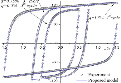
-1.5 -1.0 -0.5 0.0 0.5 1.0 1.5

-120 -60 0 60 120

q=0.75% 3rd cycle

q=1.5% 1stcycle



q=0.5% 5th cycle

Experiment Proposed model

Figure 4. A comparison between proposed model and experimental data for different cycles and different strain amplitude

0 10 20 30 40 50

0 30 60 90 120 150 180

-5



(

MPa

)

p

q=0.75

_a(Experiment)

_m(Experiment)

Proposed model

Rahman et al.(2005)

Ohno-Wang(1993)

Figure 5. A comparison between the numerical and experimental evolutions of stress mean and amplitude with accumulated plastic strain for strain range of 1.5%

0 10 20 30 40 50

-50 40 80 120 160 200

p



(

MPa

)

q=2

_a(Experiment)

_m(Experiment)

Proposed model

Rahman et al.(2005)

Ohno-Wang(1993)

Figure 6. A comparison between the numerical and experimental evolutions of stress mean and amplitude with accumulated plastic strain for strain range of 4%

The results of the other two models are almost similar except for small strain ranges for which the models are slightly different. The difference, however, decreases with the increase of strain range. The interesting point is that for stress amplitude, the gap between the proposed model and the other two models becomes wider for smaller strain ranges. As the strain range increases, the models come closer to each other so that for the strain range of 4%, they nearly coincide. Another interesting point is that the difference between the proposed model and the other two models reduces for higher plastic strain.

parameters are assumed to be the same for all cycles. The relative convergence of the models for amplitude stress at high plastic strains is due to determination of the material parameters from stabilized cycle of the largest strain rang.

3. INTERPOLATION AND EXTRAPOLATION USING ANN

Artificial neural networks (ANN) consist of computational pattern based on the recognition between input parameters and solution of a problem. The biological neural system and artificial neural networks have similar characteristics such as pattern identification and capability of parallel computing. Also, the performance of the neurons is the basis of both systems. Unlike the models which make use of physical theories and consider predefined relations between inputs and outputs, ANN learns the trend between input data and solutions during the training phase. Therefore, the strength of the network sensibly depends on the number of data and relevance between them that are used in training phase. ANN can be used to predict the solution within the range of data as well as extrapolation beyond the range. The architecture of ANN consists of an input layer, an output layer and one or more hidden layers, which are located between input and output layers. This architecture is called multilayer network. Each neuron in the input layer connects to all the neurons in the hidden layers and each neuron in the hidden layers connects to all the neurons in the output layer but the neurons of a layer are not connected to each other. Synapse is the connection between two neurons and has a strength or weight that affects the output signal of the neuron. All the weights on the input side of a neuron accumulate and the output signal is calculated using a transfer function.

Neurons of the hidden layer receive signals from neurons in the input layer and send signals to the neurons of the output layer. Finally, the output signals are sent by neurons of the output layer. This kind of feeding is called feed forward method. In the training phase, the ANN output is compared with the real output (which is measured by experiments) and error is sent back to the neurons of the hidden layer to update the weights for minimizing the error. The performance of ANN is represented by error function which is introduced as the sum of squares of the difference between desired and predicted outputs. Back-propagation algorithm updates network weights in which error function decreases most rapidly utilizing gradient descent method as learning function. All the data should be normalized to balance the importance of each data during training phase.

In this work, a multilayer feed forward artificial neural network with hyperbolic tangent sigmoid as

transfer function, Levenberg-Marquardt

back-propagation for training, gradient descent weight for learning function and mean squared error for performance function are utilized and tested in the MATLAB package. Considering all the hysteresis loops with 1%, 1.5%, 3% and 4% strain ranges, four different types of experimental data are used for training the neural network, (1) the maximum stress versus accumulated plastic strain of the hysteresis curve; (2) the minimum stress versus accumulated plastic strain of the hysteresis curve; (3) the stress-strain curve of the first cycle and (4) the stress-strain curve of the stabilized cycle. Since there are four strain ranges, for each type of experimental data four individual input data can be obtained. For cases 1 and 2, one hidden layer with two neurons are used in the ANN in which input data is the accumulated plastic strain and target is the maximum and the minimum stress, respectively. Since, for cases 3 and 4 the relation between input data (strain) and output (stress) is highly nonlinear, three hidden layers are used in which four, six and eight neurons are considered in the first, second and the last hidden layer, respectively. Figure 7 shows ability of the designed ANN in learning evolution of maximum stress versus accumulated plastic strain for different strain ranges.

For the cyclic stress-strain curve, a new method for training the ANN is proposed. In this method, a cycle denoted by ABC in Figure 8 is replaced by an expanded cycle indicated by A’B’C’ in the same figure.

This is to enforce a unique correspondence between stress and strain in the stress-strain cycle. For the constructing the A’B’C’ root, AB path is considered first and strain magnitude of point A is subtracted from all points of the path. So, the entire path shifts to the left of stress axis. Then, by inversing the strain sign, path A’B’ is generated. Finally, the path BC is shifted to the right in which point B of this path is superimposed on B’ of the previously constructed A’B’ path.

0 10 20 30 40 50

0 40 80 120 160 200

p



(

MPa

)

Maximum stress of cycles (ANN) Experiment,q=0.5%

Experiment,q=0.75% Experiment,q=1.5% Experiment,q=2%

-2 -1 1 2 3 4 5 6 7 8

-150 -100 -50 0 50 100

150 C C'

B' A'

B





(

M

Pa

)

Experiment q=2% Experiment-extracted strain

Predicted- ANN A

Figure 8. The experimental initial cycle, the modified cycle used for training the ANN and predicted curve by neural network for 2% strain range

It must be mentioned that in the original cycle, each point on the strain axes corresponds to two values of stresses, a tensile and a compressive stress. This problem can be avoided by modifying the cycle as explained above. Figure 8 illustrates the first cycle (experimental) of the hysteresis loop for the strain range of 4%, the modified cycle used for training ANN model and the predicted curve by neural network. This figure shows an excellent agreement between experimental data and predicted curve from neural network. This could partly be due to the use of enough input data and neurons for training ANN.

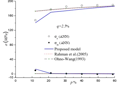
Finally, by restoring the expanded cycle, the normal cyclic stress-strain curve is obtained. Having achieved a good performance in the training phase, ANN will be used for accurate interpolation and extrapolation within and outside the strain ranges, respectively. For this purpose, the strain ranges of 2% and 5% are selected for interpolation and extrapolation, respectively. Figure 9 shows variation of amplitude of stress,a, and mean

stress,_m, versus the accumulated plastic strain for the cyclic loading with the strain range of 2%. As it can be seen, the proposed model has a good agreement with the curves predicted by neural network from the first cycle, where the models proposed by Rahman et al. and Ohno-Wang fail to completely simulate material response. Another feature of Figure 9 is that the proposed model can simulate all the cycles in the hysteresis loop with a reasonable accuracy. The results shown in Figure 10 for the strain range of 5% (q=2.5%) show exactly the same trends as described for the strain range of 2% (q=1%). However, proposed model has an excellent agreement with the results of ANN in the low and high accumulated plastic strain for the evolution of stress amplitude, but similar to other two models cannot simulate well the predicted curve among the range. The difference can presumably be due to either inadequacy of the number of material constants used in the exponential function to express the evolution of m

C and

m

 or the exponential function itself which may have not

been a right function to describe the evolution. Nevertheless, beyond the strain ranges of experimental data, the proposed model can simulate the initial and the last cycles more accurately than the other cycles in the hysteresis curve. Except for the initial cycles, the mean stress predicted by Rahman et al. and Ohno-Wang models is close to that predicted by the proposed model and obtained from the experiment.

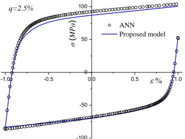
In order to study the ability of the proposed model in simulating the cyclic stress-strain curve within and outside the experimental strain range, a comparison between the proposed model, ANN and other two models has been made for the first and stabilized cycles with the strain ranges of 2% and 5%, respectively. The interpolated first cycle of hysteresis loop for 2% strain range is illustrated in Figure 11. As the figure indicates, the proposed model shows a good agreement with neural network interpolation for both compressive and tensile half cycles. Again, this confirms the accuracy of the proposed model and the procedure employed for identification of material parameter. The extrapolated stabilized cycle of hysteresis loop for 5% strain range is presented in Figure 12.

Figure 9. Comparison between ANN interpolation and other models for variation of stress amplitude and mean stress versus accumulated plastic strain

-1000 -100 10 20 30 40 50 60

0 40 80 120 160 200

q=2.5

p



(

M

Pa

)

_a _m Proposed model

Rahman et al.(2005)

Ohno-Wang(1993)

Figure 10. Comparison between ANN extrapolation and other models for variation of stress amplitude and mean stress versus accumulated plastic strain

0 10 20 30 40 50

0 30 60 90 120 150 180

-10

q=1

p



(

M

Pa

)

_a

_m

Proposed model

Rahman et al.(2005)

-1.0 -0.5 0.0 0.5 1.0

-100 -50 0 50 100

q=2.5%





(

M

Pa

)

ANN Proposed model

Figure 11. ANN interpolation and proposed model for first cycle of stress-strain curve

-2.50 -1.25 0 1.25 2.50

-200 -150 -100 -50 0 50 100 150 200

q=2.5%

ANN

Proposed model Rahman et al.(2005) Ohno-Wang(1993)





(

M

Pa

)

Figure 12. ANN extrapolation with other models for stabilized cycle of stress-strain curve

As the figure suggests, the proposed model shows a better agreement with ANN than the other models for both compressive and tensile half cycles. Figure 12 also indicates that the difference between the proposed model, ANN and the other two models is not significant. Again, the reason is that the other two models are more accurate for the stabilized cycle of hysteresis curve at and in the vicinity of the reference strain range (the strain range for which material parameters are obtained).

4. CONCLUDING REMARKS

In this work, strain dependent cyclic plasticity model proposed by Khademi, Majzoobi, Bonora and Gentile [17] was numerically investigated. Therefore, the proposed material model was implemented in the commercial finite element code MSC. MARC and the numerical results were validated by comparing with experimental data. In addition, interpolation and extrapolation of experiments were predicted by artificial neural network. The numerical results of the proposed

model were compared with the results of Rahman et al. and Ohno-Wang models as well as ANN. However, the proposed model is a complementary work for and modification into the models suggested by the pioneers such as Rahman et al. and Ohno-Wang who indeed paved the ground for the present investigations. The following conclusions may be derived in this paper:

1. Material parameters for Rahman et al. and Ohno-Wang models are obtained from the stabilized cycle of hysteresis loop for the largest strain range. These parameters don’t vary with accumulation of plastic strain and strain range of hysteresis loop. Therefore, the models can simulate only the cycles close to the stabilized cycle of a hysteresis curve for a strain range close to the range used for parameter identification. This approach yields a linear evolution of maximum and minimum stress versus accumulated plastic strain which is not usually seen in experiment.

2- The proposed model which considers the variation of material constants versus strain range and accumulation of plastic strain can predict accurately all cycles of the hysteresis loop regardless of the strain range of the test. This model can simulate compressive half cycles in the hysteresis loop from the first to the last cycle. The other models lack this feature which is highly important for simulation of material cyclic behavior.

3- If artificial neural network model trained properly, it can predict experimental data well and consequently the model can be used for interpolating and extrapolating the experimental data.

4- There is a remarkable agreement between the proposed model and ANN within and beyond the stain ranges of the tests. This suggests that the proposed model can perfectly predict material response within and beyond the strain range.

5. APPENDIX

Rahman et al. model constants:

1 4

C = 448177.5, 18336.1, 385, 121086.3

1 4

  _{= 39200.9, 346.5, 0, 1875.6} Ohno-wang model constants:

1 14

C = 142759, 26862, 4289, 7042, 8009, 2485, 1852, 3400, 2958, 1740, 2268, 2163, 1370, 362

1 14

  _{= 3081, 1583, 1303, 1094, 908, 728, 655, 585, 461,} 401.7, 342, 238, 137.9, 29.2

6. REFERENCES

2. Bari, S. and Hassan, T., "Anatomy of coupled constitutive models for ratcheting simulation", International Journal of Plasticity, Vol. 16, No. 3, (2000), 381-409.

3. Chaboche, J.-L., "Time-independent constitutive theories for cyclic plasticity", International Journal of Plasticity, Vol. 2, No. 2, (1986), 149-188.

4. Ohno, N. and Wang, J.-D., "Kinematic hardening rules with critical state of dynamic recovery, part i: Formulation and basic features for ratchetting behavior", International Journal of Plasticity, Vol. 9, No. 3, (1993), 375-390.

5. Chaboche, J.-L., "On some modifications of kinematic hardening to improve the description of ratchetting effects",

International Journal of Plasticity, Vol. 7, No. 7, (1991), 661-678.

6. Krishna, S., Hassan, T., Naceur, I.B., Sai, K. and Cailletaud, G., "Macro versus micro-scale constitutive models in simulating proportional and nonproportional cyclic and ratcheting responses of stainless steel 304", International Journal of Plasticity, Vol. 25, No. 10, (2009), 1910-1949.

7. Collin, J.-M., Parenteau, T., Mauvoisin, G. and Pilvin, P., "Material parameters identification using experimental continuous spherical indentation for cyclic hardening",

Computational Materials Science, Vol. 46, No. 2, (2009), 333-338.

8. Feng, X.-T. and Yang, C., "Genetic evolution of nonlinear material constitutive models", Computer Methods in Applied Mechanics and Engineering, Vol. 190, No. 45, (2001), 5957-5973.

9. Rahman, S.M., Hassan, T. and Ranjithan, S.R., "Automated parameter determination of advanced constitutive models", in ASME Pressure Vessels and Piping Conference, American Society of Mechanical Engineers. (2005), 261-272.

10. Yun, G.J. and Shang, S., "A self-optimizing inverse analysis method for estimation of cyclic elasto-plasticity model parameters", International Journal of Plasticity, Vol. 27, No. 4, (2011), 576-595.

11. Lefik, M. and Schrefler, B., "One-dimensional model of cable-in-conduit superconductors under cyclic loading using artificial neural networks", Fusion Engineering and Design, Vol. 60, No. 2, (2002), 105-117.

12. Janezic, M., Klemenc, J. and Fajdiga, M., "A neural-network approach to describe the scatter of cyclic stress–strain curves",

Materials & Design, Vol. 31, No. 1, (2010), 438-448.

13. Mathew, M., Kim, D.W. and Ryu, W.-S., "A neural network model to predict low cycle fatigue life of nitrogen-alloyed 316l stainless steel", Materials Science and Engineering: A, Vol. 474, No. 1, (2008), 247-253.

14. Purintrapiban, U. and Corley, H., "Neural networks for detecting cyclic behavior in autocorrelated process", Computers & Industrial Engineering, Vol. 62, No. 4, (2012), 1093-1108.

15. Tomasella, A., El Dsoki, C., Hanselka, H. and Kaufmann, H., "A computational estimation of cyclic material properties using artificial neural networks", Procedia Engineering, Vol. 10, (2011), 439-445.

16. Furukawa, T. and Hoffman, M., "Accurate cyclic plastic analysis using a neural network material model", Engineering analysis with Boundary Elements, Vol. 28, No. 3, (2004), 195-204. 17. Khademi, E., Majzoobi, G.H., Bonora, N. and Gentile, D.,

"Experimental modeling of strain-dependent cyclic plasticity for prediction of hysteresis curve", The Journal of Strain Analysis for Engineering Design, Vol. 50, No. 5, (2015), 314-324.

18. Zhang, J. and Jiang, Y., "Constitutive modeling of cyclic plasticity deformation of a pure polycrystalline copper",

International Journal of Plasticity, Vol. 24, No. 10, (2008), 1890-1915.

A Strain Range Dependent Cyclic Plasticity Model

E. Khademiaa_{, G.H. Majzoobi}b_{, N. Bonora}c

a _{Department of Robotics, Hamedan University of Technology, Hamedan, Iran}

b _{Department of Mechanical Engineering, Faculty of Engineering, Bu-Ali Sina University, Hamedan, Iran} c _{Department of Civil and Mechanical Engineering, University of Cassino and Southern Lazio, Cassino, Italy}

P A P E R I N F O

Paper history: Received 03 March 2016

Received in revised form 09 December 2016 Accepted 22 January 2017

Keywords:

Simulation Hysteresis Loop Cyclic Plasticity Model Neural Network

ديكچ ه

یاه لدم بلغا .دنراد ییازسب تیمها یا هخرچ یاهراب تحت داوم لکش رییغت یددع یزاس هیبش یارب دنامسپ هقلح یاه ینحنم رظن رد هدام لدم یاه تباث نییعت یارب ار صخشم شنرک هزاب کی رد دنامسپ هقلح زا رادیاپ هخرچ یششک شخب طقف هدش هئارا

اب اه تباث نیا دوش یم ضرف هک دنریگ یم یم یقاب رییغت نودب دنامسپ هقلح شنرک هزاب رییغت و ناسموم شنرک عمجت شیازفا

یدایز یاطخ اب تسا دایز درگناسمه یگدنوش تخس ای و تسین کچوک شنت نیگنایم هک یماگنه ًاصوصخم ضرف نیا .دننام ددعتم تاشیامزآ هیاپ رب و قیقحت نیا ناگدنسیون طسوت هک نیا هب هجوت اب .تسا هارمه ناسموم هدام لدم کی

هتسباو یا هخرچ

نیا رد ،دنا هداد هئارا دنبای یم رییغت هتفای عمجت ناسموم شنرک نازیم زین و شنرک هزاب اب هدام لدم یاه تباث نآ رد هک شنرک هب شنرک یاه هزاب رد دنامسپ هقلح یاه هخرچ مامت یزاس هیبش یارب یداهنشیپ هدام لدم هک دوش یم هداد ناشن هلاقم زا توافتم

و یحارط تسرد یعونصم یبصع هکبش رگا هک دش دهاوخ هداد ناشن هلاقم نیا رد نینچمه .دشاب یم رادروخرب یبسانم تقد لدم ود اب قیقحت نیا جیاتن .دومن هدافتسا یشیامزآ یاه هداد یبای نورب و یباینایم روظنم هب نآ زا ناوت یم دوش هداد شزومآ ناسموم -اقم فورعم یا هخرچ یعونصم یبصع هکبش و یداهنشیپ لدم نایم یبوخ قابطنا هک دنهد یم ناشن جیاتن .تسا هدش هسی

.دراد دوجو اه نآ زا جراخ رد نینچمه و یشیامزآ شنرک یاه هزاب نیب رد