Acceleration of Bluff Body Calculation Using Mdgrape-2

169

ACCELERATION OF BLUFF BODY CALCULATION

USING MDGRAPE-2

T. K. Sheel

MEMA, University Catholique de Louvain, Batiment Euler, 4 Avenue Goerges Lemaitre 1348 Louvain-La-Neuve, Belgium

[email protected] - [email protected]

S. Obi

Department of Mechanical Engineering, Keio University, Tokyo, Japan

(Received: August 18, 2009 – Accepted in Revised Form: October 5, 2009)

Abstract Bluff body calculation was accelerated by using a special-purpose computer,

MDGRAPE-2, that was exclusively designed for molecular dynamics simulations. The three main issues were solved regarding the implementation of the MDGRAPE-2 on vortex methods. These issues were the efficient calculation of the Biot-Savart and stretching equation, the optimization of the table domain, and the round-off error caused by the partially single precision calculation in the MDGRAPE-2. Finally this technique was applied to calculation of flow around a circular cylinder. The drag and lift coefficient was investigated to check the validity of the proposed method.

Keywords Vortex Method, MDGRAPE-2, Bluff Body, Drag and Lift Coefficient

ﻩﺪﻴﻜﭼ

هﮋﻳو ﺮﺗﻮﻴﭙﻣﺎﻛ ﻚﻳ زا هدﺎﻔﺘﺳا ﺎﺑ ﻲﻟﺎﺧ ﻪﻧﺪﺑ ﻪﺒﺳﺎﺤﻣ ﻖﻴﻘﺤﺗ ﻦﻳا رد )

MDGRAPE-2 (

ياﺮﺑ ًاﺮﺼﺤﻨﻣ ﻪﻛ

ﻪﻴﺒﺷ يزﺎﺳ ﺪﺷ ﻊﻳﺮﺴﺗ ﺖﺳا هﺪﺷ ﻲﺣاﺮﻃ ﻲﻟﻮﻜﻟﻮﻣ ﻚﻴﻣﺎﻨﻳد يﺎﻫ .

ياﺮﺟا ﻪﺑ طﻮﺑﺮﻣ ﻢﻬﻣ ﻪﻟﺎﺴﻣ ﻪﺳ MDGRAPE-2

رد

شور ﺪﺷ ﻞﺣ ﻲﺑادﺮﮔ يﺎﻫ .

ﺪﻣآرﺎﻛ ﻪﺒﺳﺎﺤﻣ ﻪﻟﺎﺴﻣ ﻪﺳ ﻦﻳا Biot-Sarvat

يﺎﻄﺧ و لوﺪﺟ هزﻮﺣ يزﺎﺳ ﻪﻨﻴﻬﺑ ،ﺶﺸﻛ ﻪﻟدﺎﻌﻣ و

ﻨﻣ ﻖﻴﻗد ﻪﺒﺳﺎﺤﻣ زا ﻞﺻﺎﺣ ندﺮﻛ دﺮﮔ رد ﻲﺋﺰﺟ دﺮﻘ

MDGRAPE-2 دﻮﺑ

. رد نﺎﻳﺮﺟ ﻪﺒﺳﺎﺤﻣ ياﺮﺑ ﻚﻴﻨﻜﺗ ﻦﻳا ﺖﻳﺎﻬﻧ رد

ﺖﻓر رﺎﻛ ﻪﺑ روﺪﻣ ﻪﻧاﻮﺘﺳا ﻚﻳ فاﺮﻃا .

راﺮﻗ ﻲﺳرﺮﺑ درﻮﻣ يدﺎﻬﻨﺸﻴﭘ لﺪﻣ رﺎﺒﺘﻋا لﺮﺘﻨﻛ ياﺮﺑ ندﺮﻛ ﺪﻨﻠﺑ و ﺶﺸﻛ ﺐﻳﺮﺿ

ﺖﻓﺮﮔ .

1. INTRODUCTION

Flow around a circular cylinder is a fundamental fluid mechanics problem of practical importance. It has potential relevance to a large number of practical applications such as submarines, off shore structures, bridge piers, pipelines etc. The laminar and turbulent unsteady viscous flow behind a circular cylinder has been the subject of numerous experimental and numerical studies, especially from the hydrodynamics point of view. External flows past objects have been studied extensively because of their many practical applications. For example, airfoils are made into streamline shapes in order to increase the lifts, and at the same time, reducing the aerodynamic drags exerted on the wings. On the other hand, flow past a blunt body,

such as a circular cylinder, usually experiences boundary layer separation and very strong flow oscillations in the wake region behind the body. In certain Reynolds number range, a periodic flow motion will develop in the wake as a result of boundary layer vortices being shed alternatively from either side of the cylinder. This regular pattern of vortices in the wake is called a Karman vortex street. It creates an oscillating flow at a discrete frequency that is correlated to the Reynolds number of the flow. The periodic nature of the vortex shedding phenomenon can sometimes lead to unwanted structural vibrations, especially when the shedding frequency matches one of the resonant frequencies of the structure.

vortical flows related with problems in a wide range of industries, because they consist of simple algorithm based on physics of flow [1;4]. Leonard [8] summarized the basic algorithm and example of its applications.

The vortex methods have made remarkable advancements in the past decade, but still face numerous challenges, especially involving the high computation cost.

There has always been a strong relationship between progress in vortex methods and advancements in acceleration techniques that utilize this method. When the classical vortex methods became popular nearly 30 years ago, the calculation cost of the N-body solver was O(N2) for N particles. Due to this enormous calculation cost, the intention at that time was not to fully resolve the high Reynolds number fluid flow, but to somewhat mimic the dominant vortex dynamics using discrete vortex elements.

One of the main difficulties of vortex methods to be accepted in the mainstream of computational fluid dynamics is the numerical complexity of calculating the velocity using the Biot-Savart law, which is in fact analogous to an "N-body problem" and hence requires O(N2) operations for N vortex elements.

There are two techniques to reduce the force calculation cost of an N-body simulation: hardware and software techniques. In the hardware, there are two techniques, one is a parallel computer and the other is a special-purpose computer. To accelerate the vortex methods calculation, parallel computation has been widely used in previous studies [9;11-14]. Even though accelerate the calculation significantly; there are some difficulties to use parallel computations for longer calculations. It has limitations with parallelization according to hardware specifications. The memory bandwidth is a big problem to calculate for large number of vortex elements, which required special consideration. Power consumption and heat dissipation interrupt the longer time calculations. These problems are becoming serious for advanced scientific computation. Shortcomings of parallel computers, the special-purpose approach can solve parallelization limit thoroughly. It has relaxed power consumption according to hardware specification.

The special-purpose computer has been used in

the present calculations to avoid the difficulties of parallel computations with higher speed. Hardware accelerators such as MD-GRAPE [6], and MDGRAPE-2 [16] have been developed and successfully applied to MD simulations [16]. Yatsuyanagi [18] has used MDGRAPE-2 to accelerate the velocity calculation of Biot-Savart integral equation for the simulation of 2D magneto hydrodynamics problems using the current vortex method.

In this paper, MDGRAPE-2 has been discussed which are used to accelerate present vortex method calculation for the flow around circular cylinder. In our previous paper [15] we presented the same vortex method for the free boundary flow. The test case was the interaction of two vortex rings as inclined collisions. In this paper, we considered bluff body as a test case. We will see the significant of our acceleration method to lead a fast vortex method. For details of bluff body calculation see in recent works [2-3;5;7;12-13].

2. VORTEX METHODS

Vortex methods have been growing in popularity in last three decades. As their name indicates, they are based on the discretization of variety-a quantity that has a compact support in many physical problems-thereby making this approach interesting [2].

The three-dimensional incompressible flow of a viscous fluid has been studied here. The evolution equation for vorticity is



_i



2 _i (1)

i Dt D

ω

u

ω ω

   





where

ω

_i is vorticity defined as

ω

_i







u

,

u

is the velocity of vortex element,



ω

_i







u

is called stretching term and represents the rate of change of vorticity by deformation of vortex lines and the term ν2ω_irepresents the change of vorticity by viscous diffusion. The velocity field on three-dimensional problem is,

 



    

(2)

4 1

3





 

    

 x

x x

x

ω

x x x

u dV

171

where x, and xare positions of vortex elements and

dV

is the volume of element.

Using the Winckelmans [17] model as a cutoff function, Biot-Savart law is as follows

 



5

2



(

3

)

4

1

1 2 5 2 2 2 2 j ij N

j _{ij j}

j ij

i

r

γ

r

r

u





















where r_ij r_i r_j,



_jand γ_j are distance of the position vector, core radius and strength of element. The subscript i stand for the target elements, while j stands for the source elements. When the stretching term of Eq. (1) can be discretized as follows:



ω



u (4)

ω    i i dt d

if we put vortex strength



_i



ω

_i

d

3

x

_i in equation (4), then it becomes



_i



_i (5)

i _u dt d   





Hence, the vortex strength of an individual element is expressed by Eq. (3) in a discretized formulation as















7 2









(6)

3 2 5 4 1 2 7 2 2 2 2 2 5 2 2 2 2                  



j ij ij i j ij j ij j i j j ij j ij i dt d γ r r γ r r γ γ r r γ     

where all notations denotes the same meaning as of Eq. (3).

In this calculation, the viscous diffusion was calculated using the core-spreading method developed by Leonard [8]. For convection of the particles, second order accurate Adams-Bashforth numerical method was used for calculation of time advance.

3. THE MDGRAPE

At first an MDGRAPE-2 board has been used to develop a fast vortex method. There are some steps to make MDGRAPE-2 as a compatible of vortex

method calculation that will be discussed consequently. MDGRAPE-2 is a calculation accelerator board that dramatically increases the speed of molecular dynamics calculations by calculating the general force exerted between all pairs of particles in an N-body particle simulations [16]. A brief discussion of MDGRAPE-2 architecture is introduced here, referred Narumi [10] for details discussions.

3.1 Basic Structure

An MDGRAPE-2 board is a PCI long size card exclusively designed for MD simulations. This board is composed of four MDGRAPE-2 chips, interface logic, cell index counter, cell memory, particle index counter, and particle memory (Figure 3.13 in [10]). A node computer communicates with MDGRAEP-2 chips and particle memory through interface logic. The index of a particle is determined by dual counters to support cell-index method. Cell index counter specifies the neighboring cell index c, and cell memory outputs the range of indices in the cell c. Particle index counter indicates the particle index j to particle memory. The position, charge, and particle type of a particle j are supplied to all of the MDGRAPE-2 chips and 8 Mbyte of SSRAM is used for the particle memory.

)

(a r2

G _j by 4-th order polynomial interpolation as

)))

(

(

(

)

(

w

c

₀

w

c

₁

w

c

₂

w

c

₃

wc

₄

G











. An

Accumulator Unit accumulates forces in the force mode and potentials in the potential mode. A Data Selector Unit switches the sources of

h

and

b

a

_j

,

_j

,



. Four Pipelines calculate the forces on 24 different i-particles from one j -particle and accumulate them in every six clock cycles. Using Neighbor flags, supplied by Pipelines, Neighbor List Unit makes lists of neighbor particles of 24 i -particles. Control Unit controls the multiplexers and registers in the chip. Input Unit receives coordinates of j -particles



x

_j

,

y

_j

,

z

_j



, and scale factors



A

j

,

B

j



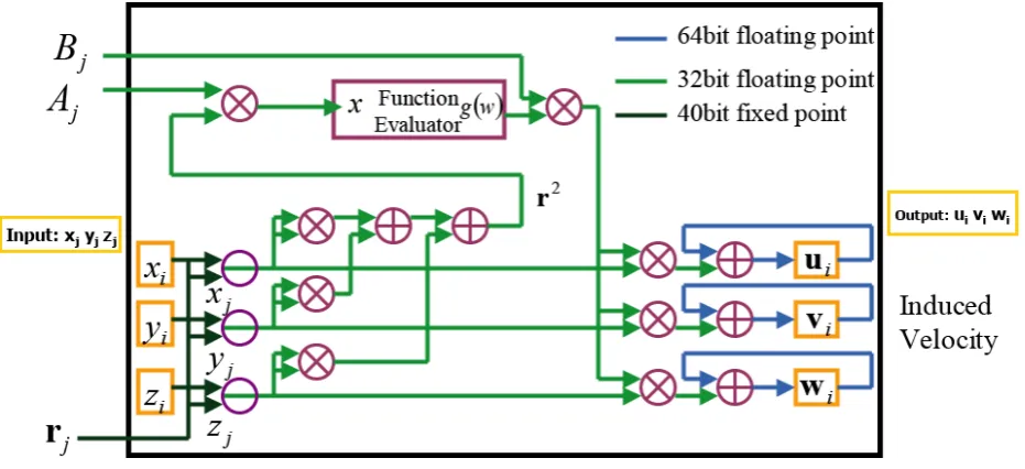
, respectively. These data are stored in registers and kept in the next six clock cycles. Peak performance of an MDGRAPE-2 chip corresponds to about 16 GFlops at a clock frequency of 100 MHz.

An MDGRAPE-2 pipeline calculates the pair wise force f_i,jas:

 

2 (7)

,j ij ij ij ij i b g a r r

f 

where g() is an arbitrary central force, and aij and bij are coefficients determined by particle types of particles i and j. The function g() for an arbitrary

value a|rij| 2

is calculated by interpolation, from values that are tabulated prior to the execution of the main program. If the interparticle distance is such that a|rij|

2

falls out of this tabulated domain, the MDGRAPE-2 assumes g() is zero. The number of tabulated points is constant. Thus, defining the table in a large domain would result in larger spacing between the tabulated points, and therefore a larger interpolation error. On the contrary, defining the table in a small domain would yield a higher probability that the inter particle spacing would fall outside the tabulated domain, which can also cause errors.

Figure 1 shows the block diagram of the pipeline of an MDGRAPE-2 chip. The pipeline calculates rij and

2

ij ijr

a , and then evaluate g() in the function evaluator. Function evaluator performs fourth-order interpolation segmented by 1,024 regions. The coefficients of the interpolation function are stored in the RAM in function evaluator. Therefore, it can be used any arbitrary central force by changing the contents of the RAM. After the function evaluator, the pipelines multiplies bij and rij, and then accumulates them. The relative accuracy of a pair wise force is about 10-7, since most of the arithmetic units in the pipeline use IEEE754 single floating point format.

173

The double floating point format is used for accumulating the force in order to prevent the underflow when large number of particles is used. 3.2 Calculation Procedures

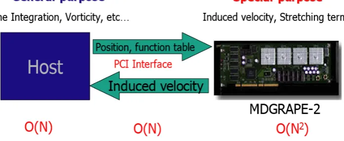
Figure 2 represent the system that performs vortex method calculations, consisting of a host and MDGRAPE-2. The host is a PC or a workstation. MDGRAPE-2 consists of one or multiple MDGRAPE-2 boards. Each board is connected to the host as an extension board via a PCI bus (or PCI buses linked by PCI-PCI bridges). A special-purpose computer work as a back-end hardware and the host PC work as a front-end processor. The host computer calculates and updates the positions of particles and sends it to special-purpose computer. The special-purpose computer then calculates the induced velocity by using Biot-Savart law and stretching term, which dominate the total calculation cost.

Since the load on MDGRAPE-2 is much heavier than those for host computer and communication interfaces between them, the total performance of the system is determined by the super-high-speed special-purpose computers rather than the host computer or communications, for a large number of particles. When the system performs VM simulations, MDGRAPE-2 calculates velocity from Biot-Savart law and Stretching term from vorticity equation. The host performs the other tasks such as giving the initial

state of particles, time integration and the control of MDGRAPE-2. The host sends necessary data for velocity or potential calculation to MDGRAPE-2 and receives velocity or potential from it via PCI bus (or the PCI buses).

A single board increases the computing speed of an ordinary PC to 64GFlops comparable to a supercomputer. The calculation of interactions between particles as represented by potential and force are carried out in MDGRAPE-2. In case of calculating the potential,

 









(8)

1

2 2

1





 

 

 N

j

ij ij ij ij N

j ij

i b g w b g a r



Φ

and the force calculations

 









(9)

1

2 2

1

ij N

j

ij ij ij ij ij

N

j ij

i b g wr b ga r r

f





 

 





are treated similarly, where g(w) is an arbitrary function equivalent to an intermolecular force, and aij, bij, and



_ijare arbitrary coefficients which are settled down for every model. To apply these libraries to the calculation of a vortex method, Biot-Savart law in Eq. (3) is expressed as follows.









(10)

1

2 2

ij N

j

ij ij j j

i B g A r r

u











where Aj, Bj are arbitrary constants and g() is an arbitrary function which has been explained

previous section 3.1. The details mathematical formulations are introduced in [15].

3.3 Performances

The peak performance of the MDGRAPE-2 board is 64GFlops at 250MHz PC when the board calculates Coulomb forces for 30000 or more particles. This performance is not the same when vortex method has been calculated using this board. The CPU-time is shown in Figure 3.

The computation time has been preformed and compared with ordinary PC (Intel Pentium 4 2.66GHz). The CPU-time has been calculated from Biot-Svart law (Eq. 3) and run for one time step while the number of particles is increased. Figure 3 shows the calculation time against the number of vortex elements N with and without the use of MDGRAPE-2. The CPU-time has been achieved for the calculation of flow around a circular cylinder. The legends 'Intel P4 (2.66GHz)' and 'MDGRAPE-2' represent the calculation time without and with the use of MDGRAPE-2, respectively. It is clearly observed that the calculation time is reduced by a factor of 100 for N~105. This acceleration rate is below the expected rate, but it can be improved by reducing the number of calls to the MDGRAPE-2 library for cross product calculations.

4. NUMERICAL RESULTS AND

DISCUSSION

We have applied our method to calculate the flow around a circular cylinder. The flow around a (geometrically) two-dimensional circular cylinder is case that has been used both as a validation case and as a legitimate research case. At very low Reynolds numbers, the flow is steady and symmetrical. As the Reynolds number is increased, asymmetries and time-dependence develop, eventually resulting the famous Von Karmann vortex street, and then on to turbulence. The problem geometry is two-dimensional and there is some variation in the details (both geometry and boundary conditions) that can be used. The exterior boundaries are generally placed very far from the cylinder surface to avoid interaction between the boundary conditions.

Figure 3. Performance of bluff body calculation

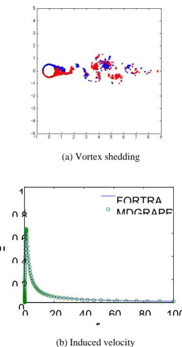
(a) Vortex shedding

0 20 40 60 80 100 0

0 2 0 4 0 6 0 8 1

r u

FORTRA MDGRAPE

(b) Induced velocity

175

We first calculate the convection of vortex elements using Adams-Bashforth time advancement. Then we calculate the induced velocity using Biot-Savart law (Eq. 3). Finally we investigate numerical error by calculating the difference between particles in different steps and drag and lift force coefficient to validate our proposed scheme.

Vortex elements were shed from each element on the wall. For this case, the vortex elements were shed only once and the convection of these elements were evaluated. The Karman vortex street has been observed from the vortex shedding shown in figure 4(a). Figure 4(b) represents the corresponding induced velocity of convection of vortex elements. It has been observed that the host PC gives better results until 512 vortex elements and beyond that it has coincided with MDGRAPE-2 calculation. It means that for accurate calculations large number of vortex elements is required.

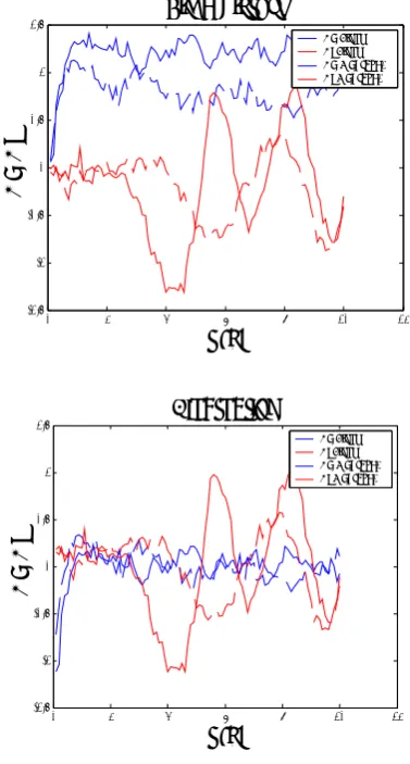
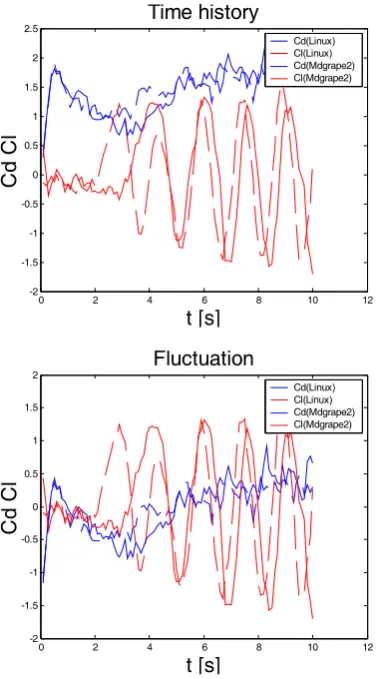
Cutoff function for host calculation and function evaluator for MDGRAPE-2 calculation has been considered. Both calculated results compared each other. The Figure 5 represent compared error and error difference between host and MDGRAPE-2 computer. It can be observed from the error calculations that host machine gives better results until 512 vortex elements and beyond that it has coincide with MDGRAPE-2 calculation. Drag (Cd) is a mechanical force generated by a solid object moving through a fluid. The lift coefficient (Cl) is a dimensionless coefficient that

relates the lift generated by a body, the dynamic pressure of the fluid flow around the body, and the platform area of the body. It may also be described as the ratio of lift pressure to dynamic pressure. Figures 6 and 7 represent the drag and lift coefficients for both calculations and compared the results. It is observed that for 50,000 elements they almost coincide for both calculations.

5. CONCLUSION

Special purpose computer MDGRAPE-2 for molecular dynamics was applied to calculation of vortex method, and improvement in the speed was attained. It has been calculated for up to 50,000 vortex elements and accelerated the calculation

10-40 10-20 100 1020

10-10

10-5

100

h

error

Host

MD-GRAPE2

Figure 5. Error between Host and MDGRAPE-2

0 2 4 6 8 10 12

-1.5 -1 -0.5 0 0.5 1 1.5

t [s]

Cd

Cl

Time history

Cd(Linux) Cl(Linux) Cd(Mdgrape2) Cl(Mdgrape2)

0 2 4 6 8 10 12

-1.5 -1 -0.5 0 0.5 1 1.5

t [s]

C

d Cl

Fluctuation

Cd(Linux) Cl(Linux) Cd(Mdgrape2) Cl(Mdgrape2)

using MDGRAPE-2 machine. Error has been compared and compared for drag and lift coefficients for every cases. Fluid-structure interaction must be considered in flows around flexible structures. It was observed that MDGRAPE-2 has reduced computation cost 100 times compared to Intel P4(2.66GHz) PC.

6. REFERENCES

1. Barba LA. Vortex Method for computing high-Reynolds number flows: Increased accuracy with a fully mesh-less formulation, PhD Thesis, California Institute of Technology, 2004.

2. Chatelain P. Contributions to the Three-Dimensional Vortex Element Method and Spinning Bluff Body Flows, PhD Thesis, California Insitute of Technology, 2005.

3. Cocle R, Winckelmans G, Daeninck G. Combining the vortex-in-cell and parallel fast multipole methods for efficient domain decomposition simulations, Journal of

Computational Physics, Vol. 227, No. 21, (2008),

9091-9120.

4. Cottet GH, Koumoutsakos PD. Vortex Methods (Theory and Practice), Cambridge University Press, 2000.

5. Eldredge JD. Dynamically coupled fluid-body interactions in vorticity-based numerical simulations,

Journal of Computational Physics, Vol. 227, No. 21,

(2008), 9170-9194.

6. Fukushige T, Taiji M, Makino J, Ebisuzaki T, Sugimoto D. A highly parallelized special-purpose computer for many-body simulations with an arbitrary central force: MD-GRAPE, Astrophys. J., (1996), 468:51.

7. Huang MJ, Su H-X , Chen L-C. A fast resurrected core-spreading vortex method with no-slip boundary conditions, Journal of Computational Physics, Vol. 228, No. 6, (2009), 1916-1931.

8. Leonard A. Vortex Methods for Flow Simulations. J

Comput Phys, Vol. 37, (1980), 289-335.

9. Liu CH, Doorly DJ. Vortex particle-in-cell method for three-dimensional viscous undbounded flow computations, Int. J. Numer. Meth. Fluids, Vol. 32, (2000), 29-50.

10. Narumi T. Special-Purpose Computer for Molecular Dynamics Simulations, Doctoral Thesis, College of Arts and Sciences, University of Tokyo, 1997.

11. Ploumhans P, Winckelmans GS, Salmon JK, Leonard A, and Warren MS. Vortex Methods for Direct Numerical Simulation of Three-Dimensional Bluff Body Flows: Application to the Sphere at Re = 300, 500, and 1000. J. Comp. Phys., Vol. 178, (2002), 427-463.

12. Poncet P. Analysis of an immersed boundary method for three-dimensional flows in vorticity formulation,

Journal of Computational Physics, Vol. 228, No. (19),

(2009), 7268-7288.

13. Ramachandran P, Ramakrishna M, Rajan SC. Efficient random walks in the presence of complex two- dimensional geometries, Computers & Mathematics

with Applications, Vol. 53, No. 2, (2007), 329-344.

14. Sbalzarini IF, Walther JH, Bergdorf M, Hieber SE, Kotsalis EM, Koumoutsakos P. PPM - A Highly Efficient Parallel Particle-Mesh Library for the Simulation of Continuum Systems. J. Comp. Phys. Vol. 215, (2006), 566-588.

15. Sheel TK, Yasuoka K, Obi S. Fast vortex method calculation using a special-purpose computer,

Computers and Fluids, Vol. 36, (2007), 1319-26.

16. Susukita R, Ebisuzaki T, Elmegreen B G, Furusawa H, Kato K, Kawai A, Kobayashi Y, Koishi T, McNiven GD, Narumi T, Yasuoka K. Hardware accelerator for molecular dynamics: MDGRAPE-2. Comput Phys

Comm, Vol. 155, (2003), 115-131.

17. Winckelmans GS, Leonard A. Contributions to Vortex Particle Methods for the Computation of Three- Dimensional Incompressible Unsteady Flows. J

Comput Phys, Vol. 109, (1993), 247-273.

18. Yatsuyanagi Y, Ebisuzaki T, Hatori T, Kato T. Filamentary magneto hydrodynamic simulation model, current vortex method. Physics of Plasmas, Vol. 10, (2003),3181-3187.

 

0 2 4 6 8 10 12

-2 -1.5 -1 -0.5 0 0.5 1 1.5 2 2.5

t [s]

Cd

Cl

Time history

Cd(Linux) Cl(Linux) Cd(Mdgrape2) Cl(Mdgrape2)

 

0 2 4 6 8 10 12

-2 -1.5 -1 -0.5 0 0.5 1 1.5 2

t [s]

Cd

Cl

Fluctuation

Cd(Linux) Cl(Linux) Cd(Mdgrape2) Cl(Mdgrape2)