HOMOTOPY PERTURBATION METHOD FOR SOLVING FLOW IN THE EXTRUSION PROCESSES

(1)

IJE Transactions A: Basics Vol. 23, Nos. 3 & 4, November 2010 - 267

HOMOTOPY PERTURBATION METHOD FOR SOLVING FLOW

IN THE EXTRUSION PROCESSES

M.M. Rashidi

Mechanical Engineering Department, Engineering Faculty of Buali Sina University, Hamedan, Iran [email protected]

D.D. Ganji

Mechanical Engineering Department, Engineering Faculty of Mazandaran University, Babol, P.O. Box 484, Iran [email protected]

(Received: August 26, 2009 – Accepted in Revised Form: November 2010) Abstract In this paper, the homotopy perturbation method (HPM) is considered for finding approximate solutions of two-dimensional viscous flow. This technique provides a sequence of functions which converges to the exact solution of the problem. The HPM does not need a small parameters in the equations, but; the perturbation method depends on small parameter assumption and the obtained results. In most cases, it ends up with a non-physical result, so homotopy perturbation method overcomes completely the above shortcomings. HPM is very convenient and effective and the solutions is compared with the exact solution.

Keywords: Homotopy Perturbation Method; Viscous; Extrusion Processes.

ﻩﺪﻴﻜﭼ

ﺍﺭﺩ ﻳ ﭘﻮﺗﻮﻤﻫﻝﻼﺘﺧﺍﺵﻭﺭﻪﻟﺎﻘﻣﻦ ﻲ

(HPM)

ﺍﺮﺑ ﻱ ﻳ ﺎﻫﻞﺣﻩﺍﺭﻦﺘﻓﺎ ﻱ

ﺮﻘﺗ ﻳﺒ ﻲ ﺮﺟ ﻳ ﻥﺎ ﺪﻌﺑﻭﺩﺝﺰﻟ ﻱ

ﺮﻈﻧﺭﺩ

ﺖﺳﺍﻩﺪﺷﻪﺘﻓﺮﮔ

.

ﺍﻳ ﻟﺍﻮﺗ،ﺵﻭﺭﻦ ﻲ

ﺎﻫﺩﺮﮑﻠﻤﻋ ﻲﻳ ﻣﻪﺋﺍﺭﺍﺍﺭ ﻲ ﻗﺩﻞﺣﻩﺍﺭﻪﺑﻪﮐﺪﻫﺩ ﻴ

ﻣﺍﺮﮕﻤﻫﻪﻠﺌﺴﻣﻖ ﻲ

ﺩﻮﺷ

.

ﺵﻭﺭ

ﭘﻮﺗﻮﻤﻫﻝﻼﺘﺧﺍ ﻲ

ﻧﻴ ﺎﻫﺮﺘﻣﺍﺭﺎﭘﻪﺑﺯﺎ ﻱ

ﺎﻫﺮﺘﻣﺍﺭﺎﭘﺽﺮﻓﻪﺑﻝﻼﺘﺧﺍﺵﻭﺭﺎﻣﺍ،ﺩﺭﺍﺪﻧﻪﻟﺩﺎﻌﻣﺭﺩﮏﭼﻮﮐ ﻱ

ﺎﺘﻧﻭﮏﭼﻮﮐ ﻳ

ﺞ

ﺖﺳﺍﻪﺘﺴﺑﺍﻭﻩﺪﻣﺁﺖﺳﺪﺑ

.

ﺁ،ﺩﺭﺍﻮﻣﺐﻠﻏﺍﺭﺩ ﺘﻧﻪﺑﻥ

ﻴ ﻏﻪﺠ ﻴ ﻓﺮ ﻴﺰ ﻳ ﮑ ﻲ ﻣﻢﺘﺧ ﻲ ﺩﻮﺷ

.

ﺍﺮﺑﺎﻨﺑ ﻳ ﭘﻮﺗﻮﻤﻫﻝﻼﺘﺧﺍﺵﻭﺭ،ﻦ ﻲ

ﺎﻫﺩﻮﺒﻤﮐﺮﺑﻼﻣﺎﮐ ﻱ

ﻣﻪﺒﻠﻏﻻﺎﺑ ﻲ ﺪﻨﮐ

.

ﭘﻮﺗﻮﻤﻫﻝﻼﺘﺧﺍ ﻲ

ﺴﺑﺵﻭﺭ ﻴ

ﻞـﺣﻩﺍﺭﺎـﺑﺎﻫﻞﺣﻩﺍﺭﻭﺖﺳﺍﺮﺛﻮﻣﻭﺐﺳﺎﻨﻣﺭﺎ

ﻗﺩ ﻴ ﺎﻘﻣﻖ ﻳ ﻣﻪﺴ ﻲ ﺩﻮﺷ

.

1. INTRODUCTION

Most of engineering problems, especially heat transfer and fluid flow equations are nonlinear. Therefore, some of them are solved using computational fluid dynamic (numerical) method and the other using analytical perurbation method [1-3]. In the numerical method, stability and convergence should be considered to avoid divergent or inappropriate results. In analytical perturbation method, the small parameter should be exerted in the equation [4]. Thus, finding the small parameter and exerting it into the equation are the problems of this method. The perturbation method is one of the well-known methods to solve the nonlinear equations which was studied by a large number of researchers such as Bellman [5] and Cole [6]. Actually, these scientists paid more attention to the mathematical aspects of the subject which included a loss of physical verification. This loss in the physical verification of the subject was recovered by Nayfeh [7] and Van Dyke [8].

In recent years, an increasing interest of scientist and engineers in analytical techniques for studying nonlinear problems was appeared. Such techniques have been dominated by the perturbation methods and have found many applications in science, engineering and technology. However, like other analytical techniques, the perturbation methods have their own limitations. For example, all the perturbation methods require the presence of a small parameter in the nonlinear equation and approximate solutions of equation containing this parameter are expressed as series expansions in small parameter. Selection of small parameter requires a special skill. A proper choices of small parameter gives acceptable results, while an improper choice may result in incorrect solutions. Therefore, an analytical method is welcome which does not require a small parameter in the equation modeling the phenomena.

(2)

268- IJE Transactions A: Basics Vol. 23, Nos. 3 & 4, November 2010 common perturbation method was upon the existence

of a small parameter, developing the method for different applications is very difficult. Therefore, many different new methods have recently introduced some ways to eliminate the small parameter such as artificial parameter method by Liu [9], the homotopy analysis method (HAM) by Liao [10] and the variational iteration method (VIM) by He [11-12, 21-22]. One of the semi-exact methods is HPM [13-16] and other methods are also introduced [23]. In this paper, we solve the flow field due to stretching boundary with partial slip by HPM. The flow due to a stretching boundary is important in extrusion processes. The bathing fluid is entrained by the tangential velocity of the extrusate and thus affects convective cooling [17]. Vleggaar experimentally showed the velocity of an extrusate which is initially proportional to the distance from the orifice [18]. The boundary condition are similar to those due to a stretching surface and exact solutions of the Navier-Stokes equations can be found [19].

2. BASIC CONCEPTS OF HPM

We consider the following ODE

( )

0,

,

A u

−

f r

=

r

∈Ω

₍₁₎ (1)

subject to boundary condition

( ,

u

)

0,

.

B u

r

n

∂ =

∈Γ

∂

(2)

The operator

A

can, generally speaking, be divided into two parts: a linear part

L

and a nonlinear part

N

.

Therefore, equation (1) can be rewritten as follows:

( )

0,

L v

+

N v

−

f r

=

₍₃₎ (3)

we construct a homotopy of equation (1)

( , ) :

[0,1]

v r p

Ω×

→ ℜ

which satisfies

0

( , )

(1

) [ ( )

(

)]

[ ( )

( )],

[0,1, ],

,

H v p

p

L v

L u

p A v

f r

p

r

= −

−

+

−

∈

∈ Ω

(4)

where

p

∈

[0,1]

is an embedding parameter and

u

₀ is an initial guess approximation of equation (3) which satisfies the boundary conditions.

3. GOVERNING EQUATIONS

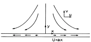
Consider a two-dimensional stretching boundary (Fig. 1) where the lateral surface velocity is proportional

Figure 1. Two dimensional viscous flow

to the distance

x

from the origin. The velocity is as follows:

.

U

=

a x

(5) Let

( , )

u v

be the fluid velocities in

x

and

y

directions, respectively. The Navier’s condition is then [17]

( , 0)

u

( , 0),

u x

U

k

x

y

υ

∂

− =

∂

(6)

where

k

is a proportional constant and

υ

is kinematic viscosity of the bulk fluid. The steady 2-D Navier-Stokes equations can be written as

0,

x y

u

+ =

v

(7)

(

)

/ ,

x y xx yy x

u u

+

v u

=

υ

u

+

u

−

p

ρ

(8)

(

)

/ ,

x y xx yy y

u v

+

v v

=

υ

v

+

v

−

p

ρ

(9) where

p

and

ρ

are pressure and density, respectively. For solving equations (7)-(9), we must apply boundary conditions (equations (5) and (6)). Other boundary conditions are no lateral velocity and pressure gradient far from the stretching surface. For similarity solutions we set [17]:

( ),

u

=

a x f t

′

(10)

( ),

v

= −

a

υ

f t

(11)

/ .

t

=

y a

υ

(12) Continuity equation automatically is satisfied. equation (8) can be written as follows:

2

( )

0,

f

′′′

t

−

f

′

t

+

f t f t

′′

=

₍₁₃₎

with the boundary conditions

(0)

0,

f

=

(14)

( )

0,

f

′ ∞ =

(15)

(0)

(0) 1.

f

′

=

K f

′′

+

(3)

IJE Transactions A: Basics Vol. 23, Nos. 3 & 4, November 2010 - 269 equation (6) and

K

=

k

aυ

is a non-dimensional

parameter indicating the relative importance of partial slip. For

K

=

0

, the fluid is inviscid.

In this section, HPM is used to find approximate solutions of the equation (13). Suppose the solution have the form as below:

2

0 1 2

3 4 5

( )

,

f t

p f t

=

+

L

(17)

if we apply Eq. (4) to Eq. (13), then

2

(1

)

( )

0

p f

t

p f

t

f

t

f t f

t

′′′

−

+

′′′

′

′′



−

+

=



=





(18) (18)

Then substituting equation (17) into equation (18) and rearanging based on powers of

p

- terms, we have

0 0

:

0,

p

f

′′′ =

(19) (19)

1 2

1 0 0 0

:

0,

p

f

′′′

−

f

′

+

f f

′′

=

(20) (20)

2

2 0 1 0 1 1 0

:

2

0,

p

f

′′′

−

f f

′ ′

+

f f

′′

+

f f

′′

=

(21) (21)

3 2

3 1 0 2 0 2

1 1 2 0

:

2

0,

p

f

f f

′′′

−

′

−

′ ′

+

′′

+

′′

+

′′

=

(22) (22)

4

4 0 3 1 2 0 3

1 2 2 1 3 0

:

2

0,

p

f

f f

′′′

−

′ ′

−

′ ′

+

′′

+

=

(23) (23)

5 2

5 2 0 4 1 3 0 4

1 3 2 2 3 1 4 0

:

2

0,

p

f

f f

′′′

−

′

−

′ ′

−

′ ′

+

′′

+

=

(24) (24)

6

6 0 5 1 4 2 3 0 5

1 4 2 3 3 2 4 1 5 0

:

2

0,

p

f

f f

′′′

−

′ ′

−

′ ′

−

′ ′

+

′′

+

′′

+

′′

+

′′

+

′′

+

′′

=

(25) (25)

7 2

7 3 0 6 1 5

2 4 0 6 1 5 2 4

3 3 4 2 5 1 6 0

:

2

0,

.

p

f

f f

′′′

−

′

−

′ ′

−

′ ′

−

′′

′ ′ +

+

′′

+

′′

+

′′

+

′′

=

L

(26)

To determine

f t

( )

, the above equations should be solved with appropriate boundary conditions (equations (14)-(16)). The solutions of above equations for

0

K

=

and

K

=

20

, are as follows

15 16 17 18 31 116383 ( ) 1307674368000 20922789888000 626881 419 355687428096000 12934088294400

f t t t

t t = − − + − (27) 19 20 1718011 70525699

11058645491712000t 2432902008176640000t

+ +

21 22

1323139 6597271

4644631106519040000t 28820531481477120000t

− −

23 2

3 4 5 6 7

18992159 1

1988616672221921280000 2

1 1 1 1 1

6 24 120 720 5040

t t t

t t t t t

+ + −

+ − + − + +

8 9 10 11

12 13

1 1 13 13

13440 51840 1209600 4435200

29 307

479001600 1245404160

t t t t

t t − − + + − 14 839 12454041600t + (27) and 18 19 26454129170347965799 ( ) 1335965400000000000000000000000000000000 34981592008374802708157 290095344000000000000000000000000000000000

f t t

t = − − + 20 2 9610620390380100302367991 1099944846000000000000000000000000000000000000 0.124 0.0219 t t t + − 15

3 5 4

152109012706142059

1135134000000000000000000000000000

961 15987 2263

375000 1000000000 10000000

t

t t t

− + + − 21 6636411496225660841695231 146659312800000000000000000000000000000000000000t − 16 94928946234172707119 1089728640000000000000000000000000000t − 22 4137391052244534387257825723 483975732240000000000000000000000000000000000000000t − + 7 6 7342381 70153

157500000000000t −75000000000t +

23

1384631564415805048337910253

10703309463000000000000000000000000000000000000000000t +

8 10

49660951 679770225707

14000000000000000t −7560000000000000000000t −

9 11

3799829309 30866371688293

5670000000000000000t +3118500000000000000000000t +

17

470250127393223949061

42882840000000000000000000000000000000t −

(4)

270- IJE Transactions A: Basics Vol. 23, Nos. 3 & 4, November 2010

14

28171951570650389

.

2837835000000000000000000000000t ₍₂₈₎

(28) When

K

=

0

, Crane [20] found the exact solution

( ) 1 t. f t = −e−

(29) (29) The perturbation solution for small

K

is

( ) 1 (1 ) 1

2

t K t

f t = −e− + _ −t e− − +_

(30)

{

}

2

3

0.087459 1.221835(1 ) 0.25 ( ) 5

( ),

t t t

K e t e h e t

O K

− ₊ ₊ − ₋ _ − _{− +} _

 

+

(30)

2 3 4

5 6

1 1 1

( )

4 72 864

1 1

.

9600 108000

h t t t t

t t

= − +

− + −L (31)

(31)

4. DISCUSSION

In this paper, the HPM is used to find approximate solutions of two-dimensional Navier-Stokes equations. In this work, we use the Maple Package to solve the obtained differential equations. In Table 1, we compare obtained values for

f

( )

∞

by the HPM and the numerical method.

TABLE 1. Comparison between

f

( )

∞

by HPM and numerical method.

K 0.3 1 2 5 20

HPM method

0.84021 0.70068 0.601230.46442 0.31119

Numerical method

[17]

0.887 0.748 0.652 0.514 0.322

The accuracy of the method is very good and obtained results are near to the exact solution. The approximate solution obtained in Fig. 2 in comparison with exact solution admit a remarkable accuracy.

t

f(

t)

0 1 2 3

0 0 . 2 0 . 4 0 . 6 0 . 8 1

E x a c t H P M ( K = 0 )

Figure 2. Comparison of the exact and approximate solution obtained by HPM

t

f(

t)

0 1 2 3

0 0 . 2 0 . 4 0 . 6 0 . 8 1

H P M ( K = 0 . 3 ) P e r t u r b a t i o n ( K = 0 . 3 )

Figure 3. Comparison of the approximate solution obtained by HPM and the perturbation method.

t

f(

t)

0 1 2 3

0 0.2 0.4 0.6 0.8 1 1.2 1.4

HPM (K=1) Perturbation (K=1)

(5)

IJE Transactions A: Basics Vol. 23, Nos. 3 & 4, November 2010 - 271 t

f(

t)

0 1 2 3

0 0.5 1 1.5 2 2.5 3 3.5

HPM (K=2) Perturbation (K=2)

Figure 5. Comparison of the approximate solution obtained by HPM and the perturbation method

The approximate solutions of function

f t

( )

have been shown in the Figs. 3-5. The approximate solutions by the perturbation method is only valid for small values of K . For example the approximate solutions that are presented in Figs. 4 and 5 are nonphysical solutions, because the value of

f t

( )

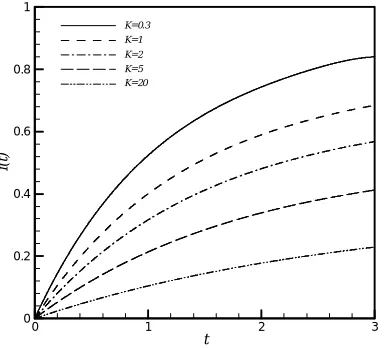
must be less (or equal ) than one for different values of K parameter. In the Figs. 6 and 7, the approximate solutions of f t( ) and

( )

f ′t for different values of K are presented. Figs. 8 and 9 show the velocities in

x

and

y

directions, respectively.

t

f(

t)

0 1 2 3

0 0.2 0.4 0.6 0.8 1

K=20 K=5 K=2 K=1 K=0.3

Figure 6. The approximate solutions of f t( ) for different values of K

t

f

'(

t)

0 1 2

0 0.2 0.4 0.6 0.8 1

K=20 K=5 K=2 K=1 K=0.3

Figure 7. The approximate solutions of f ′( )t for different values of K

Figure 8. The distribution of velocity in x direction versus , .x t

t

v(

t)

0 1 2 3

0 0.0002 0.0004 0.0006 0.0008 0.001 0.0012

K=20 K=5 K=2 K=1 K=0.3

(6)

272- IJE Transactions A: Basics Vol. 23, Nos. 3 & 4, November 2010

5. REFERENCES

[1] A. Rajabi, D. D. Ganji, H. Taherian, Application of homotopy perturbation method in nonlinear heat conduction and convection equations, Physics Letters A, Vol. 360 (2007) 570-573.

[2] D. D. Ganji, A. Rajabi, Assessment of homotopy– perturbation and perturbation methods in heat radiation equations, International Communications in Heat and Mass Transfer, Vol. 33 (3), (2006) 391- 400.

[3] A. M. Siddiqui, M. Ahmed, Q. K. Ghori, Thin film flow of non-Newtonian fluids on a moving belt, Chaos, Solitions and Fractals, Vol. 33, (2007), 1006-1016. [4] D. D. Ganji, The application of He’s homotopy

perturbation method to nonlinear equations arising in heat transfer, Physics Letters A, Vol. 355, (2006), 337-341. [5] R. Bellman, Perturbation techniques in mathematics,

Physics and Engineering, Holt, Rinehart & Winston, New York, 1964.

[6] J.D. Cole, Perturbation methods in applied mathematics, Blaisedell, Waltham, MA, 1968.

[7] A. H. Nayfeh, Perturbation methods, Wiley, NewYork , 1973.

[8] M. VanDyke, Perturbation methods in fluid mechanics, Annotated edition, Parabolic press, Stanford, CA, 1975. [9] G.L. Liu, New research directions in singular perturbation

theory artificial parameter approach and inverse-perturbation technique, Conference proceedings of 7th modern mathematics and mechanics, Shanghai, 1997. [10] S.J. Liao, An approximate solution technique not

depending on small parameters: a special example, Int. J. Non-Linear Mech, Vol. 303, (1995), 371-380.

[11] J.H. He, Approximate analytical solution for seepage flow with fractional derivatives in porous media, J. Comput. Math. Appl. Mech. Eng., Vol. 167, (1998), 57-68.

[12] J.H. He, Variational iteration method: a kind of nonlinear analytical technique: some examples, Int. J. Non-Linear Mech. Vol. 344, (1999), 699- 703.

[13] J. H. He, Newton-like method for solving alegbraic

equations. Commun Nonlinear Sci Numer Simulat, Vol. 3(2) (1998), 106-109.

[14] J. H. He, Comparison of homotopy perturbation and homotopy analysis method. Appl. Math. Comput., Vol. 156, (2004), 359-527.

[15] J. H. He, Homotopy perturbation method: a new nonlinear analytical technique. Appl. Math. Comput., Vol. 135, (2003), 73-79.

[16] J. H. He, Asymptotology by homotopy perturbation method. Appl. Math. Comput., Vol. 156, (2004), 591-596.

[17] C. Y. Wang, Flow due to a stretching boundary with partial slip-an exact solution of the Navier-Stokes equations. Chemical Engineering Science, Vol. 57 (2002), 3745-3747.

[18] J. Vleggaar, Laminar boundary-layer behavior on continuous accelerated surfaces. Chemical Engineering Science, Vol. 32, (1977), 1517-1525.

[19] C. Y. Wang, The three dimensional flow due to a stretching flat surface. Physics of Fluids, Vol. 27, (2002), 1915-1917.

[20] S. R. Seyed Alizadeh. G, G. Domairry, S. Karimpour, An approximation of the analytical solution of the linear and nonlinear integro-differential equations by homotopy perturbation method, Acta Applicandae Mathematicae. doi: 10.1007/s10440-008-9261-z.

[21] Hafez Tari, D.D. Ganji , H. Babazadeh, The application of He’s variational iteration method to nonlinear equations arising in heat transfer, Physics Letters A; Vol. 363, (2007), 213–217.

[22] D. D. Ganji , H. Babazadeh, M. H. Jalaei, H. Tashakkorian, Application of He’s Variational Iteration Methods for solving nonlinear BBMB equations and free vibrations of systems, Acta Applicandae Mathematicae, doi: 10.1007/s10440-008-9303-6.

[23] S. H. Hosein-Nia, A. Ranjbar N., H. Soltani, J. Ghasemi, Effect off the initial approximation on stability and convergence in homotopy perturbation method,