Scalable Computing: Practice and Experience
Volume 19, Number 3, pp. 275–291. http://www.scpe.org
ISSN 1895-1767 c
⃝2018 SCPE
ANALYSIS OF MEMORY FOOTPRINTS OF SPARSE MATRICES PARTITIONED INTO UNIFORMLY-SIZED BLOCKS∗
D. LANGR† ‡AND I. ˇSIME ˇCEK†
Abstract. The presented study analyses memory footprints of 563 representative benchmark sparse matrices with respect to their partitioning into uniformly-sized blocks. Different block sizes and different ways of storing blocks in memory are considered and statistically evaluated. Memory footprints of partitioned matrices are then compared with their lower bounds and CSR, index-compressed CSR, and EBF storage formats. The results show that block-based storage formats may significantly reduce memory footprints of sparse matrices arising from a wide range of application domains. Additionally, measured consistency of results is presented and discussed, benefits of individual formats for storing blocks are evaluated, and an analysis of best-case and worst-case matrices is provided for in-depth understanding of causes of memory savings of block-based formats.
Key words: block, memory footprint, partitioning, sparse matrix, storage format
AMS subject classification. 65F50
1. Introduction. The way how sparse matrices are stored in a computer memory may have a significant impact on the required memory space, i.e., on the matrix memory footprints. Reduction of matrix memory footprints may positively influence related computations and executions of corresponding programs [14, 23, 20, 21]. One way of reducing memory footprints of sparse matrices is their partitioning into blocks. Much has been written about block processing of sparse matrices, frequently in the context of memory-bounded character of
sparse matrix-vector multiplication (SpMV) [3, 4, 5, 6, 7, 8, 9, 10, 13, 16, 17, 18, 19, 24, 25, 27, 28, 30, 29, 31, 32, 33, 34, 35]. In this article, we address the problem of minimizing memory footprints of sparse matrices by their partitioning into uniformly-sized blocks. Its solution raises two essential questions:
1. How to choose a suitable block size?
2. How to store resulting nonzero blocks in a computer memory?
These questions form a multi-dimensional optimization problem that needs to be solved prior to the partitioning itself. We refer to both these problems—optimization and partitioning—as (block)preprocessing.
The above introduced optimization problem raises another question: How to specify the optimization space, i.e., the space of tested configurations? Intuitively, the larger the optimization space is, the lower matrix memory footprint can be found, however, at a price of longer preprocessing runtime. To amortize block processing of a sparse matrix, the optimization space thus need to be chosen wisely in a form of a trade-off: we want it to be small enough to ensure its fast exploration but also large enough to contain the optimal or nearly-optimal configuration generally for any sparse matrix.
We present a study that analyses memory footprints of 563 representative sparse matrices from the Uni-versity of Florida Sparse Matrix Collection (UFSMC) [11] with respect to their partitioning into uniformly sized blocks. These matrices arose from a large variety of applications of multiple problem types and thus have highly diverse structural and numerical properties. Our goal is to minimize memory footprints of matrices and we consider an optimization space that consists of different block sizes and different ways of storing blocks in memory. Based on the obtained results, we finally provide suggestions for both efficient and effective block preprocessing of sparse matrices in general.
This article is an extended version of our conference paper [21]. It recapitulates main contributions of the paper and adds new material, which mainly covers following subjects:
1. To assess representativeness of benchmark matrices, we measured the consistency of results across randomly selected subsets of these matrices (see Section 3.5).
∗This work was supported by the Czech Science Foundation under grant no. 16-16772S and by the Czech Ministry of Education, Youth and Sports under Grant No. CZ.02.1.01/0.0/0.0/16 019/0000765.
†Department of Computer Systems, Faculty of Information Technology, Czech Technical University in Prague, Th´akurova 9, 160 00, Praha, Czech Republic ([email protected]).
‡V´yzkumn´y a zkuˇsebn´ı leteck´y ´ustav, a.s., Beranov´ych 130, 199 05, Praha, Czech Republic.
2. We investigated influence of individual storage formats to the results and show that there is practically no reason to use the CSR storage format for storing blocks (see Section 3.6).
3. Originally, memory footprints of matrices were compared with their lower bounds and with 32-bit indexed CSR storage format (CSR32), which is the most commonly used format in practice. However, in our block-based approach, we assume index compression. It makes therefore sense to compare memory footprints of matrices also with index-compressed implementation of CSR (see Section 3.8). 4. We show that the lower bound for matrix memory footprint is the amount of memory required to store
the values of matrix nonzero elements [25, 21]. However, in practice, we can approach this lower bound only if we make some assumptions about a matrix structure. Without such assumptions, i.e., in generic cases, we can define another lower bound for memory footprints of sparse matrices that stems from compression of data about matrix nonzero structure. This concept is used by so-called entropy-based format (EBF) and within this article, we present memory footprints of matrices compared to EBF as well (see Section 3.9).
5. We provide statistical analysis of measured memory footprints with respect to CSR32 as a function of some of their characteristics, namely their application domain, density of nonzero elements, and deviation of number of nonzero elements per rows (see Section 3.7).
6. We provide in-depth analysis of best-case and worse-case matrices, which are matrices most suitable and unsuitable for block processing, respectively. This analysis allows better understanding of our block-based concepts and may clarify some of their aspects (see Section 3.11).
Some parts of the original paper were shortened or omitted.
2. Methodology. In Section 1, we referred to a matrix memory footprint as to an amount of memory space required to store a given matrix in a computer memory. More precisely, we can define it as a number of bits (or bytes) that is needed to store the values of the nonzero elements of a given matrix together with the information about their structure, i.e., their row and column positions. The ways how sparse matrices are stored in a computer memory are generally calledsparse matrix storage formats; we call themformats only if the context is clear. Matrix memory footprint is thus a function of a given matrix and a used format (memory footprints for the same matrix but distinct formats may differ considerably).
2.1. Block Storage Schemes. In case of partitioned sparse matrices, their nonzero blocks represent individual submatrices that can be treated separately. In practice, well-proven formats used for nonzero blocks of sparse matrices are:
• The coordinate (COO) format, which stores values of block nonzero elements together with their row and column indices [6, 24, 30].
• Thecompressed sparse row (CSR) format, which stores values and column indices of lexicographically ordered block nonzero elements together with the information about which values / column indices belongs to which block row [24, 27, 28, 30].
• Thebitmapformat, which stores values of block nonzero elements in some prescribed order and encodes their row and column indices in a bit array [7, 18, 24].
• Thedense format, which stores values of both nonzero and zero block elements in a dense array (row and column indices of nonzero elements are thus effectively determined by positions of their values within this array) [2, 16, 17, 24].
Considering these formats, we have 6 options how to store nonzero blocks of a sparse matrix in memory: 1. store all the blocks in the COO format,
2. store all the blocks in the CSR format, 3. store all the blocks in the bitmap format, 4. store all the blocks in the dense format,
5. storeall the blocksin the same format such that the format minimizes the memory footprint of a given matrix (we refer to this option as min-fixed),
6. storeeach block generally in a different format such that the format minimizes the contribution of this block to the memory footprint of a given matrix (we refer to this option asadaptive).
For the min-fixed and adaptive schemes, we consider formats for nonzero blocks to be chosen from COO, CSR, bitmap, and dense. In case of the min-fixed scheme, the matrix memory footprint thus contains 2 additional bits for storing the information about the format used for all the nonzero blocks. In case of the adaptive scheme, the matrix memory footprint contains 2 additional bits for each nonzero block to store the information about its format.
2.2. Block Sizes. To evaluate memory footprints of a given matrix for different schemes and some par-ticular tested block size, we need information about numbers of nonzero elements of all nonzero blocks [24]. In the end, this information must be obtained for each distinct block size from the optimization space, which represents the most demanding part of the whole optimization process [22]. The block preprocessing runtime is thus approximately proportional to the number of distinct tested block sizes. Consequently, the lower is their count, the higher are the chances that the partitioning will be profitable at all.
Generally, there isO(m×n) ways how to set a block size for anm×nmatrix, but for fast block preprocessing, we need to choose only few of them.1 One possible approach is to consider only block sizes
2k×2ℓ, where 1≤k≤K and 1≤ℓ≤L, (2.1)
which reduces the number of tested block sizes to K×L. The rationale behind such a choice consists, e.g., of much faster block preprocessing, full employment of bits for storing in-block row and column indices, higher utilization of caches, and possible storage of block elements inZ-Morton order [26] (for detailed explanation of these aspects, see [21]).
Within the presented study, we consider block sizes (2.1) and set K =L= 8. The choice of these upper bounds stemmed from our auxiliary experiments which showed that space-optimal block sizes have mostly less than 64 rows/columns. Taking into account block sizes with up to 256 rows/columns should cover even the remaining corner cases.
Consequently, each m×n matrix is further treated as a set of block matrices of sizes ⌈m/2k⌉ × ⌈n/2ℓ⌉, where 1≤k, ℓ≤8.
2.3. Optimization Space. In the summary, our optimization space is initially defined byS6× B64, where S6 denotes a set of selected block storage schemes:
S6={COO,CSR,bitmap,dense,min-fixed,adaptive} (2.2)
andB64 denotes a set of selected block sizes:
B64={2k×2ℓ: 1≤k, ℓ≤8}. (2.3)
2.4. Additional Considerations. Additionally, when measuring matrix memory footprints, we need to decide how to represent information about nonzero blocks and how to represent indices. In the presented study, we assume:
1. nonzero blocks stored in memory in the lexicographical order; 2. explicit storage of block column index for each nonzero block; 3. storage of the number of nonzero blocks for each block row;
4. a minimum possible number of bits, i.e.,⌈log2n⌉bits, to store an index related to nentities (such an approach is in the literature sometimes referred to asindex compression).
2.5. Benchmark Matrices. Sparse matrices are often divided into two main categories—high perfor-mance computing (HPC) matrices andgraph matrices, the latter being binary matrices for unweighted graphs. Efficient processing of graph matrices is generally governed by special rules that are different from those being effective for HPC matrices [1, 8, 36] (e.g., higher matrix memory footprints in some cases lead to higher perfor-mance of computations and graph matrices are also typically not suitable for simple block processing mainly due
1In addition to multiplication and Cartesian product, we also use the multiplication sign “×” to specify matrix/block sizes. In
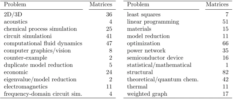
Table 2.1
Counts of tested matrices falling under particular problem types (referred to as “kinds” in the UFSMC).
Problem Matrices
2D/3D 36
acoustics 4
chemical process simulation 25
circuit simulationi 41
computational fluid dynamics 47
computer graphics/vision 8
counter-example 2
duplicate model reduction 5
economic 24
eigenvalue/model reduction 2
electromagnetics 11
frequency-domain circuit sim. 4
Problem Matrices
least squares 7
linear programming 51
materials 15
model reduction 11
optimization 66
power network 35
semiconductor device 16
statistical/mathematical 1
structural 82
theoretical/quantum chem. 42
thermal 11
weighted graph 17
to emergence of hypersparse blocks [7, 8]). Within this work, we focused mainly (but not exclusively) on HPC matrices. Particularly, for experiments, we took real matrices from the UFSMC that contained more than 105 nonzero elements and that exhibited a unique structure of nonzero elements.2 This way, we obtained 563 sparse matrices arising from different application problems (see Table 2.1) and thus having different structural (and numerical) properties; we denote these matrices byA1, . . . , A563. Of these matrices, 281 were square symmetric and the remaining 282 were either rectangular or square unsymmetric.
For symmetric matrices, we always assume storage only of their single triangular parts in memory, which is a common practice. When referring to the number of nonzero elements of a matrix, we thus generally need to distinguish between the number ofall nonzero elements and the number of elements that are assumed to be
stored in a computer memory. While measuring memory footprints of sparse matrices, we take into account the latter one.
2.6. Matrix Memory Footprint. According to the text above, a matrix memory footprint for a sparse matrixAk partitioned into uniformly-sized blocks is a function of the following parameters:
1. a sparse matrix itself (Ak), 2. a block storage schemes∈ S6, 3. a block size h×w∈ B64,
4. a number of bitsb required to store a value of a single matrix nonzero element.
We denote this function by MMF⊞(Ak, s, w×h, b). We further assume storing values of matrix nonzero elements in either single or double precision IEEE floating-point format [15], which impliesb= 32 orb= 64, respectively, in case of real matrices. We refer to such a floating-point precision as precision only.
We say that a matrix memory footprint for a given matrix A and a given precision determined by b is
optimal (with respect to our work) if it equals
min{
MMF⊞(A, s, h×w, b) :s∈ S6, h×w∈ B64}. (2.4)
We call the corresponding block storage scheme and block size optimal as well.
2.7. Optimization Subspaces. LetS ⊆ S6andB ⊆ B64. S ×Bthus define a subspace of the optimization spaceS6× B64. Let
∆bS,B(k) = (
min{
MMF⊞(Ak, s, h×w, b) :s∈ S, h×w∈ B }
min{
MMF⊞(Ak, s, h×w, b) :s∈ S6, h×w∈ B64} −1
)
×100. (2.5)
Table 3.1
Minimum, average and maximum values ofUb
s,B64 (in percents).
Single precision (b= 32) Double precision (b= 64)
Scheme (s) Minimum Average Maximum Minimum Average Maximum
COO 0.00 4.78 15.27 0.00 2.52 7.67
CSR 0.73 6.84 19.13 0.41 3.74 11.05
bitmap 0.00 3.13 22.01 0.00 1.75 12.38
dense 0.00 84.61 217.04 0.00 92.40 249.02
min-fixed 0.00 1.19 5.41 0.00 0.64 2.94
adaptive 0.00 0.10 2.24 0.00 0.05 1.30
This function expresses of how much percent is the minimal memory footprint ofAk fromS × Bhigher (worse) than its optimal memory footprint. To assess the subspaceS × B, we define the following parametrized set
Ub S,B=
{ ∆b
S,B(k) : 1≤k≤563 }
. (2.6)
The minimum, mean (average; µ), and maximum of Ub
S,B then reflect the best, average, and worst cases,
respectively, forS × Bacross the tested matrices. IfS orBconsists of a single element only, we omit the curly braces in the subscript ofU for the sake of readability; e.g., we writeUb
s,B64 andU
b
S6,h×w instead ofU b
{s},B64 and Ub
S6,{h×w}.
3. Results and Discussion.
3.1. Block Storage Schemes. First, we assessed block storage schemes. Complete statistics of Ub
s,B64
are presented in Table 3.1 and lead to the following observations:
• No fixed-format scheme minimized matrix memory footprints in comparison with the others. Bitmap was the best in average, however, it was inferior to both COO and CSR in worst cases.
• Dense provided extremely high matrix memory footprints in average and worst cases. Due to the explicit storage of zero elements, this scheme is suitable only for kinds of matrices that contain highly dense blocks; obviously, there were only few such matrices in our tested suite.
• The lowest memory footprints were provided by the min-fixed and adaptive schemes; their numbers are considerably lower in comparison with the fixed-format schemes.
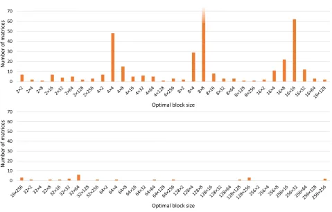
3.2. Block Sizes. Similarly as block storage schemes, we assessed block sizes. Figure 3.1 shows for how many tested matrices were individual block sizes optimal in case of double precision measurements; for single precision, the results differed only for 2 matrices. We may observe that some block sizes were especially favourable. The 8×8 block size was optimal for 257 matrices, which corresponds to 45.6% of their total count. Together with 4×4 and 16×16, these 3 block sizes were optimal for 65.2% of tested matrices. However, the numbers from Figure 3.1 reflect only best cases. To find out how much were particular block sizes better than the others in average and for their worst-cases matrices, we present the average and maximum values of Ub
S6,h×w in Tables 3.2 and 3.3 for single and double precision, respectively. According to these results, some blocks sizes—especially 8×8—provided alone average matrix memory footprints close to their optimal values. However, there was not a single block size that would yield the same outcome for all the tested matrices; the maxima were for all the block sizes relatively high.
3.3. Subsets of Block Sizes. Let us remind that one of our goals is a possible reduction of the number of block sizes in the optimization test space. The question thus is whether there is some subsetB ⊂ B64 that would, at the same time:
1. significantly reduce the number of block sizes (|B|),
2. provide matrix memory footprints close to their optimal values for most of the tested matrices (average ofUb
S6,B close to zero),
0 10 20 30 40 50 60 70
N
u
m
b
e
r
o
f
m
a
tr
ic
e
s
Optimal block size
0 10 20 30 40 50 60 70
N
u
m
b
e
r
o
f
m
a
tr
ic
e
s
Optimal block size
Fig. 3.1. Numbers of tested matrices for which are block sizes optimal, measured for double precision; block size8×8 was optimal for 257 matrices.
Table 3.2 Average and maximum values ofU32
S6,h×w (in percents), sorted by average.
.
Rank h×w Avg. Max.
1 8×8 1.23 18.36
2 8×16 2.14 19.35
3 16×8 2.26 21.41
4 4×8 2.32 17.31
5 8×4 2.38 19.52
6 16×16 2.56 21.82
7 4×4 2.92 21.94
8 4×16 2.99 16.51
9 16×4 3.23 20.44
10 8×32 3.65 21.26
Rank h×w Avg. Max.
11 16×32 4.03 23.75
12 32×8 4.13 23.97
13 4×32 4.36 18.71
14 32×16 4.53 24.45
15 32×4 4.87 23.60
16 32×32 5.20 26.50
. . . .
62 256×2 14.44 37.33
63 256×128 14.61 38.32 64 256×256 14.65 35.42
Based on the analysis presented in detail in [21], we propose the followingreduced sets of block sizes:
B8={2k×2k: 1≤k≤8}, (3.1)
B14=B8∪{2k×2ℓ: 2≤k, ℓ≤4}, (3.2)
B20=B8∪{2k×2ℓ: 2≤k, ℓ≤5}. (3.3)
Table 3.3 Average and maximum values ofU64
S6,h×w (in percents), sorted by average.
.
Rank h×w Avg. Max.
1 8×8 0.69 11.07
2 8×16 1.18 11.67
3 16×8 1.25 12.91
4 4×8 1.30 9.74
5 8×4 1.33 10.98
6 16×16 1.40 13.16
7 4×4 1.63 12.34
8 4×16 1.66 9.96
9 16×4 1.79 12.32
10 8×32 1.99 11.97
Rank h×w Avg. Max.
11 16×32 2.19 12.84
12 32×8 2.26 14.45
13 4×32 2.40 10.56
14 32×16 2.47 14.04
15 32×4 2.68 14.23
16 32×32 2.82 14.18
. . . .
62 256×2 7.88 21.59
63 256×128 7.92 19.56 64 256×256 7.93 18.96
Table 3.4 Average and maximum values ofUb
s,Bj (in percents) forj∈ {64,20,14,8}.
(a) Single precision (b= 32)
s= min-fixed s= adaptive
Block sizes Average Maximum Average Maximum
B64 1.19 5.41 0.10 2.24
B20 1.32 6.23 0.22 4.21
B14 1.35 6.89 0.28 6.81
B8 1.51 10.06 0.51 11.07
(b) Double precision (b= 64)
s= min-fixed s= adaptive
Block sizes Average Maximum Average Maximum
B64 0.64 2.94 0.05 1.30
B20 0.71 3.52 0.12 2.37
B14 0.73 3.77 0.16 3.83
B8 0.81 5.34 0.28 5.88
3.4. Reduced Optimization Subspaces. Table 3.1 revealed that to minimize memory footprints of (all) the tested matrices, we had to use either the min-fixed or the adaptive block storage scheme. To reduce the block preprocessing overhead, we now proposed several reduced sets of block sizes. Let us now assess these options together. We measured the statistics ofUb
s,Bj for all the combinations of s∈ {min-fixed,adaptive}and j ∈ {64,20,14,8}; the results are presented in Table 3.4. The average matrix memory footprints were in all cases close to their optimal values.
3.5. Consistency. Up to now, we have presented measurements conducted for all 563 tested matrices. To assess their “representativeness”, we measured the consistency of memory footprints statistics across randomly selected subsets of these matrices. Such an experiment should reveal to which extent are our measurements sensitive to the set of input matrices.
LetR(ni) denote anith set ofnrandomly selected tested matrices; differenti thus allows us to distinguish different random selections. LetK(ni)denote a set of matrix indices fromR(ni), thusR(ni)={Ak:k∈ K
(i) n }. Let
Vs,b,Bj(i),n={∆b
s,Bj(k) :k∈ K(
i)
n }
Table 3.5 Standard deviations ofavgVs,b,(Bi)
j,200 andmaxV
b,(i)
s,Bj,200 (in percents) for1≤i≤50.
(a) Single precision (b= 32)
s= min-fixed s= adaptive
Block sizes Average Maximum Average Maximum
B64 0.06 0.33 0.02 0.24
B20 0.07 0.37 0.03 0.64
B14 0.08 0.42 0.04 1.41
B8 0.09 0.86 0.07 1.40
(b) Double precision (b= 64)
s= min-fixed s= adaptive
Block sizes Average Maximum Average Maximum
B64 0.03 0.19 0.01 0.14
B20 0.04 0.23 0.02 0.29
B14 0.04 0.22 0.02 0.82
B8 0.05 0.50 0.04 0.61
Vs,b,Bj(i),nthus expresses of how much percents are memory footprints of matrices fromR(ni)—measured for scheme s, a set of block sizesBj, and a precision given byb—higher than their optimal memory footprints. Similarly as before, we were interested in average and maximum values of Vs,b,B(ij),n; let them denote by avgV
b,(i)
s,Bj,n and
maxVs,b,Bj(i),n, respectively. To assess the consistency introduced above, we measured standard deviations of these metrics for 50 sets of 200 randomly selected tested matrices, i.e., standard deviations of the following sets:
{
avgVs,b,B(ij),200: 1≤i≤50 }
and {maxVs,b,B(ij),200: 1≤i≤50 }
. (3.5)
The results obtained for the min-fixed and adaptive schemes, sets of blocks sizes B64,B20,B14,B8, and both precisions are shown in Table 3.5.
The measured standard deviations are of 1 to 2 orders of magnitude lower than the corresponding numbers from Table 3.4. By normalizing the standard deviations (with respect to Table 3.4), we found out that the standard deviations ranged from 5.16 to 9.28 percents for the min-fixed scheme and from 10.30 to 21.33 percents for the adaptive scheme. Seemingly, the min-fixed scheme provides more consistent relative memory footprints of matrices with respect to their optimal values, while the adaptive scheme is more sensitive to the selection of matrices. Note, however, that the measured standard deviations were according to Table 3.5 in all cases relatively small with the maximum value 1.41; recall that these numbers are relative differences in percents between optimal matrix memory footprints and those measured for particular tested configurations. Especially, the standard deviations for average metrics are practically negligible, which manifests high level of representativeness of the tested matrices.
3.6. Block Storage Schemes Without CSR. We have defined the min-fixed and adaptive block storage schemes such that the format used for storing blocks is selected—from COO, CSR, bitmap, and dense—either for all blocks collectively or for each block separately; the corresponding results were presented by Table 3.4. However, we were also interested in how these results would change if we modified the min-fixed and adaptive schemes by excluding individual formats. We carried out such measurements and their results revealed that:
1. without the COO or bitmap format, the memory footprints of matrices grew significantly; 2. without the CSR or dense formats, the memory footprints of matrices grew negligibly;
Table 3.6 Average and maximum values ofUb
s,Bk (in percents) fork∈ {64,20,14,8}with excluded CSR.
(a) Single precision (b= 32)
s= min-fixed-w/o-CSR s= adaptive-w/o-CSR
Block sizes Average Maximum Average Maximum
B64 1.20 5.55 0.15 2.24
B20 1.32 6.44 0.26 4.22
B14 1.35 6.89 0.31 6.82
B8 1.51 10.06 0.54 11.07
(b) Double precision (b= 64)
s= min-fixed-w/o-CSR s= adaptive-w/o-CSR
Block sizes Average Maximum Average Maximum
B64 0.65 3.01 0.09 1.30
B20 0.71 3.52 0.15 2.37
B14 0.73 3.77 0.18 3.84
B8 0.82 5.34 0.30 5.88
in rare cases only, it is likely the most efficient format for matrix computations. For example, multiplication of a block stored in the dense format with a corresponding vector part can be performed by invoking a relevant operation from some dense linear algebra library, such as BLAS [12]. In practice, every HPC system provides at least one optimized implementation of such a library that is highly-tuned for a given hardware architecture (e.g., ATLAS, BLIS, Cray LibSci, IBM ESSL, Intel MKL, OpenBLAS, etc.).
On the contrary, CSR does not provide the same benefits as the dense format, especially when it is im-plemented together with index compression. Moreover, CSR is the only considered format that prescribes a fixed order of nonzero elements; consequently, it does not allow to store them in an order that might be com-putationally more efficient, such as the Z-Morton order. One therefore might consider excluding CSR from the min-fixed and adaptive schemes to simplify related algorithms and their implementations. We call such modified schemes min-fixed-w/o-CSR andadaptive-w/o-CSR and present the results for them in Table 3.6. Obviously, the numbers are either the same or only slightly higher than those measured for the original min-fixed and adaptive schemes; see Table 3.4.
3.7. Memory Savings Against CSR32. Likely the most widely-used storage format for sparse matrices in practice is CSR, which is supported by vast majority of software tools and libraries that work with sparse matrices. To distinguish between CSR used for blocks of partitioned matrices and CSR used for whole (not-partitioned) matrices, we call the latter CSR32, since it is typically implemented with 32-bit indices. Researchers frequently demonstrate the superiority of their algorithms and data structures (formats) by comparison with CSR32, which have become de facto an etalon in sparse-matrix research [25].
Comparison of memory footprints of sparse matrices partitioned into blocks and the same matrices stored in CSR32 allows us to assess our block approach. Let MMFCSR32(A, b) denote a memory footprint of a matrix
A stored in memory in CSR32 with respect to a precision given byb. The function
Λb(k) = (
1−min {
MMF⊞(Ak, s, h×w, b) :s∈ S6, h×w∈ B64} MMFCSR32(Ak, b)
)
×100 (3.6)
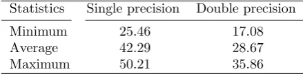
Table 3.7
Statistics ofΛb(k), i.e., memory savings of optimal block configurations against CSR32 in percents, across the tested matrices.
Statistics Single precision Double precision
Minimum 25.46 17.08
Average 42.29 28.67
Maximum 50.21 35.86
the savings were 42.29% and 28.67%, which significantly reduces the amount of data that needs to be transferred between memory and processors during computations.
Table 3.7 shows the statistics of memory savings across all the tested matrices. However, we also wanted to find out which matrices were especially suitable/unsuitable for partitioning in general. For this reason, we measured the memory saving against CSR32 also as a function the following criteria, which are commonly used to distinguish/quantify different types of sparse matrices:
1. application problem type,
2. relative count of matrix nonzero elements (their density),
3. uniformity of the distribution of matrix nonzero elements across its rows.
The application problem types were introduced by Table 2.1. As for the second criterion, we define thedensity
of nonzero elements for anm×nmatrixAwithnnz nonzero elements in percents asϱ(A) =nnz/(m×n)×100. Its values thus ranges from 0 for an empty matrix to 100 to a fully dense matrix.
Letrnnz(i) denote a number of nonzero elements ofith row ofA;rnnz(i) thus ranges from 0 for empty rows to nfor fully dense rows. To allow a collective evaluation of matrices with different row lengths, we transform
rnnz(i) into relative counts in percents as follows: prnnz(i) = rnnz(i)/n×100. The standard deviation of
prnnz(i) fori= 1, . . . , mthen represents an inverse measure of the above introduced third criterion forA. Zero standard deviation ofprnnz(i) then implies a matrix whose all rows have exactly the same number of nonzero elements.
Recall that in Section 2 we defined two kinds of the numbers of nonzero elements, counting either all of them or just those stored in a computer memory (for unsymmetric matrices, these numbers would be equal). Accordingly, we can quantify the above introduced second and third matrix criteria in two ways; we further show results for both of them.
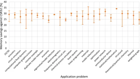
The measurements for the first criterion and double precision are presented by Table 3.2; the results for single precision are practically the same, just scaled accordingly. We need to be careful when making general conclusions based on these results, since for some problem types, our tested suite of matrices contain only few representatives. However, we may observe that the memory savings against CSR32 were relatively consistent across problem types; there was no problem type that would provide much better or much worse savings than the others, including even the graph matrices.
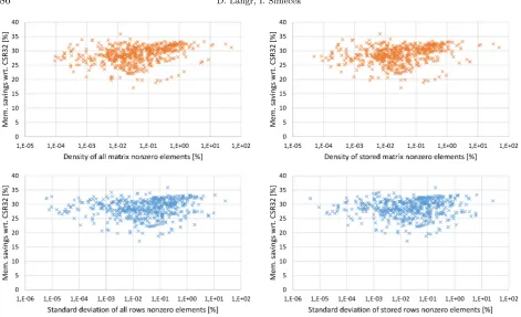
The measurements for the second and third criteria are presented by the top and bottom parts of Table 3.3, respectively. Again, we show results only for double precision for the same reason as above. Seemingly (and maybe interestingly), there is no obvious correlation between the memory savings of partitioned matrices against CSR32 and the density of nonzero elements of matrices / uniformity of their distribution across matrix rows.
In summary, the obtained results support the potential profitability of partitioning of sparse matrices in general.
3.8. Memory Savings Against Index-Compressed CSR. Recall that within our block approach we assumed index compression, i.e., a minimum amount of bits to be used for all indices (Table 2.4). However, for CSR32, we considered all indices to occupy 32 bits each, since this is the most common implementation of CSR in practice. To provide fair comparison with CSR, we therefore also considered storage of matrices in the implementation of CSR with indexed compressed indices; we call such a variant CSRic.
0 5 10 15 20 25 30 35 40
Me
m
o
ry
s
a
v
in
g
s
a
g
a
in
st
C
S
R
3
2
[
%
]
Application problem
Fig. 3.2. Statistics of relative memory savings against CSR32 in percents across the tested matrices grouped by individual problem types, measured for double precision. Circles represent average values, the extents from minimal to maximal values are indicated by bars.
Table 3.8
Statistics ofΩb(k), i.e., memory savings of optimal block configurations against CSRic in percents, across the tested matrices.
Statistics Single precision Double precision
Minimum 1.41 0.84
Average 22.43 13.70
Maximum 35.63 22.43
a precision given byb. The function
Ωb(k) = (
1−min {
MMF⊞(Ak, s, h×w, b) :s∈ S6, h×w∈ B64} MMFCSRic(Ak, b)
)
×100 (3.7)
then expresses how much memory in percents we would save if we stored the tested matrix Ak in its optimal block configuration instead of in CSRic. We measured these memory savings for all the tested matrices and processed them statistically; the results are presented by Table 3.8. Memory footprints of matrices stored in CSRic are either the same or more likely lower than memory footprints of matrices stored in CSR32. Therefore, memory savings Ωb(k) are lower than Λb(k). However, even when compared to CSRic, our block approach still reduces memory footprints of matrices in average by 22.43% and 13.70% for single and double precision, respectively, which represents significant memory savings.
Fig. 3.3.Relative memory savings against CSR32 in percents as a function ofϱ(above) and the standard deviation of prnnz (below) measured for the tested matrices and double precision considering both all/stored nonzero elements.
On the contrary, if we do not assume any particular structure of nonzero elements, we can find an amount of memory required to store the information about matrix nonzero structure as follows: nnz nonzero elements can be placed tom×npositions in C(mn,nnz) different ways, where
C(mn,nnz) = (mn)!
(mn−nnz)!·nnz!. (3.8)
To distinguish between them, we thus need log2C(mn,nnz) bits. Such an approach is employed by so-called
Entropy based format(EBF) [30], which is rather a theoretical concept and establishes a lower bound for generic memory footprints of sparse matrices in cases where no assumptions about their structures are made.
Let MMFEBF(A, b) denote a memory footprint of a matrixAstored in memory in EBF with respect to a precision given by b. The function
Θb(k) = (
1−min {
MMF⊞(Ak, s, h×w, b) :s∈ S6, h×w∈ B64} MMFEBF(Ak, b)
)
×100 (3.9)
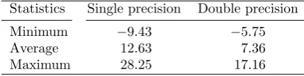
then expresses how much memory in percents we would save if we stored the tested matrix Ak in its optimal block configuration instead of in EBF. We measured these memory savings for all the tested matrices and processed them statistically; the results are presented by Table 3.9. For worst-case matrices, EBF required less memory. However, our block approach still reduced memory footprints of matrices in average by 12.63% and 7.36% for single and double precision, respectively. These results indicate that the nonzero structure of the majority of matrices from our highly diverse benchmark suite have some kind of a block character.
Table 3.9
Statistics ofΘb(k), i.e., memory savings of optimal block configurations against EBF in percents, across the tested matrices.
Statistics Single precision Double precision
Minimum −9.43 −5.75
Average 12.63 7.36
Maximum 28.25 17.16
it is generally worth applying only for special kinds of matrices where nonzero elements contain few unique numbers. To store nnz nonzero elements of a matrixA in memory with respect to a precision given by b, we thus need nnz ×b bits to store their values and some additional space to store the information about their structure. The lower bound for the latter for any particular structure of nonzero elements is 1 bit, since it is sufficient for distinguishing whether or not a matrix has that particular structure. For instance, we can use this bit to indicate whether a matrix is tridiagonal. If it is, the bit would be set and we can store the values of nonzero elements in a dense array; their row and column indices can then be derived from the positions of values in this array. Such an approach can be generally applied for any particular structure of matrix nonzero elements.
In practice, we would need to store in memory also some additional information about a matrix, such as its dimensions or its number of nonzero elements. However, for large matrices such as those from our tested suite, this additional data require a negligible amount of memory, therefore we define a lower bound for a matrix memory footprint simply as MMFlb(A, b) =nnz×b.
Let
Γb ⊞(k) =
( min{
MMF⊞(Ak, s, h×w, b) :s∈ S6, h×w∈ B64} MMFlb(Ak, b)
−1 )
×100. (3.10)
Γb
⊞(k) thus expresses of how much percents is the memory footprint ofAk stored in an optimal block way higher than its lower bound. For comparison purposes, we define corresponding metrics also for CSR32, CSRic, and EBF denoted by Γb
CSR32(k), ΓbCSRic(k), and ΓbEBF(k), respectively:
Γb
CSR32(k) =
(MMF
CSR32(Ak, b) MMFlb(Ak, b)
−1 )
×100, (3.11)
Γb
CSRic(k) =
(MMF
CSRic(Ak, b) MMFlb(Ak, b)
−1 )
×100, (3.12)
Γb
EBF(k) =
(MMF
EBF(Ak, b) MMFlb(Ak, b)
−1 )
×100. (3.13)
The measured statistics of Γb ⊞(k), Γ
b
CSR32(k), ΓbCSRic(k), and ΓbEBF(k) for the tested matrices are shown in Table 3.10. Memory footprints of partitioned sparse matrices were obviously much closer to the lower bounds than memory footprints of matrices stored in CSR32 and CSRic. Namely, they were 5 times closer in average and 2 times in worst cases than CSR32. In best and average cases, they were even significantly closer to the lower bounds than EBF. In best cases, partitioned matrices almost reached their lower-bound memory footprints. For instance, in double precision, 7, 26, and 120 matrices out of 563 provided memory footprints up to 1, 2, and 5 percents above their lower bounds, respectively.
3.11. Best-Case and Worst-Case Matrices. We define abest-case matrix and aworst-case matrix to be a matrix Ak with the lowest and highest value of Γb⊞(k), respectively.
Table 3.10 Statistics ofΓb
⊞(k),ΓbCSR32(k),ΓbCSRic(k), andΓbEBF(k)(in percents) for the tested matrices.
Single precision Double precision
Statistics Blk.-opt. CSR32 CSRic EBF Blk.-opt. CSR32 CSRic EBF
Minimum 0.63 100.02 34.52 6.37 0.31 50.01 17.26 3.18 Average 21.85 111.03 57.22 39.58 10.93 55.51 28.61 19.79 Maximum 71.31 152.39 93.19 67.15 35.66 76.19 46.60 33.58
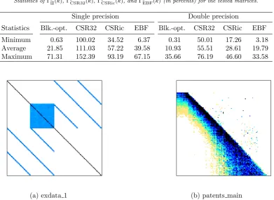
(a) exdata 1 (b) patents main
Fig. 3.4. Visualization of nonzero patterns of the best case (left) and worst case (right) matrices obtained from the UFSMC.
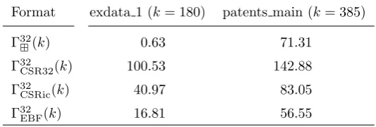
Relative memory footprints for this matrix are shown in Table 3.11. In case of blocking, the memory footprint of this matrix is of only 0.63% higher than its lower bound. In absolute numbers, the lower bound for single precision is 36408000 bits, while the memory footprint for optimal block configuration is 36637064 bits.
The optimal block size for this matrix is 16×16, which results in 5592 nonzero blocks, out of which 4278 blocks are fully dense (have all 256 elements nonzero). Vast majority of the matrix nonzero elements (namely 96.26%) are thus stored in dense blocks, which makes the block approach for storage of this matrix such superior in comparison with other formats. Figure 3.4.a shows that this matrix contains one large dense block where most of its nonzero elements are located.
The optimal block scheme for this matrix is adaptive. The second lowest scheme is bitmap, which provides memory footprint 37890016 bits, i.e., 1.03% higher than the optimum.
3.11.2. Worst-Case Matrix. The worst-case matrix in our benchmark suite wasA385called patents main in the UFSMC. It is a square unsymmetric matrix with 240547 rows/columns and 560943 nonzero elements. Its density ρ(A385) = 9.69e−4%, thus this matrix is of 4 orders of magnitude more sparse than the best-case matrix exdata 1. A visual representation of the matrix is shown in Figure 3.4.b.
Relative memory footprint for this matrix are shown in Table 3.11. In case of blocking, it is significantly higher than the lower bound. In absolute numbers, the lower bound for single precision is 17950176 bits, while the memory footprint for optimal block configuration is 30750736 bits.
Table 3.11
Relative memory footprints of the best case and worst case matrices in percents with respect to their lower bounds, measured for single precision.
Format exdata 1 (k= 180) patents main (k= 385)
Γ32⊞(k) 0.63 71.31
Γ32
CSR32(k) 100.53 142.88
Γ32
CSRic(k) 40.97 83.05
Γ32
EBF(k) 16.81 56.55
memory footprint 31044280, i.e., 9.5e-3% higher than the optimum.
4. Conclusions. Within this study, we analyzed memory footprints of 563 representative sparse matrices with respect to their partitioning into uniformly sized blocks. We considered different block sizes and different ways of storing blocks in a computer memory. The obtained results led us to the following conclusions:
1. Partitioning of sparse matrices substantially reduces memory footprints of sparse matrices when com-pared to the most-commonly used storage format CSR32. The average observed memory savings in case of single and double precision were 42.3 and 28.7 percents of memory space, respectively. The corresponding worst-case savings were 25.5 and 17.1 percents.
2. The corresponding memory savings with respect to index-compressed implementation of CSR, i.e., CSRic, were in case of single and double precision 22.4 and 13.7 percents in average, respectively. The same metric with respect to EBF were 12.6 and 7.4 percents, respectively.
3. Partitioning of sparse matrices provides memory footprints much closer to their lower bounds than CSR32. In average, the measured memory footprints for optimal block configurations were of only 21.9 and 10.9 percents higher than the lower bounds, while the corresponding memory footprints for CSR32 were higher of 111.0 and 55.5 percents. Moreover, the memory footprints of matrices most suitable for block processing approach the lower bounds; the amount of memory required for storing information about the structure of nonzero elements of such matrices is relatively negligible.
4. Partitioning of sparse matrices generally provides memory footprints closer to their lower bound than CSRic and even than EBF. Many sparse matrices in real world contain such form of a structure of nonzero elements that is suitable for block processing.
5. For minimization of memory footprints of partitioned sparse matrices, we cannot consider only a single format for storing blocks. Instead, we need to choose a format according to the structure of matrix nonzero elements either for all its blocks collectively (min-fixed scheme) or for each block separately (adaptive scheme). The latter approach mostly yields lower memory footprints.
6. For minimization of memory footprints of partitioned sparse matrices, we cannot consider only a single block size. However, we can substantially reduce the set of block sizes in the optimization space and still obtain memory footprints close to their optima. In average, the measured memory footprints for the proposed reduced sets of block sizes B20, B14, and B8 and the min-fixed/adaptive schemes were at most of only 1.51 percents higher than the optimal values. Even considering square blocks only is thus generally sufficient for minimization of memory footprints of sparse matrices. However, there exist matrices for which the corresponding metrics are significantly higher and are inversely proportional to the number of tested block sizes. One should thus be aware of whether or not his/her matrices fall into this category and if yes, he/she might consider using larger sets of block sizes.
7. The obtained results seem to be consistent across a wide range of real-world matrices arising from multiple applications problems.
9. We measured memory savings of partitioned sparse matrices against CSR32 as a function of the following criteria, which are frequently used in the literature: the application problem type, the density of matrix nonzero elements, and the standard deviation of the number of nonzero elements across matrix rows. To our best, we did not find any correlation between the memory savings and these criteria; the block approach thus seems reduce memory footprints of sparse matrices in general.
Our findings are encouraging since they show that memory footprints of partitioned sparse matrices can be substantially reduced even when a relatively small block preprocessing optimization space is considered. Whether or not will such a reduction pay off in practice depends on the objective one wants to achieve. A big challenge is to improve the performance of memory-bounded sparse matrix operations due to the reduction of memory footprints of matrices. Within our future work, we plan to face this problem at least partially—we will focus on the development of scalable efficient block preprocessing and SpMV algorithms for the min-fixed and adaptive block storage schemes, and we will evaluate them experimentally on mainstream HPC architectures.
REFERENCES
[1] A. Ashari, N. Sedaghati, J. Eisenlohr, S. Parthasarathy, and P. Sadayappan,Fast sparse matrix-vector multiplica-tion on GPUs for graph applicamultiplica-tions, in Proceedings of the International Conference for High Performance Computing, Networking, Storage and Analysis, SC ’14, Piscataway, NJ, USA, 2014, IEEE Press, pp. 781–792.
[2] R. Barrett, M. Berry, T. F. Chan, J. Demmel, J. Donato, J. Dongarra, V. Eijkhout, R. Pozo, C. Romine, and H. V. der Vorst,Templates for the Solution of Linear Systems: Building Blocks for Iterative Methods, SIAM, Philadelphia, PA, 2nd ed., 1994.
[3] M. Belgin, G. Back, and C. J. Ribbens,Pattern-based sparse matrix representation for memory-efficient SMVM kernels, in Proceedings of the 23rd International Conference on Supercomputing, ICS ’09, New York, NY, USA, 2009, ACM, pp. 100–109.
[4] ,A library for pattern-based sparse matrix vector multiply, International Journal of Parallel Programming, 39 (2011), pp. 62–87.
[5] G. E. Blelloch, M. A. Heroux, and M. Zagha,Segmented operations for sparse matrix computation on vector multipro-cessors, Tech. Rep. CMU-CS-93-173, School of Computer Science, Carnegie Mellon University, 1993.
[6] A. Buluc¸, J. T. Fineman, M. Frigo, J. R. Gilbert, and C. E. Leiserson,Parallel sparse vector and matrix-transpose-vector multiplication using compressed sparse blocks, in Proceedings of the 21st Annual Symposium on Paral-lelism in Algorithms and Architectures, SPAA ’09, New York, NY, USA, 2009, ACM, pp. 233–244.
[7] A. Buluc¸, S. Williams, L. Oliker, and J. Demmel,Reduced-bandwidth multithreaded algorithms for sparse matrix-vector multiplication, in Proceedings of the 2011 IEEE International Parallel & Distributed Processing Symposium, IPDPS ’11, IEEE Computer Society, 2011, pp. 721–733.
[8] D. Buono, F. Petrini, F. Checconi, X. Liu, X. Que, C. Long, and T.-C. Tuan,Optimizing sparse matrix-vector multi-plication for large-scale data analytics, in Proceedings of the 2016 International Conference on Supercomputing, ICS ’16, New York, NY, USA, 2016, ACM, pp. 37:1–37:12.
[9] J.-H. Byun, R. Lin, K. A. Yelick, and J. Demmel,Autotuning sparse matrix-vector multiplication for multicore, Tech. Rep. UCB/EECS-2012-215, EECS Department, University of California, Berkeley, 2012.
[10] J. W. Choi, A. Singh, and R. W. Vuduc,Model-driven autotuning of sparse matrix-vector multiply on GPUs, in Proceedings of the 15th ACM SIGPLAN Symposium on Principles and Practice of Parallel Programming, PPoPP ’10, New York, NY, USA, 2010, ACM, pp. 115–126.
[11] T. A. Davis and Y. F. Hu,The University of Florida Sparse Matrix Collection, ACM Transactions on Mathematical Software, 38 (2011), pp. 1:1–1:25.
[12] J. Dongarra,Preface: Basic linear algebra subprograms technical (BLAST) forum standard, International Journal of High Performance Computing Applications, 16 (2002), p. 1.
[13] R. Eberhardt and M. Hoemmen, Optimization of block sparse matrix-vector multiplication on shared-memory parallel architectures, in Proceedings of the 2016 IEEE International Parallel and Distributed Processing Symposium Workshops (IPDPSW), 2016, pp. 663–672.
[14] G. Goumas, K. Kourtis, N. Anastopoulos, V. Karakasis, and N. Koziris,Performance evaluation of the sparse matrix-vector multiplication on modern architectures, The Journal of Supercomputing, 50 (2009), pp. 36–77.
[15] IEEE Standard for Floating-Point Arithmetic, IEEE Std 754-2008, (2008), pp. 1–58.
[16] E.-J. Im and K. Yelick,Optimizing sparse matrix computations for register reuse in SPARSITY, in Proceedings of the International Conference on Computational Science (ICCS 2001), Part I, vol. 2073 of Lecture Notes in Computer Science, Springer Berlin Heidelberg, 2001, pp. 127–136.
[17] E.-J. Im, K. Yelick, and R. Vuduc,Sparsity: Optimization framework for sparse matrix kernels, International Journal of High Performance Computing Applications, 18 (2004), pp. 135–158.
[18] R. Kannan,Efficient sparse matrix multiple-vector multiplication using a bitmapped format, in 20th Annual International Conference on High Performance Computing, 2013, pp. 286–294.
vol. 1, Aug 2009, pp. 247–256.
[20] D. Langr,Algorithms and Data Structures for Very Large Sparse Matrices, PhD thesis, Czech Technical University in Prague, 2014.
[21] D. Langr and I. ˇSimeˇcek,On memory footprints of partitioned sparse matrices, in Proceedings of the Federated Conference on Computer Science and Information Systems (FedCSIS 2017), vol. 11 of Annals of Computer Science and Information Systems, Polish Information Processing Society, 2017, pp. 513–512.
[22] D. Langr, I. ˇSimeˇcek, and T. Dytrych,Block iterators for sparse matrices, in Proceedings of the Federated Conference on Computer Science and Information Systems (FedCSIS 2016), IEEE Xplore Digital Library, 2016, pp. 695–704.
[23] D. Langr, I. ˇSimeˇcek, and P. Tvrd´ık,Storing sparse matrices in the adaptive-blocking hierarchical storage format, in Proceedings of the Federated Conference on Computer Science and Information Systems (FedCSIS 2013), IEEE Xplore Digital Library, 2013, pp. 479–486.
[24] D. Langr, I. ˇSimeˇcek, P. Tvrd´ık, T. Dytrych, and J. P. Draayer, Adaptive-blocking hierarchical storage format for sparse matrices, in Proceedings of the Federated Conference on Computer Science and Information Systems (FedCSIS 2012), IEEE Xplore Digital Library, 2012, pp. 545–551.
[25] D. Langr and P. Tvrd´ık,Evaluation criteria for sparse matrix storage formats, IEEE Transactions on Parallel and Dis-tributed Systems, 27 (2016), pp. 428–440.
[26] Morton,A computer oriented geodetic data base and a new technique in file sequencing, Tech. Rep. Ottawa, Canada, IBM Ltd., 1966.
[27] R. Nishtala, R. W. Vuduc, J. W. Demmel, and K. A. Yelick,Performance modeling and analysis of cache blocking in sparse matrix vector multiply, Tech. Rep. UCB/CSD-04-1335, Computer Science Division (EECS), University of California, 2004.
[28] R. Nishtala, R. W. Vuduc, J. W. Demmel, and K. A. Yelick,When cache blocking of sparse matrix vector multiply works and why, Applicable Algebra in Engineering, Communication and Computing, 18 (2007), pp. 297–311.
[29] I. ˇSimeˇcek and D. Langr,Space and execution efficient formats for modern processor architectures, in Proceedings of the 17th International Symposium on Symbolic and Numeric Algorithms for Scientific Computing (SYNASC 2015), IEEE Computer Society, 2015, pp. 98–105.
[30] I. ˇSimeˇcek, D. Langr, and P. Tvrd´ık, Space-efficient sparse matrix storage formats for massively parallel systems, in Proceedings of the 14th IEEE International Conference of High Performance Computing and Communications (HPCC 2012), IEEE Computer Society, 2012, pp. 54–60.
[31] F. S. Smailbegovic, G. N. Gaydadjiev, and S. Vassiliadis, Sparse Matrix Storage Format, in Proceedings of the 16th Annual Workshop on Circuits, Systems and Signal Processing, ProRisc 2005, 2005, pp. 445–448.
[32] P. Stathis, S. Vassiliadis, and S. Cotofana,A hierarchical sparse matrix storage format for vector processors, in Proceed-ings of the 17th International Symposium on Parallel and Distributed Processing, IPDPS ’03, Washington, DC, USA, 2003, IEEE Computer Society, p. 61.
[33] Y. Tao, Y. Deng, S. Mu, Z. Zhang, M. Zhu, L. Xiao, and L. Ruan,GPU accelerated sparse matrix-vector multiplication and sparse matrix-transpose vector multiplication, Concurrency and Computation: Practice and Experience, (2014). [34] P. Tvrd´ık and I. ˇSimeˇcek,A new diagonal blocking format and model of cache behavior for sparse matrices, in Proceedings
of the 6th International Conference on Parallel Processing and Applied Mathematics (PPAM 2005), vol. 3911 of Lecture Notes in Computer Science, Springer Berlin Heidelberg, 2006, pp. 164–171.
[35] S. Williams, A. Waterman, and D. Patterson,Roofline: An insightful visual performance model for multicore architec-tures, Commun. ACM, 52 (2009), pp. 65–76.
[36] X. Yang, S. Parthasarathy, and P. Sadayappan, Fast sparse matrix-vector multiplication on GPUs: Implications for graph mining, Proc. VLDB Endow., 4 (2011), pp. 231–242.
Edited by: Sasko Ristov
Received: Feb 8, 2018