COMPARISON OF ACCURACY PREDICTION INDONESIAN STOCK
EXCHANGE (IDX) WITH ARIMA, ARCH AND GARCH METHODS
1Yunita Dahlan, 2Masyhuri Hamidi
1Master’s Student, 2Lecture, Department Masters of Management Faculty of Economic, Andalas University, Padang City, West Sumatera, Indonesia.
Email – 1 [email protected]
1. INTRODUCTION:
Now in Indonesia the "Yuk Nabung Saham" movement has been launched by the government and the Indonesia Stock Exchange. How to get shares can also be made online by opening an account at a securities company that is an Indonesian broker. This makes the capital market more developed because access to invest in the capital market is easier, wherever and whenever investors are able to conduct stock transactions.
Movements in the capital market are closely related to the activities of investors who invest in the capital market. For an investor, it is very necessary to know the investment movements that are happening or in the future. This momentum can be used by investors to prepare an accurate strategy in investing so that they will get maximum profit. But on average investors cannot read the moment of increase and decrease in the value of the IDX appropriately, so that many investors actually get small profits or even experience losses due to misinterpretations of the IDX. Investors need predictors that can assist in making investment decisions, so forecasting methods will be needed.
Rode (1995) argues that there are no perfect indicators that can be used as guidelines in investing. This makes analysts still looking for the latest indicators that will be used as a guide in investing. One indicator that is often used to predict is the Autoregressive Integrated Moving Average (ARIMA) and ARCH/GARCH.
Whereas the phenomenon that can be seen in the last five years where the exchange rate of rupiah against foreign money has weakened to penetrate above Rp. 15,000, the change in the reference rate of the BI Rate becomes BI 7-Day Repo Rate making me interested in trying to do research again in predicting IDX movement with two approaches, namely ARIMA method approach and ARCH / GARCH method approach, as well as trying to prove the accuracy of the ARIMA method and ARCH / GARCH method in predicting IDX price movements using data in 2014-2018, and proving whether the ARIMA method is still more accurate than the ARCH method / GARCH in conditions where the weakening rupiah exchange rate and the rise of Indonesian interest rates in a row. Based on this description the authors are interested in conducting research on which method is the most accurate for predicting the Composite Stock Price
Index by taking the title "Comparison of Accuracy of Prediction of the Composite Stock Price Index with the
ARIMA, ARCH / GARCH".
From the description of the background, the problems can be formulated as follows: 1. Is the ARIMA, ARCH / GARCH method able to predict the Composite Stock Price Index?
2. Which of the ARIMA, ARCH / GARCH is more accurate in predicting the Composite Stock Price Index?
The objectives of this study are as follows:
1. To prove the accuracy of the ARIMA, ARCH / GARCH method in predicting the Composite Stock Price Index in the future.
2. To compare the accuracy of the ARIMA, ARCH / GARCH method in predicting the Composite Stock Price Index in the future.
Abstract: This study aims to examine the effect of exchange rate and interest rates on the movement of the Composite Stock Price Index using the causality method and pattern approach. The pattern approach method predicts the movement of the stock price index through the movement pattern itself like the ARIMA method while the causality method predicts the movement of the stock price index through the variables that influence it such as the ARCH and GARCH methods. This study was conducted using monthly IHSG data, exchange rates and interest rates as of January 2014 to November 2018. From the results of the study it can be concluded that the exchange rate does not significantly influence the IDX value while the interest rate has a significant effect on the IDX, but the exchange rates and interest rates together the same has a significant negative effect on the value of the IDX. And after the two methods were compared the results were obtained that the ARIMA method gave more accurate
predictive results in predicting the IHSG movement:
Monthly, Peer-Reviewed, Refereed, Indexed Journal Impact Factor: 4.526 Publication Date: 31/01/2019
2. METHOD:
Data uses two forecasting models, namely ARIMA, ARCH and GARCH models.
A. ARIMA Model
By using the Box Jenkins method, there are steps as follows: 1. Stationary Test
(1) Corelogram is the technique of stationary time series data identification through the Autocorrelation (ACF) function. This function is useful for explaining a stochastic process, and will provide information on how the correlation between data (Yt) is adjacent.
(2) Root Test Unit developed by Dickey-Fuller as the Augmented Dickey-Fuller (ADF) Test. Test with the E views program with the following hypothesis:
Ho: There is a root unit; Ha: There is no unit root
Criteria: Reject Ho if the ADF test statistic value is <critical value, meaning that the data has a root unit or not stationary or the model becomes a random walk.
2. Identification
This step seeks and determines p, d, and q with the help of the autocorrelation corelogram (ACF) for the order (q - MA) which measures the correlation between observations with the lag and partial autocorrelation corelogram (PACF) for the order (p-AR) measure correlation between observations with the lag and by controlling the correlation between the two observations with lags less than k.
3. Estimates
After going through the trial and error ARIMA model, a significant model was chosen and Akaike Criterion, Schwartz the smallest criterion and parsimony were chosen.
4. Diagnostic Test
diagnostic test can be performed to ensure that the model specifications are correct. If the residual turns out to be white noise, it means that the model is good.
5. Test whether ACF and PACF are significant. If ACF and PACF are not significant, this is an indication that the residual is white noise, meaning the model is appropriate.
6. Prediction, made after the model passes the diagnostic test. So that we can determine the conditions to come.
B. ARCH and GARCH models
This model can be used provided that the data has heteroscedasticity by testing the ARCH effect introduced by Robert Engle, which can be done with the following steps:
a. Regression between dependent and independent variables. b. ARCH LM test of the residue from regression point a. With the hypothesis:
H0 = α0 = α1 = 0 (There is no ARCH Effect)
H1 = α0 α1 ≠ 0 (There is an ARCH Effect)
If there is an ARCH Effect, continue testing by adding lag until there is no ARCH Effect anymore. Then Analysis of Results (Proof of Hypothesis) and Prediction. After obtaining the best model based on the smallest Akaike Info Creterion (AIC), and the model fulfilling the BLUE (Best Linear Unbiased Estimator) criteria, the results analysis and forecasting can be done.
1. Robert Engle's model for ARCH and GARCH equations
Equations of ARCH (p) and GARCH (p, q) Models - Robert Engle
ARCH (p) σt2 = α0 + Σ αie2t-1 (1)
GARCH (p, q) σt2 = α0 + Σ αie2t-1 + Σ λiσqt-1 (2)
Information:
Σt = var (et) is a residual variant as a function of past volatility and residual variants. Described by two components. Variable α0 = constant
Variable αie2t-1 = component ARCH (p)
γ = Parameters
σqt = T-variant
This model appears with the aim of overcoming the greater number of p, so that the more parameters that have to be estimated can result in the precision of the estimator decreasing (often found in daily analysis data). So that the
With the equation the error variant is
σt2 = α0 + α1 e2t-1 + λ1 σ2t-1 (4)
Yi = Dependent variable (past JCI closing) b0 = Constants
b1 = Coefficient of model
X1 = Independent variable (Exchange Rate and Interest)
σt2 = Variant error
e2t-1 = error / residual / volatility in period-1
σ2t-1 = Period t-1 error variant
3. ANALYSIS:
Variabel
a. Composite Stock Price Index (IDX)
IDX is an indicator that displays the condition of the stock market based on its movements both during active and passive market conditions that show the combined performance of all shares listed on the stock exchange so that it can influence investment decisions. The data used is the monthly value of the IDX closing 30 January 2014 - 30 November 2018.
b. Exchange rate
Exchange rate is the price of the exchange rate of a country's currency against the price of the exchange rate of another country's currency. In this study the exchange rate used to be measured is the monthly value of the US Dollar against the Rupiah period 30 January 2014 - 30 November 2018.
c. Interest rate
The interest rate is the monetary policy set by Bank Indonesia which is the price of the loan. Interest rates are expressed as a percentage of money from the principal per unit of time which is used as a benchmark by commercial banks to determine loan interest rates and loan interest rates. The data used in this study is the monthly interest rate data for the period 30 January 2014 - 30 November 2018.
A. Method ARIMA 1. IDX
a) Normalitas Test
0 2 4 6 8 10 12 14 16
-0.08 -0.06 -0.04 -0.02 0.00 0.02 0.04 0.06
Series: Residuals Sample 2 59 Observations 58
Mean 9.11e-13 Median 0.004870 Maximum 0.066556 Minimum -0.084727 Std. Dev. 0.030626 Skewness -0.960235 Kurtosis 4.016901
Jarque-Bera 11.41220 Probability 0.003326
Jarque-Bera Test
Probability of the Jarque-Bera IDX is 0.003326, which means that the probability of this outcome is smaller than 0.05 so that the data in the study are not normally distributed. However, further stages of data processing can still be implemented because in the ARIMA time series testing does not have to meet the assumptions of normality of data (Winarno, 2012).
Monthly, Peer-Reviewed, Refereed, Indexed Journal Impact Factor: 4.526 Publication Date: 31/01/2019
Correlogram Actual IDX Differencing Orde 1
c) Identification.
From the results of the table above it can be seen that the autocorrelation and partial autocorrelation values are getting closer to zero as the lag value increases. The table above shows "white noise" or "pure random".
d) Estimates
Tabel 1 Estimates
Information Coeffisien t-hit Prob
Model AR
Constanta 8,651941 106,7625 0.0000
AR(1) 0,938089 24,71396 0.0000
Model MA
Constanta 8,577102 552,9604 0.0000
MA(1) 0,829092 11,19901 0.0000
The auto regressive integreted (AR) model and the moving average (MA) can be seen as predictive variables given the code AR (1) and MA has a coefficient value positive with 0.938 and 0.829. the prediction model is stated precisely because the resulting probability value is below 95% confident level, from the model it is predicted that JCI in the future will be strengthened.
e) Diagnostic Test.
Tabel 2 Diagnostic
Model AIC SBC SSE Adj
R-Square
AR(1) -4,085 -4,014 0,053 0.915
MA(1) -2,588 -2,517 0,243 0.631
Based on the comparison of the AR (1) and MA (1) models, it appears that each of them is good enough to be used but the AR (1) model is considered more appropriate because it has an adjusted R-square value obtained far above the MA model (1), Sum coefficient value Square resid (SSE) AR (1) which is much smaller than SSE MA (1), but the Akaike info criterion (AIC) and Schawarz Criterion values are smaller AR (1) than MA (1), thus it can be concluded that the chosen model is AR (1).
2. Exchange Rate
0 2 4 6 8 10 12
-0.06 -0.04 -0.02 0.00 0.02 0.04
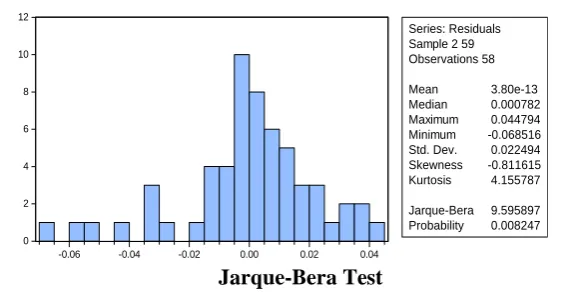
Series: Residuals Sample 2 59 Observations 58
Mean 3.80e-13 Median 0.000782 Maximum 0.044794 Minimum -0.068516 Std. Dev. 0.022494 Skewness -0.811615 Kurtosis 4.155787
Jarque-Bera 9.595897 Probability 0.008247
Jarque-Bera Test
in the table above, it can be seen that probability Jarque Bera exchange rate is 0.008247 which means that the results of this probability are smaller than 0.05 so the data in the study are not normally distributed.
b) Stationary test
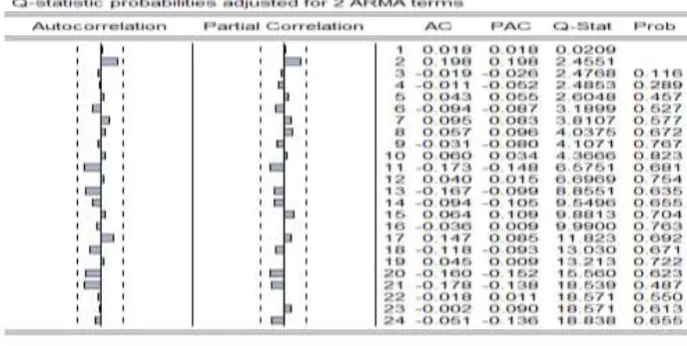
Correlogram Actual Exchange rate Differencing Orde 1
c) Identification.
From the results of the table above it can be seen that the autocorrelation and partial autocorrelation values are getting closer to zero as the lag value increases. The table above shows "white noise" or "pure random".
d) Estimates
Tabel 3 Estimates
Information Coeffisien t-hit Prob
Model AR
Constanta 9,532704 162,7986 0.0000
AR(1) 0,937176 20,12163 0.0000
Model MA
Constanta 9,490392 970,2962 0.0000
MA(1) 0,755415 8.474486 0.0000
Based on the exchange forecasting model with the AR model (1) it is known that the tendency to depreciate the Rupiah exchange rate in the future will still occur, this is evidenced by the AR predictor coefficient value (1) which is positive at 0.937, the same is seen in the MA historical data coefficient comparison (1 ) which is also positive, which is equal to 0.755. In accordance with the results of the test, it is also seen that the probability value is below 0.05 so that it can be concluded that the ARIMA model formed is appropriate or feasible to use..
e) Diagnostic Test
Tabel 4 Estimates
Model AIC SBC SSE Adj
Monthly, Peer-Reviewed, Refereed, Indexed Journal Impact Factor: 4.526 Publication Date: 31/01/2019
AR(1) -4,648 -4,577 0,030 0.876
MA(1) -3,426 -3,356 0,105 0.584
Based on the comparison of AR (1) and MA (1) models, it appears that each of them is right enough to be used, but the AR (1) model is considered more appropriate because it has an adjusted R-square value that is obtained far above the MA model (1), Sum Square resid (SSE) coefficient value (1) which is much smaller than SSE MA (1), but Akaike info criterion (AIC) and Schawarz Criterion values are smaller AR (1) than MA (1), thus it can be concluded that the chosen model is AR (1).
3. Interest Rate
a) Normalitas Test
0 4 8 12 16 20 24 28
-0.010 -0.005 0.000 0.005
Series: Residuals Sample 2 58 Observations 57
Mean -1.57e-06 Median 0.000282 Maximum 0.004854 Minimum -0.012288 Std. Dev. 0.002131 Skewness -3.150556 Kurtosis 21.08386
Jarque-Bera 870.9835 Probability 0.000000
Jarque-Bera Test
Based on the test results as shown in Table, it can be seen that the probability of Jarque-Bera interest rate is 0.000000, which means that the results of this probability are smaller than 0.05 so that the data in the study are not normally distributed.
b) Stationery test
Correlogram Actual Interest rate Differencing Orde 1
c) Identification.
From the results of the table above it can be seen that the autocorrelation and partial autocorrelation values are getting closer to zero as the lag value increases. The table above shows "white noise" or "pure random".
d) Estimates
Tabel 5 Estimates
Information Coeffisien t-hit Prob
Model AR
Constanta 0,049607 2.757 0.0079
AR(1) 0,978349 45.502 0.0000
Model MA
Constanta 0.061446 32,78684 0.0000
Based on the interest rate forecasting model with the AR model (1) it is known that the central bank's tendency to raise interest rates in the future as it did in the past will continue to occur considering that in the regression coefficient model the two prediction models are positive. In the test results it is seen that both probability AR (1) and MA (1) have the same probability value of 0,000 which is far below the error level of 0.05 so that it can be concluded that the AR (1) and MA (1) models are the right models.
e) Diagnostic Test
Tabel 6 Diagnostic
Model AIC SBC SSE Adj
R-Square
AR(1) -9.339 -9.268 0.000279 0.973
MA(1) -6.920 -6.850 0.003188 0.699
Based on the comparison of the AR (1) and MA (1) models, it appears that each of them is good enough to be used but the AR (1) model is considered more appropriate because it has an adjusted R-square value obtained far above the MA model (1), Sum coefficient value Square resid (SSE) AR (1) which is much smaller than SSE MA (1), but the Akaike info criterion (AIC) and Schawarz Criterion values are smaller AR (1) than MA (1), thus it can be concluded that the chosen model is AR (1).
-.12 -.08 -.04 .00 .04 .08
8.3 8.4 8.5 8.6 8.7 8.8 8.9
5 10 15 20 25 30 35 40 45 50 55
Residual Actual Fitted
Forecasting
From the picture above, it can be seen that the red line shows the actual JCI line and the green line shows the forecasting of the JCI value in the future where the graph lines are quite coincide with each other means that the forecasting results are close to the actual value.
B. ARCH/GARCH
a) Analysis ARCH
Tabel 7
Goodness of Fit ARCH C(1)*Exchange rate & Interest RateSBI IDX
Keterangan Koefisien t-hit Prob
Model C(1)*KURS IHSG
C(1) * KURS 0.903613 640,0689 0.000
Model C(1)*SBI IHSG
C(1)*SBI 0,6877 33,11413 0.000
Monthly, Peer-Reviewed, Refereed, Indexed Journal Impact Factor: 4.526 Publication Date: 31/01/2019
Based on the Autoregressive Conditional Heteroscedasticity analysis, it can be seen from the regression coefficient value of variable C (1) * Exchange Rate which is positive at 0.903613. The coefficient value shows that changes in exchange rates tend to strengthen (appreciate), so that it will spur growth in investment in the country and encourage the strengthening of the Composite Stock Price Index to reach 0.903613 times. The prediction rate is supported by a probability value of 0,000. Given the stages of data processing carried out using an error rate of 0.05. Then the probability value of 0.000 <alpha 0.05, the tendency for appreciation or strengthening of the Rupiah exchange rate in the future will encourage higher IDX growth in the future.
In the second equation model using the variable C (1) * Interest rate which is calculated by the IDX, the interest rate trend observed from the regression coefficient slope shows a positive result of 0.6877. The results obtained show that Bank Indonesia is predicted to continue to increase interest rates to maintain monetary stability, although interest rates continue to increase the trend of changes in the IDX is relatively increasing in the future. This is reinforced by a probability value of 0,000 which has been far below the error rate of 0.05, so it can be concluded that changes in the increase in central bank interest rates will encourage a stronger composite share price index in the future.
b) Analysis GARCH
Tabel 8
Estimate Generalized Autoregressive Conditional Heteroscedasticity (GARCH) Variabel
Exchange Rate
Coeffisien -0,037992
Probability 0,5884
Resid(-1)^2 1,612249
Probability 0,0433
Interest Rate
Coeffisien -7,440740
Probability 0,0000
GARCH(-1) -0,159721
Probability 0,0003
R-square 0,592458
C 9,381077
IDX= 9,381077 – 0,37992Exchange Rate – 7,440740Interest Rate
In accordance with the data processing, it can be seen that the coefficient of determination produced is equal to 0.592, the results obtained show that the exchange rate and interest rates of Bank Indonesia have a variety of contributions in influencing JCI changes by 59.24% while the remaining 40.76% is explained by other variables that do not used in the current research model. In accordance with the results of data processing that has been done, it can be seen that the exchange rate variable has a regression coefficient marked negative at -0.37992. The results obtained are strengthened by a probability value of 0.5844. Data processing is carried out using an error rate of 0.05. The results obtained show that the probability value of 0.5844 is above the error level of 0.05, so the decision can be concluded that the exchange rate has a negative and not significant effect on the composite stock price index on the Indonesia Stock Exchange.
In the risk estimation model, the residual coefficient value is 1.612249, the results obtained show that the exchange rate change is expressed as a risk that can affect the increase in the JCI, the estimated value is significant because the probability value generated in the model is 0.0433. The results obtained are below 0.05. It means that exchange rate risk will affect the JCI in the future. At the data processing stage, it can also be seen that the variable interest rate of Bank Indonesia has a negative regression coefficient of -7.440740. The results obtained are strengthened with a probability value of 0,000. The stages of data processing are carried out using an error rate of 0.05. The results obtained show that the probability value of 0,000 is below the error level of 0.05, the decision is that Ho is rejected and Ha is accepted so it can be concluded that the interest rate of Bank Indonesia has a negative and significant effect on the composite stock price index on the Indonesia Stock Exchange.
0.05, thus it can be concluded that Bank Indonesia's policy to increase the interest rate will reduce the value of securities investments, especially stocks, thus encouraging the correction of the Composite Stock Price Index in the future.
-.15 -.10 -.05 .00 .05 .10 .15 .20
8.3 8.4 8.5 8.6 8.7 8.8 8.9
5 10 15 20 25 30 35 40 45 50 55
Residual Actual Fitted
Forecasting
From the picture above, it can be seen that the red line shows the actual IDX line and the green line shows the forecasting of the IDX value in the future where the graph lines are quite coincide with each other means that the forecasting results are close to the actual value.
The comparison of IHSG prediction results using the ARIMA, ARCH and GARCH methods was obtained that the ARIMA method is different from the ARCH / GARCH method and the ARIMA method is considered a more accurate method because from the comparison of forecasting graph results between ARIMA, ARCH and GARCH methods ARIMA forecasting line is closer actual value compared to ARCH and GARCH forecasting charts in predicting IDX.
5. CONCLUSION:
o The second test results using the ARIMA method shows that the IDX variable data, the exchange rate and interest
rates are not stationary, while the requirements of the ARIMA method are data must be stationary, differencing processes are carried out. After transformation, the data can be stationary and the ARIMA test can be continued. IDX variables, exchange rates and interest rates modeled in ARIMA obtain significant and diagnostic test results that are significant, meaning that there is a very strong relationship between current period data and previous period.
o The third test result using the ARCH / GARCH method shows that the independent variable namely the exchange
rate does not have a significant effect on the IDX where it has a significant number of 0.05884, the value is greater than the significance level of 5% (0.05884> 0.05), while the interest rate variable has a significant influence on the IDX where it has a significant number of 0.0000, its value is smaller than the significance level of 5% (0.0000 <0.05). However, when viewed in the GARCH test, it means that the exchange rate and interest rates together have an influence on the IDX, which is equal to 59.24%, and the remaining 40.76% is influenced by other factors outside the research variable.
And from the results of these methods, it is found that the ARIMA, ARCH and GARCH methods are different and the ARIMA method provides predictions that tend to be more accurate than the ARCH / GARCH method because the ARIMA method forecasting graph results are closer to the actual IDX.
REFERENCES:
1. Ernayani, Rihfenti. 2015. Pengaruh Kurs Dolar, Indeks Dow Jones Dan Tingkat Suku Bunga SBI Terhadap
IHSG, Juranl Sains Terapan. Vol. 1. No. 2. ISSN: 2406-8810.
2. Fikri & Andini. 2012. Pengaruh Volume Perdagangan Saham, Nilai Tukar Dan Indeks Hang Seng Terhadap
Pergerakan Indeks Harga Saham Gabungan. Jurnal Akuntansi & Bisnis. Vol. 7. No. 2.
3. Grestandhi, Jordan dkk. 2011. Analisis Perbandingan Metode Peramalan Indeks Harga Saham Gabungan (IHSG) Dengan Metode Ols-Arch/GARCH dan Arima, Jurnal Matematika FSM UKSW, ISBN: 978-979-16353-6-3.
4. Murni, Asfia. 2013. Ekonomika Makro. Edisi Revisi. Bandung : PT. Refika Aditama Anoraga, Pandji dan Piji