Parallel Vector Field Embedding

Parallel Vector Field Embedding

Binbin Lin BINBINLIN@ZJU.EDU.CN

Xiaofei He XIAOFEIHE@CAD.ZJU.EDU.CN

Chiyuan Zhang PLUSKID@GMAIL.COM

State Key Lab of CAD&CG College of Computer Science Zhejiang University

Hangzhou, 310058, China

Ming Ji MINGJI1@ILLINOIS.EDU

Department of Computer Science

University of Illinois at Urbana Champaign Urbana, IL 61801, USA

Editor:Mikhail Belkin

Abstract

We propose a novel local isometry based dimensionality reduction method from the perspective of vector fields, which is called parallel vector field embedding (PFE). We first give a discussion on local isometry and global isometry to show the intrinsic connection between parallel vector fields and isometry. The problem of finding an isometry turns out to be equivalent to finding orthonormal parallel vector fields on the data manifold. Therefore, we first find orthonormal parallel vector fields by solving a variational problem on the manifold. Then each embedding function can be obtained by requiring its gradient field to be as close to the corresponding parallel vector field as possible. Theoretical results show that our method can precisely recover the manifold if it is isometric to a connected open subset of Euclidean space. Both synthetic and real data examples demonstrate the effectiveness of our method even if there is heavy noise and high curvature.

Keywords: manifold learning, isometry, vector field, covariant derivative, out-of-sample extension

1. Introduction

In many data analysis tasks, one is often confronted with very high dimensional data. There is a strong intuition that the data may have a lower dimensional intrinsic representation. Various re-searchers have considered the case when the data is sampled from a submanifold embedded in much higher dimensional Euclidean space. Consequently, estimating and extracting the low dimensional manifold structure, or specifically the intrinsic topological and geometrical properties of the data manifold, become a crucial problem. These problems are often referred to as manifold learning (Belkin and Niyogi, 2007).

has maximum variance. However, these linear methods may fail to recover the intrinsic manifold structure when the data manifold is not a low dimensional subspace or an affine manifold.

There are various works on nonlinear dimensionality reduction in the last decade. The typical work includes isomap (Tenenbaum et al., 2000), locally linear embedding (LLE, Roweis and Saul, 2000), Laplacian eigenmaps (LE, Belkin and Niyogi, 2001), Hessian eigenmaps (HLLE, Donoho and Grimes, 2003) and diffusion maps (Coifman and Lafon, 2006; Lafon and Lee, 2006; Nadler et al., 2006). Isomap generalizes MDS to the nonlinear manifold case which tries to preserve pair-wise geodesic distances on the data manifold. Diffusion maps tries to preserve another meaningful distance, that is, diffusion distance on the manifold. Isomap is an instance of global isometry based dimensionality reduction techniques, which tries to preserve the distance function or the metric of the manifold globally. One limitation of Isomap is that it requires the manifold to be geodesically convex. HLLE is based on local isometry criterion, which successfully overcomes this problem. Laplacian operator and Hessian operator are two of the most important differential operators in manifold learning. Intuitively, Laplacian measures the smoothness of the functions, while Hessian measures how a function changes the metric of the manifold. However, the Laplacian based meth-ods like LLE and LE mainly focus on the smoothness of the embedding function, which may not be an isometry. The major difficulty in Hessian based methods is that they have to estimate the second order derivative of embedding functions, and consequently they have strong requirement on data samples.

One natural nonlinear extension of PCA is kernel principal component analysis (kernel PCA, Sch¨olkopf et al., 1998). Interestingly, Ham et al. (2004) showed that Isomap, LLE and LE are all special cases of kernel PCA with specific kernels. Recently, Maximum Variance Unfolding (MVU, Weinberger et al., 2004) is proposed to learn a kernel matrix that preserves pairwise distances on the manifold. MVU can be thought of as an instance of local isometry with additional consideration that the distances between two points that are not neighbors are maximized.

Tangent space based methods have also received considerable interest recently, such as local tangent space alignment (LTSA, Zhang and Zha, 2004), manifold charting (Brand, 2003), Rieman-nian Manifold Learning (RML, Lin and Zha, 2008) and locally smooth manifold learning (LSML, Doll´ar et al., 2007). These methods try to find coordinates representation for curved manifolds. LTSA tries to construct a global coordinate via local tangent space alignment. Manifold charting has a similar strategy, which tries to expand the manifold by splicing local charts. RML uses normal coordinate to unfold the manifold, which aims to preserve the metric of the manifold. LSML tries to learn smooth tangent spaces of the manifold by proposing a smoothness regularization term of tangent spaces. Vector diffusion maps (VDM, Singer and Wu, 2011) is a much recent work which considers the tangent spaces structure of the manifold to define and preserve the vector diffusion distance.

of embedding functions preserves the metric of the manifold. As pointed out by Goldberg et al. (2008), almost all spectral methods including LLE, LE, LTSA and HLLE use global normalization for embedding, which sacrifices isometry. PFE overcomes this problem by normalizing vector fields locally. Our theoretical study shows that, if the manifold is isometric to a connected open subset of Euclidean space, our method can faithfully recover the metric structure of the manifold.

The organization of the paper is as follows: In the next section, we provide a description of the dimensionality reduction problem from the perspectives of isometry and vector fields. In Section 3, we introduce our proposed Parallel Field Embedding algorithm. The extensive experimental results on both synthetic and real data sets are presented in Section 4. Finally, we provide some concluding remarks and suggestions for future work in Section 5.

2. Dimensionality Reduction from Geometric Perspective

Let(

M

,g)be ad-dimensional Riemannian manifold embedded in a much higher dimensional

Eu-clidean spaceRm_{, wheregis a Riemannian metric on}

M

. A Riemannian metric is a Euclidean inner productgpon each of the tangent spaceTp

M

, where pis a point on the manifold

M

. In addition we assume that gp varies smoothly (Petersen, 1998). This means that for any two smooth vector fieldsX,Y the inner productgp(Xp,Yp)should be a smooth function of p. The subscript pwill be suppressed when it is not needed. Thus we might writeg(X,Y)orgp(X,Y)with the understanding that this is to be evaluated at each p whereX andY are defined. Generally we use the induced metric for

M

. That is, the inner product defined in the tangent space of

M

is the same as that in the ambient spaceRm_{, that is,g(u,v) =hu,viwhereh·,·idenote the canonical inner product in}Rm_.

In the problem of dimensionality reduction, one tries to find a smooth map: F:

M

_→Rd_{, which}

preserves the topological and geometrical properties of

M

.

However, for some kinds of manifolds, it is impossible to preserve all the geometrical and topological properties. For example, consider a two-dimensional sphere, there is no such map that maps the sphere to a plane without breaking the topology of the sphere. Thus, there should be some assumptions of the data manifold. In this paper, we consider a relatively general assumption that the manifold

M

is diffeomorphic to an open subset of the Euclidean spaceRd_{. In other words, we}

assume that there exists a topology preserving map from

M

toRd_.

Definition 1 (Diffeomorphism, Lee, 2003) A diffeomorphism between manifolds

M

and

N

is a

smooth map F:

M

_→

N

that has a smooth inverse. We say

M

and

N

are diffeomorphic if there

exists a diffeomorphism between them.

For example, there is a diffeomorphism between a semi-sphere and a subset ofR2_{. However, there}

is no diffeomorphism between a sphere and any subset of R2_{. In this paper, we only consider}

manifolds that are diffeomorphic to an open connected subset of Euclidean space like semi-sphere, swiss roll, swiss roll with hole, and so on.

2.1 Local Isometry and Global Isometry

With the assumption that the manifold is diffeomorphic to an open subset ofRd_{, the goal of}

local isometry and global isometry.1_{In the following we give the definitions and properties of local} isometry and global isometry.

Definition 2 (Local Isometry, Lee, 2003) Let (

M

,g) and(

N

,h) be two Riemannian manifolds,

where g and h are metrics on them. For a map between manifolds F :

M

_→

N

, F is called local

isometry if h(dFp(v),dFp(v)) =g(v,v)for all p∈

M

,v∈Tp

M

. Here dF is the differential of F.

dFis also known aspushforwardand denoted asF_∗in many texts. For a fixed pointp_∈

M

,dFis a linear map betweenTp

M

and the corresponding tangent spaceTF(p)

N

. According to the definition, dF preserves the norm of tangent vectors. Moreover, we have the following theorem:

Theorem 1 (Petersen, 1998) Let F:

M

_→

N

be a local isometry, then 1. F maps geodesics to geodesics.

2. F is distance decreasing.

3. if F is also a bijection, then it is distance preserving.

Intuitively, local isometry preserves the metric of the manifold locally. If the local isometryF is also a diffeomorphism, then it becomes global isometry.

Definition 3 (Global Isometry, Lee, 2003) A map F :

M

_→

N

is called global isometry between manifolds if it is a diffeomorphism and also a local isometry.

If F is a global isometry, then its inverse F−1 is also a global isometry. We have the following proposition.

Proposition 1 A global isometry preserves geodesics. If F:

M

_→

N

is a global isometry, then for any two points p,q_∈

M

, we have d(p,q) =d(F(p),F(q)), where d(_·,_·)denotes geodesic distance between two points.

Proof For any two points p,q_∈

M

, we haved(p,q)_≥d(F(p),F(q))according to the third state-ment of Theorem 1. SinceF−1:

N

_→

M

is also a global isometry, we haved(p,q)_≤d(F(p),F(q)). Thusd(p,q) =d(F(p),F(q)).

Clearly, we hope the mapFis a global isometry. This is because that, although local isometry maps geodesics to geodesics, the shortest geodesic between two points on

M

may not be the shortest geodesic on

N

. Please see Figure 1 as an illustrative example. Clearly the mapF is a local isome-try. However, consider two pointspandqon

M

, we haved(p,q)>d(F(p),F(q)). ThereforeFis not a global isometry.

It is usually very difficult to find a global isometry. Isomap is designed to find the global isom-etry. However, it is known that the computational cost is very expensive since pairwise distances have to be estimated. Also, it has been shown that Isomap cannot handle geodesically non-convex manifolds where in that case the geodesic distances cannot be accurately estimated. On the other hand, based on our assumption that the manifold

M

is diffeomorphic to an open subset ofRd_{, it}

Figure 1: Local isometry but not global isometry. F is a map from

M

to

N

. ClearlyF is a local isometry. However, due to the overlap, it is not a global isometry.

2.2 Gradient Fields and Local Isometry

Our analysis has shown that finding a global isometry is equivalent to finding a local isometry which is also a diffeomorphism. Given a map F = (f1, . . . ,fd):

M

→Rd, there is a deep connection between local isometry and the differentialdF= (d f1, . . . ,d fd). For a function f on the manifold f :

M

_→R_{, we will not strictly distinguish between itsdifferential d f and itsgradient field ∇f}

in this paper. Actually, they are dual 1-form which is uniquely determined by each other once the metric of the manifold is given. For the relationship between local isometry and differential, we have the following proposition:

Proposition 2 Consider a map F :

M

_⊂Rm_→Rd_{. Let fi,i=1, . . . ,d denote the component of}

F which maps the manifold to R_{, that is, F = (f1, . . . ,fd). The following three statements are}

equivalent:

1. F is a local isometry.

2. dFpis an orthogonal transformation for all p_∈

M

.

3. _hd fi,d fjip=δi j,i,j=1, ...,d,∀p∈

M

.

Proof 2_⇔3 is trivial by the definition of orthogonal transformation. 2_⇒1 is obvious. Next we prove 1_⇒2. Since we use the induced metric for the manifold

M

, the computation of inner product in tangent space is the same as the standard inner product in Euclidean space. We have g(u,v) =_hu,v_i,_∀u,v_∈Tp

M

. According to Definition 2, we have_hu,u_i=_hdFp(u),dFp(u)_i,_∀p_∈

M

,u_∈Tp

M

. For arbitrary vectorsuandv∈Tp

M

, then we have

hdFp(u+v),dFp(u+v)i=hu+v,u+vi.

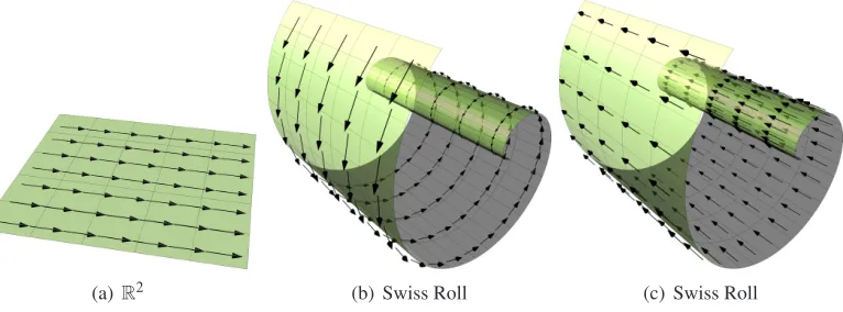
(a)R2 _{(b) Swiss Roll (c) Swiss Roll}

Figure 2: Examples of parallel fields. The parallel fields on Euclidean space are all constant vector fields.

This proposition indicates that finding a local isometryFis equivalent to findingdorthonormal dif-ferentialsd fi,i=1, ...,d, or gradient fields∇fi,i=1, ...,dsince we haveh∇fi,∇fji=hd fi,d fji=

δi j.

3. Parallel Field Embedding

In this section, we introduce our parallel field embedding (PFE) algorithm for dimensionality re-duction.

Our goal is to find a mapF = (f1, . . . ,fd):

M

⊂Rm→Rd which preserves the metric of the manifold. According to Proposition 2, its differential (or gradient fields) should be orthonormal. In the next subsection, we show that if such differential exists, then eachd fi(or∇fi) has to beparallel, that is∇d fi=0 (or∇∇fi=0). Naturally, we propose a vector field based method for solving this problem. We first try to find orthonormal parallel vector fields on the manifold. Then we try to reconstruct the map whose gradient fields can best approximate the parallel fields. In Theorem 2, we show that if the manifold can be isometrically embedded into the Euclidean space, then there exist orthonormal parallel fields and each parallel field is exactly a gradient field. Therefore, in such cases our proposed approach can find the optimal embedding which is a global isometry.

3.1 Parallel Vector Fields

In this subsection, we will show the properties of parallel fields. We will also discuss the relationship among local isometry, global isometry and parallel fields.

Definition 4 (Parallel Field, Petersen, 1998) A vector field X on manifold

M

is a parallel vector field (or parallel field) if

∇X_≡0,

where∇is the covariant derivative on the manifold

M

.

Figure 2 shows some examples of parallel fields on Euclidean space and Swiss Roll. Given a point pon the manifold and a vectorvpon the tangent spaceTp

M

, then∇vpXis a vector at pointpwhich

a vector fieldY, then ∇YX is a vector field which measures how the vector fieldX changes along the vector fieldY on the manifold. Since∇X:Y _7→∇YX is a map which maps a vector fieldY to another vector field∇YX,∇X ≡0 also means that for any vector fieldY on the manifold, we have

∇YX=0 and vice versa. For parallel fields, we also have the following proposition:

Proposition 3 Let V and W be parallel fields on

M

associated with the metric g. We define a

function h:

M

_→R_{as follows:}

h(p) =gp(V,W),

where gprepresents the inner product at p. Then h(p) =constant,∀p∈

M

.

Proof SinceV andWare parallel fields, we have∇V=∇W=0 or∇YV=∇YW=0 for any vector fieldY.

We first show that a vector field is a derivation. For simplicity, let vp be a tangent vector at pointpon Euclidean spaceRm_{. Thenvpdefines the directional derivative in the directionvpatpas}

follows:

vpf =Dvf(p) = d

dt|t=0f(p+tv).

For tangent vectors on a general manifold, we define them as derivations which satisfies the Leib-niz’s rule, that is,vp(f g) = f(p)vpg+g(p)vpf. If p varies, then all thesevps constitute a vector field. Since for each point p, vp is a derivation at p. Then the vector field is a derivation on the manifold. LetX be an arbitrary smooth vector field, then we apply it to the functionhand we have

X(h) = X g(V,W)

= g(∇XV,W) +g(V,∇XW)

= 0+0=0.

The second equation is due to the property of the covariant derivative. Since the above equation holds for arbitraryX, we haveh(p) =gp(V,W) =constant.

Corollary 1 Let V and W be parallel fields on

M

associated with the metric g, thenR_Mg(V,W)dx=

0if and only if_∀p_∈

M

, gp(V,W) =0.

Proof From Proposition 3, we see thatg(V,W) =constant. Thus,R_Mg(V,W)dx=vol(

M

)g(V,W). Since vol(

M

)>0,R_Mg(V,W)dx=0 if and only ifg(V,W) =0 or_∀p_∈

M

,gp(V,W) =0.

This corollary tells us if we want to check the orthogonality of the parallel fields at every point, it suffices to compute the integral of the inner product of the parallel fields. This is much more convenient for finding orthogonal parallel fields.

Also we have the following corollary:

Corollary 2 Let V be a parallel vector field on

M

, then_∀p_∈

M

,_kVp_k=constant where Vp repre-sents the vector at p of the vector field V .

Proof LetW=V in Proposition 3, then_∀p_∈

M

, we have_kVpk2=gp(V,V) =constant.

of the parallel field simply as dividing every tangent vector of the parallel field by a same length. According to these results, finding orthonormal parallel fields becomes much easier: we first find orthogonal parallel fields on the manifold one by one by requiring that the integral of the inner product of two parallel fields is zero. We then normalize the vectors of parallel fields to be unit norm.

Before presenting our main result, we still need to introduce some concepts and properties on the relationship between isometry and parallel fields. We begin with the properties of the differential of a map. We have the following lemma.

Lemma 1 (Please see Lemma 3.5 in Lee, 2003) Let F:

M

_→

N

and let p∈

M

. 1. dF :Tp

M

→TF(p)

N

is linear.

2. If F is a diffeomorphism, then dF :Tp

M

→TF(p)

N

is an isomorphism.

This lemma shows that locallydF is an isomorphism if it is a diffeomorphism. Next, we show that a parallel field is uniquely determined locally.

Proposition 4 Let

M

be an open connected manifold. For a given p_∈

M

, a parallel field X is

uniquely determined by the vector Xp, where Xpdenotes the value of the vector field X on the point

p.

Proof The equation∇X _≡0 is linear inX, so the space of parallel fields is a vector space. There-fore, it suffices to show thatX_≡0 providedXp=0. According to Proposition. 3, a parallel field has constant length. Thus for any pointq_∈

M

, we have_kXqk2=kXpk2=0.

Next we show that the differential of an isometry preserves covariant derivative.

Lemma 2 (Please see the exercise (2) in Chapter 3 of Petersen, 1998) If F:

M

_→

N

is a global isometry, then we have dF(∇XY) =∇dF(X)dF(Y)for all vector fields X and Y .

More importantly, we show that an isometry preserves parallelism, that is, its differential carries a parallel vector field to another parallel vector field.

Proposition 5 If F:

M

_→

N

is a global isometry, then 1. dF maps parallel fields to parallel fields.

2. dF is an isometric isomorphism on the space of parallel fields.

Proof LetY be a parallel field on

M

, we show thatdF(Y)is also a parallel field. It suffices to show that∇ZdF(Y) =0 for arbitraryZ on

N

. According to Lemma 2, for any p_∈

M

and any vector fieldXon

M

, we have∇dF(X)dF(Y) =dF(∇XY) =0 hold at p. SinceX is arbitrary anddF is an isomorphism (Lemma. 1) atp, thendF(X)pcan be an arbitrary vector atp. Since pis also arbitrary, then all these tangent vectorsdF(X)pconstitute an arbitrary vector field. Thus∇ZdF(Y) =0 holds for arbitrary vector fieldZwhich proves the first statement.

local isometry. Combining these two facts,dFis an isometric isomorphism on the space of parallel fields.

Now we show that the gradient fields of a local isometry are also parallel fields.

Proposition 6 If F= (f1, . . . ,fd):

M

_→Rd _{is a local isometry, then each d fi is parallel, that is,}

∇d fi=0, i=1, . . . ,d.

Proof According to the property of local isometry, for very point p_∈

M

, there is a neighborhood U _⊂

M

of psuch that F_|U :U →F(U) is a global isometry ofU onto an open subsetF(U) of

Rd _{(please see Lee, 2003, pg. 187). Since F(U) is an open subset of} Rd_{, we can choose an}

orthonormal basis∂i,i=1, . . . ,d forF(U). SinceF−1|U is also a global isometry, thusdF−1(∂i) is an orthonormal basis ofU. It can be seen as _hdF−1(∂i),dF−1(∂j)i=h∂i,∂ji=δi j. The first equation is due to the definition of isometry. SinceF_|U is a global isometry,dF|U is orthonormal with respect to these coordinates. Thus we can rewriteF_|U asF(x) =Ox+b, wherex∈U,Ois an orthonormal matrix andb_∈Rd_{. Note thatdF= (d f1, . . . ,d fd), thusd fi has constant coefficients}

and we have∇d fi=0 at each local neighborhood. Since we can choose arbitraryp,∇d fi_≡0 holds on the whole manifold.

This proposition tells us that the gradient field of a local isometry is also a parallel field. Since it is usually not easy to find a global isometry directly, in this paper, we try to find a set of orthonormal parallel fields first, and then find an embedding function whose gradient field is equal to the parallel field. Our main theorem will show that such an embedding is a global isometry.

3.2 Objective Function

As stated before, we first try to find vector fields which are as parallel as possible on the manifold. LetV be a smooth vector field on

M

. By definition, the covariant derivative ofV should be zero. That is,∇V _≡0. Naturally, we define our objective function as follows:

E(V) =

Z

Mk

∇V_k2_HSdx, s.t.,

Z

MkVk

2_{=1, (1)}

where_{k · k}HS denotes Hilbert-Schmidt tensor norm (see Defant and Floret, 1993). The constraint removes arbitrary scale of the vector field. Once we obtain the first parallel vector fieldV1, by using orthogonality constraintR_Mg(V1,V2) =0, we can find the second vector fieldV2, and so on. After findingd orthogonal vector fieldsV1, . . . ,Vd, we normalize the vector fields at each point:

kVi_|xk=1,∀x∈

M

, (2)

whereVi|x∈Tx

M

denote the vector atxof the vector fieldVi.

Figure 3: Covariant derivative demonstration. LetV,Y be two vector fields on manifold

M

. Given a point x_∈

M

, let ∇YV_|x denote the tangent vector at x of the vector field ∇YV, we show how to compute the vector∇YV|x. Letγ(t)be a curve on

M

: γ:I →

M

which satisfiesγ(0) =xandγ′(0) =Yx. Then the covariant derivative along the directiondγ_dt(t)_|t=0 can be computed by projecting dV_dt|t=0 to the tangent space Tx

M

at x. In other words,

∇_γ′₍₀₎V|x=Px(dV_dt|t=0), wherePx:v∈Rm→Px(v)∈Tx

M

is the projection matrix. It is not difficult to check that the computation of∇YV_|x is independent to the choice of the curveγ.

In the following we provide some explanation of our objective function. ∇V is the covariant derivative ofV that measures the change of the vector fieldV. If∇V vanishes,V is a parallel vector field which we are looking for. Formally, ∇V is a (1,1)-tensor which maps a vector fieldY to another vector field∇YV and satisfies∇αYV =α∇YV for any functionα. For a fixed pointx∈

M

, let∇V_|x denote the tensor value atxof the tensor field∇V. It is a linear map on the tangent space Tx

M

. We show what∇V|x is when given an orthonormal basis. Let∂1, . . . ,∂d be an orthonormal basis ofTx

M

, then the element of∇V|xwould begx(∇∂iV,∂j)wheregx(·,·)denote the inner product

at pointx. By the definition of Hilbert-Schmidt tensor norm (see Defant and Floret, 1993), we have

k∇V_|xk2HS = d

∑

i=1 d

∑

j=1

(gx(∇∂iV,∂j))

2

=

d

∑

i=1

gx(∇∂iV,∇∂iV). (3)

The second equation uses the fact gx(∇∂iV,∇∂iV) =∑

d

j=1(gx(∇∂iV,∂j))

2_{. It is important to point} out that the Hilbert-Schmidt norm _k∇V_kHS is independent to the choice of the basis of tangent space. Thus our objective functionE(V) is well defined. According to the above equations, the computation of _k∇V_kHS depends on the computation of the norm of covariant derivative ∇∂iV.

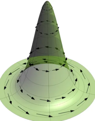
Figure 4: An example of a vector field but not a gradient field. This vector field has loops, thus it cannot be a gradient field for any function.

let ∇YV_|x denote the vector atx of vector field∇YV. Then ∇YV|x is also a vector atx which is demonstrated in Figure 3.

After finding the parallel vector fieldsVi on

M

, the embedding function can be obtained by minimizing the following objective function:

Φ(f) =

Z

Mk∇f−Vk

2_{dx. (4)}

The solution ofΦ(f)is not unique, but differs with a constant function.

In the following, we show that if the manifold is flat and diffeomorphic to an open connected subset of Euclidean spaceRd_{, then our method can successfully recover the metric of the manifold.}

Theorem 2 Let

M

be a d-dimensional Riemannian manifold embedded in Rm_{. If there exist a}

global isometryϕ:

M

_→D_⊂Rd_{, where D is an open connected subset of} Rd_{, then there is an}

orthonormal basis_{Vi}di=1 of the parallel fields on

M

, and embedding function fi:

M

→Rwhose

gradient field satisfies∇fi=Vi,i=1, . . . ,d. Moreover, F= (f1, . . . ,fd)is a global isometry. Proof In Euclidean space, if a vector field is written in Cartesian coordinates, then it is parallel if and only if it has constant coefficients (Petersen, 1998). Consider a parallel field onD. SinceDis open connected, this parallel field is globally constant. Thus the space of parallel fields onDis ad dimensional linear space.

According to Proposition 5, we know that a global isometry preserves parallelism, that is, its differential carries a parallel vector field to another parallel vector field. Thus for a global isometry

also a gradient field. We first mapVi toDusingdϕ. Clearly, dϕ(Vi)is a parallel field. Note that a parallel field in Euclidean space has constant coefficients in Cartesian coordinates. We can write dϕ(Vi)in Cartesian coordinates∂j,j=1, . . . ,das follows:

dϕ(Vi) =

∑

j

c_ij∂j,

wherec_ij are constant. Sincedϕis an isometric isomorphism, we can rewrite it as follows:

Vi=

_∑

j

c_ijdϕ−1_(∂ j).

Heredϕ−1_(∂

j)actually is an orthonormal basis of

M

. Sincecij are constant, eachVi is a gradient field for some linear function with respect to the coordinates ofdϕ−1_(∂

j). Let fibe a linear function such that∇fi=Vi,i=1, . . . ,d. It is worth noting that such a linear function fi is not unique but only differs a constant. Then these_{fi|i=1, . . . ,d}constitutes a mapF,F= (f1, . . . ,fd):

M

→Rd, which maps the manifold

M

toRd_.

Next we show that suchF is a global isometry on

M

. Firstly,F is a local isometry. According to the construction of F, the differential of F dF= (d f1, . . . ,d fd) = (V1, . . . ,Vd) is orthonormal. ThusF is a local isometry according to Proposition 2. Secondly, F is a differmorphism. Clearly the mapF restricted on the manifold

M

,F :

M

_→F(

M

), is surjective. Next we showF is also injective. If not, assume there exist two distinct points pandqsuch thatF(p) =F(q). Then we

have fi(p) = fi(q),i=1, . . . ,d. Since fi is linear with respect to the coordinates ofdϕ−1_(∂

j). We rewrite fi as follows:

fi(p) = d

∑

j=1

c_ijzj(p) +εi,

wherezj,j=1, . . . ,d represent coordinate functions. Sincecij are constant, we havezj(p) =zj(q)

for j=1, . . . ,d. Sincezjare coordinates, we havep=qwhich contradicts to the assumption that p

andqare distinct points. So far, we have provedF is a homeomorphism. Since each fi is a linear function,F is clearly smooth. According to the Proposition 5.7 of Lee (2003),F−1is also smooth, soF is a diffeomorphism. SinceFis a local isometry and a diffeomorphism, it is a global isometry.

When there exists a global isometry, by optimizing our objective functions Equation (1), Equa-tion (2) and EquaEqua-tion (4), Theorem 2 shows that our obtained gradient fields∇fimust be parallel. Moreover, the obtained map F= (f1, . . . ,fd) is a global isometry. It might be worth noting that there are two variations in finding the global isometry. The first variation is the choice of the or-thonormal basis of parallel fields. The second variation is the constant added to each embedding function. Thus the space of global isometry on

M

is actuallyO(d)_×Rd_{. The first part is the space}

of orthonormal basis of parallel fields and the second part is the space of constants. Geometrically, the first part represents a rotation of the map and the second part represents a translation of the map. When there is no isometry between the manifold

M

and Rd_{, our approach can still find a}

when the curvature of the manifold is extremely high, as shown in Figure 4, the obtained vector fields may have loops or singular points and is no longer a gradient field. The resulting embedding may cause overlap. It would be important to note that, in such cases, the isometric embedding or nearly isometric embedding does not exist.

3.3 Implementation

In real problems, the manifold

M

is usually unknown. In this subsection, we discuss how to find the isometric embedding functionFfrom random points.

The implementation includes two steps, first we estimate parallel vector fields on manifold from random points, and then we reconstruct embedding functions by requiring that the gradient fields are as close to the parallel fields as possible. The parallel vector fields are computed one by one under orthogonality constraint. These two steps are described in subsections 3.3.1 and 3.3.2, respectively. After findingd orthonormal vector fields and the corresponding embedding function fi, the final mapFis given byF= (f1, . . . ,fd). We discuss how to perform out-of-sample extension in subsection 3.3.3. The detailed algorithmic procedure is presented in subsection 3.3.4.

Givenxi∈

M

⊂Rm,i=1, ...,n, we aim to find a lower dimensional Euclidean representation of the data such that the geometrical and topological properties can be preserved. We first construct a nearest neighbor graph by eitherε-neighborhood ork nearest neighbors. Letxi_∼xj denote that xi is the neighbor ofxj orxjis the neighbor ofxi. LetN(i)denote the index set of the neighbors of xi, that is,N(i) =

j|xj∼xi . For each pointxi, we estimate its tangent spaceTxi

M

by performing

principal component analysis on the neighborhoodN(i). We choose the largestd eigenvectors as the bases sinceTxi

M

isd dimensional. LetTi ∈R

m×d _{be the matrix whose columns constitute a} orthonormal basis forTxi

M

. It is easy to showPi=TiT

T

i is theuniqueorthogonal projection from

Rm_{onto the tangent spaceTx}

i

M

(Golub and Loan, 1996). That is, for any vectora∈R

m_{, we have} Pia∈Txi

M

and(a−Pia)⊥Pia.

3.3.1 PARALLELVECTORFIELDESTIMATION

LetV be a vector field on manifold. For each pointxi, letVxi denote the value of the vector fieldV

atxi and∇V|xi denote the value of∇V atxi. According to the definition of vector fields,Vxi should

be a tangent vector in the tangent spaceTxi

M

. Thus it can be represented by local coordinates of

the tangent space,

Vxi =Tivi, (5)

wherevi∈Rd. We define V= vT1, . . . ,vTn

T

∈Rdn_{. That is,} V_{is adn-dimensional big column}

vector which concatenates all thevi’s. By discretizing the objective function (1), the parallel fieldV can be obtained by solving the following optimization problem:

min

V E(

V) =

n

∑

i=1

k∇V|xik

2 HS, s.t. _kV_k=1.

(6)

In the following we discuss, for a given pointxi, how to approximatek∇V|xikHS.

vector. Then the covariant derivative of vector fieldV alongei jis given by (please see Figure 3)

∇ei jV = Pi(

dV dt |t=0)

= Pilim

t_→0

V(γ(t))₋V(γ(0))

t

= Pi

(Vxj−Vxi)

di j

≈ √wi j(PiVxj−Vxi),

wheredi j≈1/√wi j approximates the geodesic distancedi j ofxiandxj. There are several ways to define the weightswi j. Since for neighboring points, Euclidean distance is a good approximation to the geodesic distance, we can define the Euclidean weights as wi j = 1

kxi−xjk2. If the data are

uniformly sampled from the manifold, then wi j would be almost constant. So in practice, 0₋1 weights is also widely used which is defined as follows:

wi j =

(

1, ifxi_∼xj 0, otherwise.

Since we do not know ∇∂iV for a given basis ∂i, k∇Vk

2

HS can not be computed according to Equation (3). We define a(0,2)symmetric tensorαasα(X,Y) =g(∇XV,∇YV), whereXandY are vector fields on manifold. We have

Trace(α) =

d

∑

i=1

g(∇∂iV,∇∂iV)

= _k∇V_k2_HS,

where∂1, . . . ,∂d is an orthonormal basis on tangent space. For the trace ofα, we have the following geometric interpretation (see the exercise 1.12 in Chow et al., 2006):

Trace(α) = 1

ωd

Z

Sd−1α(X,X)dδ(X),

whereSd−1is the unit(d₋1)-sphere,dωdis its volume, anddδis its volume form. Thus for a given pointxi, we can approximate_k∇V_|xikHSby the following

k∇V_|xik

2

HS = Trace(α)xi

= 1

ωd

Z

Sd−1α(X,X)|xidδ(X)

≈

∑

j∈N(i)

k∇ei jVk

2

=

_∑

j∈N(i) wi j

P_iV_xj−V_xi

2

. (7)

are uniformly sampled. If the sampling is not uniform, then one should use weighted summation to approximate the integral.

Combining Equation (5), the optimization problem Equation (6) reduces to: min

V E(

V_{) =}

∑

i∼j wi j

P_iT_jv_j−T_iv_i

2

,

s.t._kV_k=1.

We first optimizeE(V_{)to find parallel vector fields on manifold, and then re-normalize the vector}

fields locally.

We will now switch to Lagrangian formulation of the problem. The Lagrangian is as follows:

L

=E(V_)−λ(VTV_−1).

By matrix calculus, we have

∂E(V₎

∂vi

= ₋2

∑

j∈N(i)

wi j(T_iT(PiTjvj−Tivi)−TiTPj(PjTivi−Tjvj))

=2

∑

j∈N(i)

wi j((T_iTTjT_jTTi+Id)vi−2TiTTjvj)

=2

∑

j_∈N(i)

wi j((Qi jQT_{i j}+Id)vi₋2Qi jvj),

whereQi j=T_iTTj. Then we have

∂E(V₎

∂V =2BV,B=



 

B11 _··· B1n

..

. . .. ...

Bn1 _··· Bnn



 ,

whereBis adn_×dnsparse block matrix. If we index eachd_×dblock byBi j, then fori=1, . . . ,n, we have

Bii=

∑

j∈N(i)

wi j(Qi jQTi j+I), (8)

Bi j=

(

−2wi jQi j, ifxi_∼xj

0, otherwise. (9)

Requiring that the gradient of

L

vanish gives the following eigenvector problem:

BV_=λV_.

which can be discretely approximated as_hV_i,V_ji. Since the matrixBis symmetric, its eigenvectors are mutually orthogonal and, thus,_hV_i,V_ji=0.

Recall Corollary 2 tells us for any point p_∈

M

, the tangent vectorVpof a parallel fieldV has a constant length. In our objective function (6), we only need to add a global normalization constraint kV_{k=1 for the sake of simplicity. After finding d vector fieldsVj,j=1, . . . ,d, we can further}

ensure local normalization as follows:

kVj_|xik=1,∀i=1, . . . ,n,j=1, . . . ,d.

3.3.2 EMBEDDING

Once the parallel vector fieldsVi are obtained, the embedding functions fi:

M

→Rcan be con-structed by requiring their gradient fields to be as close toVias possible. Recall that, if the manifold is isometric to Euclidean space, then the vector field computed via Equation (1) is also a gradient field. However, if the manifold is not isometric to Euclidean space,V may not be a gradient field. In this case, we try to find the optimal embedding function f in a least-square sense. This can be achieved by solving the following minimization problem:

Φ(f) =

Z

Mk∇f−Vk

2_dx.

In order to discretize the above objective function, we first discuss the Taylor expansion of f on the manifold.

Let exp_x denote the exponential map atx. The exponential map exp_x :Tx

M

→

M

maps the tangent spaceTx

M

to the manifold

M

. Leta_∈Tx

M

be a tangent vector. Then there is aunique geodesicγasatisfyingγa(0) =xwith initial tangent vectorγ′a(0) =a. The corresponding exponential map is defined by exp_x(ta) =γa(t),t∈[0,1]. Locally, the exponential map is a diffeomorphism.

Note that f_◦exp_x:Tx

M

→Ris a smooth function onTx

M

. Then the following Taylor expan-sion of f holds:

f(exp_x(a))_≈ f(x) +_h∇f(x),a_i, (10)

wherea_∈Tx

M

is a sufficiently small tangent vector. In discrete case, let exp_xi denote the exponen-tial map atxi. Since exp_xi is a diffeomorphism, there exists a tangent vectorai j _∈Txi

M

such that

exp_xi(ai j) =xj. We approximateai j by projecting the vector xj−xi to the tangent space, that is, ai j≈Pi(xj−xi). Therefore, Equation (10) can be rewritten as follows:

f(xj) = f(xi) +h∇f(xi),Pi(xj−xi)i. (11)

Since f is unknown,∇f is also unknown. In the following, we discuss how to compute_k∇f(xi)₋

Vxikdiscretely. We first show that the vector norm can be computed by an integral on a unit sphere,

where the unit sphere can be discretely approximated by a neighborhood.

Letebe a unit vector on tangent spaceTx

M

, then we have (see the exercise 1.12 in Chow et al., 2006)

1

ωd

Z

Sd−1hX,ei

2_{dδ(X) =1,}

Furthermore, we have

kb_k2 =

d

∑

i=1

(bi)2

=

d

∑

i=1

(bi)2 1

ωd

Z

Sd−1hX,∂ii 2_dδ(X)

= 1

ωd

Z

Sd−1hX,bi

2_dδ(X).

From Equation (11), we see that

h∇f(xi),Pi(xj−xi)i= f(xj)−f(xi).

Thus, we have

k∇f(xi)₋Vxik

2

= 1

ωd

Z

Sd−1hX,∇f(xi)−Vxii 2_dδ(X)

≈

∑

j∈N(i)

hei j,∇f(xi)₋Vxii

2

=

_∑

j∈N(i) 1

d_{i j}2hai j,∇f(xi)−Vxii 2

≈

∑

j∈N(i)

wi j_hPi(xj−xi),∇f(xi)−Vxii

2

=

_∑

j∈N(i)

wi j (Pi(xj−xi))TVxi−f(xj) +f(xi)

2

,

whereei jis a unit vector andwi j is the weight, and both of which are the same in Section 3.3.1. In the second equation, the integral is approximated by the discrete summation on nearest neighbors which is the same in Equation (7). In the fourth equation, the vector ai j is approximated by the projection vectorPi(xj−xi). Recall that In Section 3.3.1di j is approximated by √1_{wi j} and we have kai j_k=di j. Next we show these two approximations are coincide as long aswi j=O(_kx 1

j−xik2). Let

us take the Euclidean weightwi j=_kx 1

j−xik2 as an example. We have

lim xj→xi

kPi(xj−xi)k2 kxj−xik2

=lim

θ→0cos(θ) 2_=1, whereθis the angle between vectorPi(xj−xi)and vectorxj−xi.

Letyi=f(xi)andy= (y1, . . . ,yn)T. The objective functionΦ(f)can be discretely approximated

byΦ(y)as follows:

Φ(y) =

_∑

i∼j

wi j (Pi(xj−xi))TVxi−yj+yi

2

.

By setting∂Ψ(y)/∂y=0, we get

−

∑

i∼j

wi jsi j(xj−xi)TPiVxi+

∑

i∼j

wi jsi jsT_{i j}

!

wheresi j is an all-zero vector except thei-th element being₋1 and the j-th element being 1. Let L=∑i_∼jwi jsi jsTi j andc=∑i_∼jwi jsi j(xj−xi)TPiVxi. Then we can rewrite the above linear system as

follows

Ly=c. (12)

Algorithm 1PFE (Parallel Field Embedding) Input: Data sampleX= (x1, . . . ,xn)_∈Rm×n

Output: Y = (y1, . . . ,yn)_∈Rd×n

fori=1 tondo

Compute tangent spacesTxiM

end for

Construct matrixBaccording to Equation (8), Equation (9)

Find the smallestdeigenvaluesλ1, . . . ,λd and the associated eigenvectorsV1, . . . ,VdofB forl=1 tod do

Construct vector fieldVl from local representationsV_l

NormalizeVl(xi)to unit-norm for eachxi end for

Solve linear systemLY =c return Y

It is easy to verify thatLis a graph Laplacian matrix (Chung, 1997) and its rank isn−1. Thus, the solution of Equation (12) is not unique. Ify∗ is an optimal solution,y∗+constant is also an optimal solution. By fixingy1=0 in Equation (12), we get a unique solution ofy. This is consistent with the continuous case. If f is an optimal solution of Equation (4), then f+const is also an optimal solution.

3.3.3 OUT-OF-SAMPLEEXTENSION

Most nonlinear manifold learning algorithms do not have straightforward extension for out-of-sample examples. Some efforts (Bengio et al., 2003) are made to generalize existing nonlinear manifold learning algorithms to novel points. We will show that our PFE algorithm has a natural out-of-sample extension.

Given ntraining pointsx1, . . . ,xn andn′ new pointsxn+1, . . . ,xn+n′. Our task is to estimate the

embedding results of the new points. For each new pointxj, we first find itsknearest points in the whole data set. Then we compute its tangent spaceTxj

M

by performing PCA on its neighborhood.

We choose the largest d eigenvectors as the bases of Txj

M

. Let Tj ∈R

m×d _{be the matrix whose} columns constitute a orthonormal basis forTxj

M

. For each vectorVxj, it can be represented by local

coordinates of the tangent space. That is,Vxj =Tjvj.

Since∂E/∂V_=2BV_{andBis a symmetric matrix, we have}

E(V) =VT_BV_{. (13)}

Let V_{= (}VT_o,VT_{n) = v}T_{1, . . . ,v}T_n,vT_n

+1, . . . ,vn+n′T, where V_o denotes the tangent vectors on the

be written as

E(V_{) =}VT_BV₌VT_o VT_n

Boo Bon

Bno Bnn

V_o V_n

.

Requiring∂E(V_)/∂V_{n=0, we obtain the following linear system:}

BnnVn=−BnoVo.

After solving this linear system, we get the optimalV_{n. Actually, one can compute fnin the same}

way, where fndenotes the function values on new points. We first construct the Laplacian matrix involving all points, including both new and old ones. Then taking derivatives with respect to fn, we obtain the following linear system:

Lnnfn=₋Lnofo,

where fo denotes the function values on old points, andLnnandLno are block matrices which are defined in the same way as Bnn andBno. Note that the procedure described above involves only local computation on each neighborhood of new samples and solving two sparse linear systems. Therefore our out-of-sample extension algorithm is quite efficient.

3.3.4 ALGORITHM

The PFE algorithm consists of three steps, which is summarized in Algorithm 1. 3.4 Related Work and Discussion

In this section, we would like to discuss the relationship between our work and related work which are based on Laplacian, Hessian and connection Laplacian operators.

The approximation of the Laplacian operator using the graph Laplacian Chung (1997) has en-joyed a great success in the last decade. Several theoretical results (Belkin and Niyogi, 2005; Hein et al., 2005) also showed the consistency of the approximation. One of the most important features of the graph Laplacian is that it is coordinate free. That is, the definition of the graph Laplacian does not depend on any special coordinate systems. The Laplacian operator based methods are mo-tivated by the smoothness criterion, that is, the norm of the gradientRMk∇fkshould be small. In

the continuous case, with appropriate boundary conditions we have

Z

Mk∇fk

2₌Z

M f L(f)dx. (14)

Most of previous work focuses on approximating the continuous Laplacian operator. Next we show our method provides a direct way to approximate the integral on the left hand side of Equation (14). First note that

k∇f_k2= 1

ωd

Z

Sd−1hX,bi

2_dδ(X).

From Equation (11), we see that

Therefore we have

k∇f(xi)_k2= 1

ωd

Z

Sd−1hX,∇f(xi)i 2_dδ(X)

≈

∑

j∈N(i)

hei j,∇f(xi)i2

=

_∑

j∈N(i) 1

d_{i j}2hai j,∇f(xi)i 2

≈

∑

j∈N(i)

wi j_hPi(xj−xi),∇f(xi)i2

=

_∑

j∈N(i)

wi j(f(xi)₋f(xj))2.

It can be seen that this result is consistent with traditional graph Laplacian methods.

Our method is also closely related to the approximation of Hessian operator. Note that if we replaceV by ∇f in Equation (1),E(V)becomes Hessian functional (Donoho and Grimes, 2003). It is evident by noticing that Hessf =∇∇f. The estimation of Hessian operator is very difficult and challenging. Previous approaches (Donoho and Grimes, 2003; Kim et al., 2009) first estimate normal coordinates on the tangent space, and then estimate the first order derivative of the function at each point, which turns out to be a matrix pseudo-inversion problem. One major limitation of this is that when the number of nearest neighborskis larger thand+d(d₂+1), wheredis the dimension of the manifold, the estimation will be inaccurate and unstable (Kim et al., 2009). This is contradictory to the asymptotic case, since it is not desirable thatkis bounded by a finite number when the data is sufficiently dense. In contrast, we directly estimate the norm of the second order derivative instead of trying to estimate its coefficients, which turns out to be an integral problem over the nearest neighbors. We only need to do simple matrix multiplications to approximate the integral at each point, but do not have to solve matrix inversion problems. Therefore, asymptotically, we would expect our method to be much more accurate and robust for the approximation of the norm of the second order derivative.

The most related work is the Vector Diffusion Maps (VDM, Singer and Wu, 2011) as we both focus on vector fields rather than embedding functions. VDM is based on the heat kernel for vec-tor fields rather than for functions over the data. It first constructs the heat kernel and orthogonal transformations from the weighted graph. Then VDM defines an embedding of the data via full spectral decomposition of the heat kernel. VDM tries to preserve the newly defined vector diffu-sion distance for the data when doing embedding. Singer and Wu (2011) also provided theoretical analysis that the construction for the kernel essentially defines the discrete type of theconnection

Laplacian operatorand they proved the consistency of such an approximation. We first show that

the objective function of finding parallel vector fields of PFE is the same as VDM. According to the Bochner technique (please see Section 3.2 in Chapter 7 of Petersen, 1998), with appropriate boundary conditions we have _Z

Mk∇Vk

2 HS=

Z

Mh∇

∗_{∇V,Vi, (15)}

where ∇∗_{∇ is the connection Laplacian operator. VDM approximated the connection Laplacian}

similar important features but also differ in several aspects. Firstly, we use the same way to represent vector fields by using local coordinates of tangent spaces. Intuitively, this is the most natural way to represent vector fields as long as the data are embedded in Euclidean space, or in other words the data has features. It would be very interesting to consider the problem of how to represent vector fields on the graph data, that is, the data that do not have features. Secondly, the approximation of the covariant derivative is similar but different. The idea of computing the covariant derivative is to find a way to compute the difference between vectors on different tangent spaces. VDM proposed an intrinsic way to compute covariant derivative using the concept ofparallel transport. They first transported the vectors to the same tangent space using the parallel transport, and then compute the difference of vectors on the tangent space. The way of finding the parallel transport between two points is to compute the orthogonal transformation between two corresponding tangent spaces. It turns out that computing the parallel transport is a singular value decomposition problem for each edge of the nearest neighbor graph. Our approach first computes the directional derivative using the (parallel) transport of vectors on Euclidean space, then projects the directional derivative to the corresponding tangent space. The main computational cost is the projection which is the multiplication of matrices with vectors. In continuous cases, they are two different ways to define the covariant derivative. Thirdly, the discrete type connection Laplacian operators (matrixD−1S₋I in VDM and matrixBin PFE) are different. The difference is that the transformation matrix Oi j in VDM is orthogonal but the transformation matrixQi j in PFE is not. It is because that we use different ways to approximate the covariant derivative. It might be also worth noting that if we use the orthogonal transformation matrix to compute the covariant derivative, the resulted connection Laplacian matrix followed by our discrete approximation methods would be the same as VDM. Overall, VDM uses vector fields to define the vector diffusion distance, while PFE uses vector fields to find the isometry. Although the procedures of computing vector fields are similar, the motivation and objective are different.

4. Experiments

In this section, we evaluate our algorithm on several synthetic manifold examples and two real data sets.

4.1 Topology

In this example, we study the effectiveness of different manifold learning algorithms for isometric embedding. The data set contains 2000 points sampled from a swiss roll with a hole, which is a 2D manifold embedded inR3_{. The swiss roll is a highly nonlinear manifold. Classical linear algorithms}

like PCA cannot preserve the manifold structure. On the other hand, the swiss roll is aflat mani-fold with zero-curvature everywhere and thus can be isometrically embedded inR2_{. We compare}

our algorithm with several state-of-the-art nonlinear dimensionality reduction algorithms: Isomap, Laplacian Eigenmaps (LE), Locally Linear Embedding (LLE), Hessian Eigenmaps (HLLE), and Maximum Variance Unfolding (MVU).

−50−40−30−20−10 0 10 20 30 40 50 −80 −70 −60 −50 −40 −30 −20 −10 0

(a)PFE(R:0.00,Rc:0.00)

−50 −40 −30 −20 −10 0 10 20 30 −30 −20 −10 0 10 20 30

(b)Isomap(R:0.06,Rc:0.05)

−0.04 −0.03 −0.02 −0.01 0 0.010.02 0.03 0.040.05 −0.02 −0.01 0 0.01 0.02 0.03 0.04

(c)LE(R:1.00,Rc:0.39)

−3 −2 −1 0 1 2 3 −2.5 −2 −1.5 −1 −0.5 0 0.5 1 1.5 2

(d)LLE(R:0.84,Rc:0.15)

−0.04 −0.03 −0.02 −0.01 0 0.01 0.02 0.03 0.04 −0.04 −0.03 −0.02 −0.01 0 0.01 0.02 0.03

(e) HLLE(R:1.00,Rc:0.21)

−20 −15 −10 −5 0 5 10 15 −15 −10 −5 0 5 10 15

(f) MVU(R:0.38,Rc:0.11)

−5 0 5 10 0 10 20 −10 −5 0 5 10

(g)V1

−5 0 5 10 0 10 20 −10 −5 0 5 10

(h)V2

Figure 5: Isometric embedding of 2000 points on a Swiss Roll with a hole. The number of nearest neighbors (k) is set to the best among_{4, 5, . . . , 20_}for each algorithm when constructing the neighborhood graph. (a)-(f) show the embedding results of various algorithms. (g)-(h) visualize the two vector fields obtained by our algorithm.

−10 −5 0 5 10 0 10 20 −10 −5 0 5 10 15

The embedding results for all algorithms are shown in Figure 5. Both LE and LLE fail to recover the intrinsic rectangular shape of the original manifold. Isomap performs well at the two ends of the swiss roll but generate a big distorted hole in the middle. This is due to the fact that Isomap can not handle non-convex data. MVU also roughly preserved the overall rectangular shape, but it still generates distortions around the hole. Both HLLE and PFE give very good results. However, it would be important to note that our PFE algorithm generates anisometricembedding while the result of HLLE fail to preserve the scale of the coordinates. In order to measure the faithfulness of the embedding in a quantitative way, we employ the normalizedR-score (Goldberg and Ritov, 2009):

R(X,Y) =1

n n

∑

i=1

G(Xi,Yi)/kHXik2F.

HereG(Xi,Yi)is the (normalized)Procrustes statistic(Sibson, 1978) which measures the distance between two configurations of points (the original dataXiand the embeddedYi). H=I₋1_k11T is the centering matrix. A local isometry preserving embedding is considered faithful and thus would get a lowR-score. We also report a variantRc-score (Goldberg and Ritov, 2009)

Rc(X,Y) =1

n n

∑

i=1

Gc(Xi,Yi)/_kHXi_k2_F,

where Gc(Xi,Yi) allows not only rotation and translation, but also rescaling when measuring the distance between two configurations of points. This score can be used to measure conformal map. Please refer to Goldberg and Ritov (2009) for the details ofR-score andRc-score.

We give the measures ofR-score andRc-score for each algorithm in Figure 5. As can be seen, PFE outperforms all the other algorithms by achieving the minimumR-score andRc-score. For R-score, except for PFE, Isomap and MVU, all the other three algorithms give excessively high value because their normalization significantly change the scale of the original coordinates. These three algorithm also performs worse than MVU, Isomap and especially PFE in terms ofRc-score. 4.2 Noise

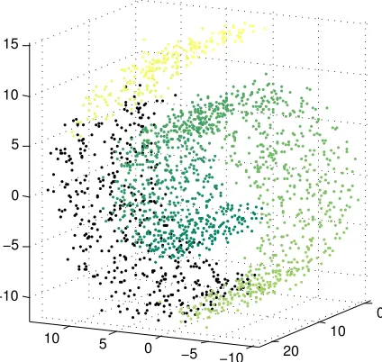
In this example, we compare the performance of different algorithms on noisy data. 2000 points are randomly sampled from the swiss roll without hole, as shown in Fig 6. Then we add random Gaussian noises

N

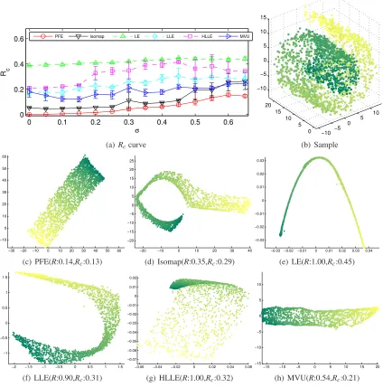
(0,σ2_{)to each dimension. For each givenσ}2_{, we repeat our experiment 10 times} with random noise and the average and standard deviation of theRc-scores are recorded for each algorithm. The results are shown in Figure 7(a). As can be seen, our PFE method consistently outperforms other algorithms and is relatively stable even under heavy noise. Isomap performs the second best. It also achieves very small standard deviation under small noises, but it becomes very unstable whenσ_≥0.5.

Figure 7(b) shows the sample points whenσ=0.65 and Figure 7(c)_∼(h) show the embedding results of different algorithms. As can be seen, under such heavy noise, Isomap, LE, and LLE distort the original Swiss roll. HLLE can expand the manifold correctly to some extent, but there is overlap at the top. MVU unfolds the manifold correctly, but does not preserve the isometry well. Our PFE algorithm can successfully recover the intrinsic structure of the manifold.

0 0.1 0.2 0.3 0.4 0.5 0.6 0 0.2 0.4 0.6 σ R c

PFE Isomap LE LLE HLLE MVU

(a)Rccurve

−10 −5 0 5 10 0 5 10 15 20 −10 −5 0 5 10 15 (b) Sample

−30 −20 −10 0 10 20 30 40 50 60

−10 0 10 20 30 40 50 60

(c) PFE(R:0.14,Rc:0.13)

−20 −10 0 10 20 30 40

−20 −15 −10 −5 0 5 10 15 20 25

(d) Isomap(R:0.35,Rc:0.29)

−0.03−0.02 −0.01 0 0.01 0.02 0.03 0.04

−0.03 −0.02 −0.01 0 0.01 0.02 0.03

(e) LE(R:1.00,Rc:0.45)

−2 −1.5 −1 −0.5 0 0.5 1 1.5

−1 −0.5 0 0.5 1 1.5

(f) LLE(R:0.90,Rc:0.31)

−0.06 −0.04 −0.02 0 0.02 0.04 0.06 −0.07 −0.06 −0.05 −0.04 −0.03 −0.02 −0.01 0 0.01 0.02

(g) HLLE(R:1.00,Rc:0.32)

−15 −10 −5 0 5 10 15 20

−15 −10 −5 0 5 10

(h) MVU(R:0.54,Rc:0.21)

Figure 7: Swiss roll with noise. (a) shows the Rc-scores of the five algorithms. (b) shows the 2000 random points sampled from the swiss roll with noise (σ=0.65). (c_∼h) show the embedding results of the six algorithms.

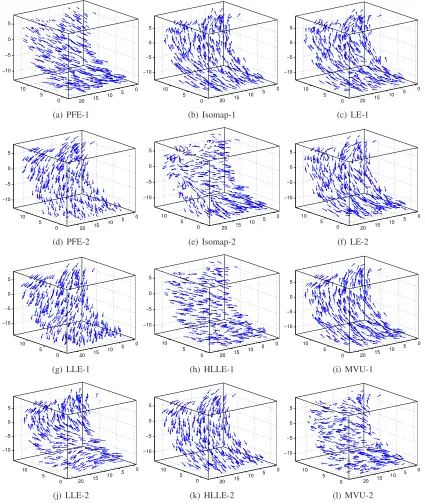
denoted as∇f(xi), by minimizing the following objective function at the local neighborhood ofxi:

∑

j∼i

(f(xj)−f(xi)−(Pi(xj−xi))·∇f(xi))2.

0 5

10 ₅ 0

10 15 20 −10 −5 0 5 (a) PFE-1 0 5

10 ₅ 0

10 15 20 −10 −5 0 5 (b) Isomap-1 0 5

10 ₅ 0

10 15 20 −10 −5 0 5 (c) LE-1 0 5

10 ₅ 0

10 15 20 −10 −5 0 5 (d) PFE-2 0 5

10 ₅ 0

10 15 20 −10 −5 0 5 (e) Isomap-2 0 5

10 ₅ 0

10 15 20 −10 −5 0 5 (f) LE-2 0 5

10 ₅ 0

10 15 20 −10 −5 0 5 (g) LLE-1 0 5

10 ₅ 0

10 15 20 −10 −5 0 5 (h) HLLE-1 0 5 10 0 5 10 15 20 −10 −5 0 5 (i) MVU-1 0 5 10 0 5 10 15 20 −10 −5 0 5 (j) LLE-2 0 5 10 0 5 10 15 20 −10 −5 0 5 (k) HLLE-2 0 5

10 ₅ 0

10 15 20 −10 −5 0 5 (l) MVU-2