Scalable Learning of Bayesian Network Classifiers
Ana M. Mart´ınez [email protected]
Geoffrey I. Webb [email protected]
Faculty of Information Technology Monash University
VIC 3800, Australia
Shenglei Chen tristan [email protected]
College of Information Science/Faculty of Information Technology Nanjing Audit University/Monash University
China/Australia
Nayyar A. Zaidi [email protected]
Faculty of Information Technology Monash University
VIC 3800, Australia
Editor:Russ Greiner
Abstract
Ever increasing data quantity makes ever more urgent the need for highly scalable learners that have good classification performance. Therefore, an out-of-core learner with excellent time and space complexity, along with high expressivity (that is, capacity to learn very complex multivariate probability distributions) is extremely desirable. This paper presents such a learner. We propose an extension to thek-dependence Bayesian classifier (KDB) that discriminatively selects a sub-model of a full KDB classifier. It requires only one additional pass through the training data, making it a three-pass learner. Our extensive experimental evaluation on 16 large data sets reveals that this out-of-core algorithm achieves competitive classification performance, and substantially better training and classification time than state-of-the-art in-core learners such as random forest and linear and non-linear logistic regression.
Keywords: scalable Bayesian classification, feature selection, out-of-core learning, big
data
1. Introduction
Until very recently most machine learning research has been conducted in the context
of relatively small datasets, that is, no more than 50,000 instances and a few hundred
algorithm for very large data should ideally require only a few passes through the training data. Further, to remove memory size as a bottleneck, the algorithm should be able to process data out-of-core.
In this paper, we extend the KDB classifier. KDB is a form of restricted Bayesian network classifier (BNC). It has numerous desirable properties in the context of learning from large quantities of data. These include:
• the capacity to control its bias/variance trade-off with a single parameter,k,
• it does not require data to be held in-core,
• the capacity to learn in just two passes through the training data.
The contributions of this paper are as follows:
• We extend KDB to perform discriminative model selection in a single additional pass
through the training data. In this single pass, our algorithm selects between both attribute subsets and network structures. The resulting highly scalable algorithm combines the computational efficiency of classical generative learning with the low bias of discriminative learning.
• We compare the performance of our algorithm with other state-of-the-art classifiers on
several large datasets, ranging in size from 165 thousand to 54 million instances and 5 to 784 attributes. We show that our highly scalable algorithms achieve comparable or lower error on large data than a range of out-of-core and in-core state-of-the-art classification learning algorithms.
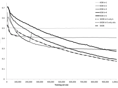
To illustrate our motivations, in Figure 1 we present learning curves for the poker-hand dataset (which is described in Table 7 in Appendix A). As can be seen, for lower quantities
of data the lower variance delivered by low values ofkresults in lower error for KBD, while
for larger quantities of data the lower bias of higher values ofkresults in lower error. While
selective KDB sometimes selects a k that overfits this data with smaller training set sizes,
when the training set size exceeds 550,000 it successfully selects the bestkand by selecting
a subset of the attributes it can substantially reduce error across the entire range of training
set sizes relative to the KDB classifier using the samek.
Section 2 reviews the state-of-the-art in out-of-core BNCs and introduces our proposal: selective KDB (SKDB, Section 2.1). In Section 3 we present a set of comparisons for our
proposed algorithm on 16 big datasets with out-of-core BNCs (Section 3.1), out-of-core
linear classifiers using Stochastic Gradient Descent (Section 3.2), and within-core (batch)
learners BayesNet and Random Forest (Section 3.3). To finalize, Section 4 shows the main conclusions and outlines future work.
2. Scalable Bayesian Networks for Classification
We define the classification learning task as the assignment of a label y ∈ ΩY, from a
set of c labels of the class variable Y, to a given example x = (x1, . . . , xd), with values
for the d attributes A = {X1, . . . , Xd}. Bayesian networks (BN) (Pearl, 1988) provide
0 0.1 0.2 0.3 0.4 0.5 0.6 0.7
0 100,000 200,000 300,000 400,000 500,000 600,000 700,000 800,000 900,000 1,000,000
RMSE
Training set size
KDB k=2 KDB k=3 KDB k=4 KDB k=5 SKDB k=5 only k SKDB k=5 only atts SKDB
Figure 1: Learning curves for KDB and Selective KDB on the poker-hand dataset. The
values plotted are averages over 10 runs. For each run 1,000 examples are se-lected as a test set and samples of successive sizes are sese-lected from the remaining data for training. As can be seen, for lower quantities of data the lower variance delivered by low values ofk results in lower error for KBD, while for larger quan-tities of data the lower bias of higher values of k results in lower error, although there is not sufficient data for k = 5 to asymptote on this dataset. While only selecting a k (SKDB k=5 only k) causes selective KDB to overfit this data with smaller training set sizes (between 20,000 and 550,000), when the training set size is large enough it successfully selects the bestk. Only selecting attributes (SKDB k=5 only atts) always reduces error (relative to KDB k=5). By selecting both k
and attributes (SKDB k=5) selective KDB substantially reduces error relative to KDB with any value ofkonce there are more than approximately 450,000 training examples.
a directed acyclic graph where the the joint probability of all attributes can be written as the product of the individual probabilities of all attributes given their parents, that
is p(y,x) = p(y|πy)Qdi=1p(xi|πxi), where πxi denotes the parents of attribute Xi. If the
structure is known, the likelihood of the BN given the data can be maximized by estimating
p(xi|πxi) using the empirical estimates from the training data T, composed of t training
While unrestricted BNs are the least biased, training such a model on even moderate size data sets can be extremely challenging, as the search-space that needs to be explored grows exponentially with the number of attributes. This has led to restricted BNCs, including naive Bayes (NB) (Duda and Hart, 1973; Minsky, 1961; Lewis, 1998), tree-augmented naive
Bayes (TAN) (Friedman et al., 1997), averaged n-dependence estimators (ANDE) (Webb
et al., 2012) andk-dependence estimators (KDB) (Sahami, 1996). These classifiers have in
common either no structural learning or minimal structural learning that requires only one or two passes through the data. They have been referred to as semi-naive BNCs (Zheng and Webb, 2005). Even though highly biased due to their inherent conditional attribute independence assumption, they have been shown to be very effective classification methods.
NB is the simplest of the BNCs, assuming that all attributes are independent given
the class. It estimates the joint probability using ˆp(y)Qd
i=1pˆ(xi|y), where ˆp(·) denotes an
estimate of p(·). TAN is a structural augmentation of NB where every attribute has as
parents the class and at most one other attribute. The structure is determined by using an extension of the Chow-Liu tree (Chow and Liu, 1968), that utilizes conditional mutual information to find a maximum spanning tree. This alleviates some of NB’s independence assumption and therefore reduces its bias at the expense of increasing its variance. This results in better performance on larger data sets. TAN, provides an intermediate bias-variance trade-off, standing between NB on one hand and unrestricted BNCs on the other.
There has been a lot of prior work that has explored approaches to alleviate NB’s independence assumption. One approach is to add a bounded number of additional in-terdependencies (Friedman et al., 1997; Zheng and Webb, 2000; Webb et al., 2005; Zhang et al., 2005; Yang et al., 2007; Flores et al., 2009a,b; Zheng et al., 2012; Zaidi et al., 2013). At the other extreme, Su and Zhang (2006) propose the use of a full Bayesian network. Of these algorithms, only two approaches allow the number of interdependencies to be ad-justed to best accommodate the best trade-offs between bias and variance for differing data
quantities. ANDE (Webb et al., 2012) averages many BNCs, where a parametern controls
the number of interdependencies to be modeled. KDB uses a parameter k to control the
number of interdependencies modeled.
KDB relaxes NB’s independence assumption by allowing every attribute to be
condi-tioned on the class and, at most, k other attributes. Like TAN, KDB requires two passes
over the training data for learning: the first pass collects the statistics to perform calcula-tions of mutual information for structure learning, and the second performs the parameter learning based on the structure created in the former step (Algorithm 1). An advantage over the ANDE model is that KDB does not need to collect all statistics for all combinations of
nork attributes, allowing it to scale to higher order dependencies. It also has the capacity
to select a model and hence more closely fit the data. This is a disadvantage for small data, which it may overfit, but KDB will often lead to higher accuracy than ANDE on large data which are more difficult to overfit.
Recently, some techniques have been proposed that address the classification problem
with Bayesian networks from a relatively efficient discriminative perspective. Carvalho
Algorithm 1:The KDB algorithm
Input: Training set T with attributes {X1, . . . , Xa, Y}and k.
Output: KDB model.
1 Let G be a directed graphG= (V,E), in whichV is a set of vertices andE is a set of
links.
2 Let Θ be a Bayesian network with structure G.
3 First pass begin
4 G=learnStructure(T) ; /* Algorithm 2 */
5 end
6 Second pass begin
7 Θ = learnParameters(T, G) ; /* Algorithm 3 */
8 end
9 Let KDB be a BN with structure G and conditional probability
distributions in Θ.
10 return KDB
Algorithm 2:learnStructure(T)
Input: Training set T
Output: G, network structure.
1 Calculate M I(Xi;Y) fromT for all attributes.
2 Calculate M I(Xi;Xj|Y) from T for each pair of attributes (i6=j).
3 Let Lbe a list of all Xi in decreasing order of M I(Xi;Y).
4 V ={Y};E =∅;
5 for i= 1→ L.sizedo
6 V=V ∪ Li;
7 E=E ∪(Y,Li);
8 vk=min(i−1, k);
9 while(vk >0) do
10 m= argmaxj{M I(Li;Lj|Y)|1≤j<i∧(Lj,Li)∈ E}/ ;
11 E=E ∪(Lj,Li);
12 vk=vk−1;
13 end
14 end
15 return G
Algorithm 3:learnParameters(T,G)
Input: Training set T and G.
Output: Θ.
1 Initialize Θ to structureG.
2 Compute the CPTs for Θ from T.
algorithm is suited to learning a BNC in a limited number of passes through the training data.
There have also been some important refinements that improve KDB’s performance.
Bouckaert (2006) proposes averaging all possible network structures for a fixed value of k
(including lower orders). Time complexity is significantly reduced by multiplying the sum
of every attribute given all possible parents in the order. Fork= 2 the authors propose a
simplification that identifies one attribute as super parent and consider for every attribute of the class, possibly the super parent and possibly one other lower ordered attribute. The sum of class probabilities is taken as selecting criteria for the superparent. However they agree that this approach is not easy to implement incrementally for large datasets. Rubio and
G´amez (2011) present a variant of KDB that employs a hill-climbing search to incrementally
build a KDB classifier. This approach requires at least one pass through the data for each attribute.
2.1 Selective KDB
The parameterkcontrols KDB’s bias-variance trade-off. Higherkresults in higher variance
and lower bias. Unfortunately there is no apriori means to preselect a value ofk for which
this trade-off will result in the lowest error for a given training set as this is a complex interplay between the data quantity and the complexity and strength of the interactions between the attributes. A further factor that can increase KDB’s error is that attributes that carry no useful information about the class must be treated as if they do, which invariably introduces some noise into the estimates. Discarding these attributes can both reduce error and classification time. Our proposed algorithm, Selective KDB (SKDB), extends KDB
to select between attribute subsets and values ofk in a single additional pass through the
training data.
In the general case, attribute selection is a complex combinatorial task. Fordattributes
there are 2d alternative attribute subsets that could be explored. Many attribute selection
algorithms utilize either forward selection or backwards elimination hill-climbing strategies (Langley and Sage, 1994; Koller and Sahami, 1996). These start with either no attributes or all attributes and then iteratively add or remove one attribute at a time. This requires that all attribute subsets resulting from adding/removing any one attribute are considered
at each step. There are at mostdsuch steps resulting inO(d2) attribute subset evaluations.
If all candidate modifications to a current subset are considered simultaneously in a single
pass through the data, this implies up to dpasses for the attribute selection stage.
We seek to perform both attribute and best-k selection in a single pass. For attribute
selection, we take advantage of the attribute ordering selected by KDB based on mutual information with the class. Given that the attributes are sorted on this order, we consider
only the attribute sets {x1, . . . xi},1 ≤ i≤ d, that is attribute sets that each contain the
i attributes that have the greatest mutual information with the class. These d attribute
subsets are evaluated simultaneously in a single pass through the data using leave-one-out cross validation (LOOCV). For big data, LOOCV can be expected to provide an unbiased
low-variance estimate of the out-of-sample error. It is possible to efficiently evaluate all d
subsets simultaneously, because a KDB classifier using subset{x1, . . . xi}is a minor addition
already incorporates all the calculations for all the KDB classifiers using subsets that we consider.
We use incremental cross validation (Kohavi, 1995), which performs LOOCV on BNCs very efficiently. A naive approach to LOOCV will for each holdout example recalculate from scratch all of the joint frequency counts required by a BNC. Incremental cross-validation first gathers the counts for all training examples in a single pass through the data. Then, when classifying a holdout example, its counts are removed from the table. SKDB collects the complete counts in its second pass through the training data and performs LOOCV in a third pass.
Using the given order, the number of attributes with the best leave-one-out error is selected. In case of a draw, preference is given to the smallest number of attributes. Any
loss function can be used that is a function, {hyx,pˆ(Y,x)i | x ∈ T } → R over all objects
x ∈ T of a predicted class distribution ˆp(Y,x) and the true class for that object, yx.
Such loss functions include 0-1 loss, root mean square error, log-loss, Matthews correlation coefficient (Matthews, 1975) or Brier score (Brier, 1950) to name a few. Because we believe it to be an effective measure of the calibration of a classifier’s class probability estimates, we use root mean squared error (RMSE) as follows:
RM SE = s
1
t
X
x∈T
(1−pˆ(yx|x))2 (1)
where ˆp(yx|x) is the estimated posterior probability of the true class givenx, yx the class
label for the example x.
In order to make full use of available computational resources while reducing the risk of
overfitting, we propose to select algorithmically the best value ofkfor a particular dataset.
Just as the KDB classifiers built on successive attribute subsets are embedded one inside
the other, a KDB classifier withk=i, can be evaluated with little additional computational
effort during the process of evaluating a KDB classifier with k =i+ 1. We leverage this
capacity to simultaneously evaluate KDB classifiers with all attribute subsets{x1, . . . xi−1}
and values of k up to the maximum capacity available, taking advantage of the above
mentioned LOOCV. The combination of attribute subset and k with the best LOOCV
error is selected. In case of a draw, the smaller attribute subset and smaller value of kare
selected. The resulting SKDB algorithm is presented in Algorithm 4.
In the first pass our implementation of SKDB generates a three-dimensional table of co-occurrence counts for each pair of attribute values and each class value. This is required to calculate the mutual information of each attribute with the class and the conditional mutual information of every pair of attributes given the class. The resulting space complexity
is O(c(dv)2). The time complexity of forming the three dimensional probability table is
O(td2), as an entry must be updated for every training case and every combination of two
attribute-values for that case. To calculate the conditional mutual informations, SKDB must consider every pairwise combination of their respective values in conjunction with
each class value O(c(dv)2). Attribute ordering and parent assignment are O(dlogd) and
O(d2logd) respectively.
The second pass requiresdtables ofk+ 2 dimensions (one for each ofkparents, one for
Algorithm 4: The SKDB algorithm
Input: Training set T with attributes {X1, . . . , Xa, Y}and kmax.
Output: SKDB model. 1 First pass begin
2 G=learnStructure(T) ; /* Algorithm 2 */
3 end
4 Second pass begin
5 Θ = learnParameters(T, G) ; /* Algorithm 3 */
6 end
7 Let L be a list of all Xi in decreasing order of M I(Xi;Y). 8 Let P be a kxa matrix of posterior probabilities;
9 Let LF be a matrix of LOOCV results (of length kxa); Initialize it with
zeros;
10 Let Θ↓x be the BN Θ with example x discounted from its CPTs; 11 Third pass (∀x∈ T) begin
12 for k0 = 1 tokmax do
13 P[k0][y∗] = ˆpΘ↓x(y∗|x), ∀y∗ ∈Y;
14 for l= 1→l=L.size do 15 Xmax=L.nextElement;
16 P[k0][y∗] =P[k0][y∗]·pˆΘ↓x(xmax|pak 0
xmax, y
∗), ∀y∗ ∈Ω
Y; where pak 0
xmax are
the k0 first parent-values of Xmax in x.
17 LF[k0][l] =LF[k0][l] +LossF unction(P[k0], yx); where P[k0] is the
vector of posterior probabilities considering the top l attributes by MI.
18 end
19 end
20 end
21 Select b and k indexes with best LF;
22 Truncate Θto attribute subset {1. . . b} and maximum number of parents k; 23 return Θ;
The algorithm to this stage is simply KDB, with time complexity O(td2+c(dv)2+tdk),
wherev is the maximum number of values per attribute, and space complexityO(cdvk+1).
SKDB then extends KDB with an extra pass through the training data to perform
leave-one-out cross validation for the different (ordered) attributesO(tcdk).
At classification time, SKDB need only store the conditional probability distribution for
thedb selected attributes and thekb selected,O(cdbvbk). The time complexity of classifying
a single example is O(cdbkb).
In summary, SKDB requires an extra pass over the data compared with KDB, and the complexity of this extra pass is linearly dependent on the number of training examples,
classes, attributes andkso the order of the time complexity increases fromO(td2+c(dv)2+
tdk) toO(td2+c(dv)2+tcdk). This is not a great increase in practice, since the number of
pass can dominate that of the subsequent passes. Classification time and space complexity
are reduced compared to KDB if the number of selected attributesdb< dand/orkb< kmax.
For the cost of this modest increase in computation, KDB is extended so as to discrim-inatively choose between a large class of alternative BNC models. Note that while it is possible to use cross validation to select between any collection of alternative models, it is only possible to do so in the extremely efficient manner we have developed for a very restricted class of learners, those that can be evaluated using incremental cross-validation and can be decomposed into nested models. The only types of learners of which we are aware that belong to this class are KDB and ANDE. We leave applying the approach to ANDE and variants of KDB as a topic for future research.
It may be possible to gain further efficiencies through sampling. As discussed in Hulten and Domingos (2002), it is sometimes possible to obtain sufficiently accurate estimates of the parameters for a learning program from a subsample of the full data. For very large datasets we could potentially utilize a random sample for the first pass of our algorithm, which only needs to estimate the parameters for three-way interactions between each pair
of attributes and the class. We believe that the best value of k will usually be the one for
which there is only just enough data in the dataset to obtain sufficiently accurate estimates of the required parameters. Thus we do not believe that sampling will usually be useful for the second pass. A technique such as Racing (Maron and Moore, 1994) could be used to select the model in the final pass. However, we suspect that it will usually require extremely large samples to confidently distinguish between the large number of very similar models that are assessed in the third pass. Given that the computational overheads of scanning a large dataset in random order are considerable, we do not believe that sampling will often be useful. However, this also remains a potential direction for future research.
3. Experimental Methodology
We undertook an extensive online search to gather a group of large datasets, all of which have more than 100K instances. These datasets are described in Table 7 in Appendix A, in ascending order of number of samples. Those below the double line have more than 1
million instances. All datasets except for poker-hand,uscensus1990 and splice contain
one or more numeric attributes. 7 datasets contain only numeric attributes: MITFaceSetA,
MITFaceSetB, MITFaceSetC, Mnist, USPSExtended, MSDYearPrediction and satellite. For the Bayesian network classifiers we discretize numeric attributes using 5-bin equal fre-quency discretization. To avoid loading the whole data into memory, only a random sample of 100K points is used to define the bins for discretization.
As described in Section 2.1, we use SKBD with RMSE as the objective function for the third pass that selects between structures because we believe it to be a good measure of the calibration of a classifier’s class probability predictions. However, this raises the issue that we might be reporting the measure that best favors our approach. To guard against this, we also present in the Appendices 0-1 loss results of the relative performance of all algorithms, and discuss these results in the appropriate sections below. Table 9 shows that when evaluated on RMSE, SKDB trained to optimize RMSE and SKDB trained to optimize
0-1 loss (SKDB0-1) attain identical 0-1 loss on 12 out of 16 datasets, suggesting that SKDB’s
Train Test
time space time space
NB O(td) O(cdv) O(cd) O(cdv)
TAN O(td2+c(dv)2+d2loga) O(c(dv)2) O(cd) O(cdv2)
AODE O(td2) O(c(dv)2) O(cd2) O(c(dv)2)
KDB O(td2+c(dv)2+tdk) O(c(dv)2+cdvk+1) O(cdk) O(cdvk+1)
SKDBk O(td2+c(dv)2+tcdk) O(c(dv)2+cdvk+1) O(cdbk) O(cdbvk+1)
SKDB O(td2+c(dv)2+tcdk) O(c(dv)2+cdvk+1) O(cdbkb) O(cdbvkb+1)
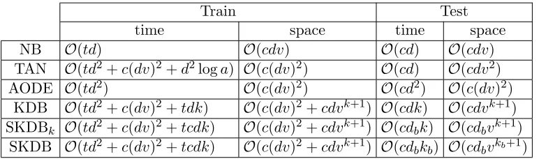
Table 1: Orders of complexity for the different semi-naive BNCs where: t is the number
of training examples, d is the number of attributes, v is the maximum number
of values per attribute, c the number of classes, db (the best d) is the remaining
attributes after applying SKDB, and kb (the best k) is the k value selected in
SKDB.
The structure of the experimental Section is as follows: Section 3.1 compares our pro-posed SKDB algorithm’s results with different out-of-core semi-naive BNCs. Section 3.2
compares our SKDB algorithm with several online (out-of-core) linear classifiers. Section
3.3 includes comparisons with two state-of-the-art in-core machine learning algorithms, BayesNet (Augmented Bayesian network) and Random Forest. Section 3.4 presents a global comparison of all learners considered, along with empirical time comparisons for the differ-ent out-of-core classifiers. Each of these sections provides a summary of the relevant results. Detailed RMSE error outcomes are presented in Table 8 in Appendix A and a more detailed analysis of results is provided in in Appendix C.
All the experiments for the Bayesian out-of-core algorithms use C++ software specially
designed to deal with out-of-core classification methods1. Appendix B specifies the
imple-mentation details.
Note that both RMSE and 0-1 Loss are assessed using 10-fold cross-validation. This should not be confused with the leave-one-out cross-validation used to select the number of attributes and parents in SKDB. For each fold of the 10-fold cross-validation, SKDB performs leave-one-out cross-validation on the training set to select the parameters of the model that is then tested on the holdout test fold.
3.1 SKDB vs Bayesian Out-of-core Algorithms
The first set of experiments compare SKDB with the out-of-core semi-naive BNCs described in Section 2: NB, TAN, AODE and KDB. We also consider a version of SKDB which fixes
the value ofk and just selects among the attributes, referred to as SKDBk. Table 1 shows
a summary of the orders of complexity for all these BNCs.
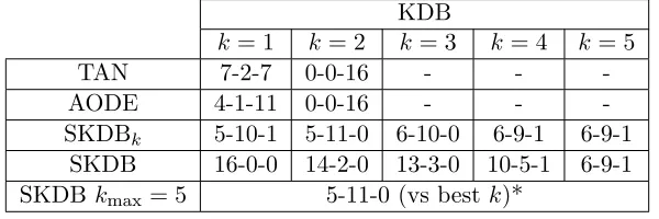
Tables 2 and 3 show win-draw-loss records summarizing the relative RMSE and 0-1 loss
of the different approaches. Cell [i, j] of each table contains the number of wins/draw/losses
KDB
k= 1 k= 2 k= 3 k= 4 k= 5
TAN 6-3-7 0-0-16 - -
-AODE 3-0-13 0-0-16 - -
-SKDBk 8-8-0 6-10-0 6-10-0 7-9-0 6-9-1
SKDB 16-0-0 16-0-0 14-2-0 14-2-0 8-8-0
SKDBkmax= 5 6-10-0 (vs bestk)*
* The result is 6-9-1 (shift in uscensus) if SKDB is optimized with 0-1 loss.
Table 2: Win-draw-loss records when comparing the RMSE of different out-of-core BNCs.
KDB
k= 1 k= 2 k= 3 k= 4 k= 5
TAN 7-2-7 0-0-16 - -
-AODE 4-1-11 0-0-16 - -
-SKDBk 5-10-1 5-11-0 6-10-0 6-9-1 6-9-1
SKDB 16-0-0 14-2-0 13-3-0 10-5-1 6-9-1
SKDBkmax= 5 5-11-0 (vs bestk)*
* The result is 6-10-0 if SKDB is optimized with 0-1 loss.
Table 3: Win-draw-loss records when comparing the 0-1 loss of different out-of-core BNCs.
for the classifier on row iagainst the classifier on columnj. A win indicates that the
algo-rithm has significantly lower error than the comparator. A draw indicates that the differ-ences in error are not significant. Statistical significance has been assessed using Wilcoxon
signed-rank tests to compare the 10-fold outputs. SKDBk and SKDB are compared against
standard KDB with the same value of k. Additionally, SKDB with k = 5 is compared
against the lowest error of any standard KDB withkbetween 1 and 5 (which is a
theoreti-cal result, since the value ofkthat will minimize out of sample error can only be determined
a posteriori).
The results indicate that TAN is competitive with KDB k = 1, whereas AODE only
achieves lower error on three or four of the datasets, depending on the loss function. We believe the reason AODE performs so poorly is that the advantage it gets in reduced
vari-ance from ensembling the d models is less useful for larger data. Both TAN and AODE
consistently show higher error than higher orders of KDB on these large datasets. SKDBk
only increases the RMSE of KDB relative to one value of kand only on one dataset,
MIT-FaceSetB, and then only from 0.0841 to 0.0844. For many datasets it does not affect error
(but nonetheless speeds up classification time). For many datasets it substantially reduces
error, such as the reduction from 0.2048 to 0.1868 for poker-hand.
The average bestkfor SKDB across the 16 datasets is 4.08. On average, 78.46±29% of
0.01 0.1 1 0.01
0.1 1
MITFaceSetA MITFaceSetB MITFaceSetC
MSDYearPrediction
USPSExtended PAMAP2
Census-income covtype
linkage
kddcup
localization
mnist8ms poker-hand
satellite
splice uscensus
KDB (k=5) - RMSE (log. scale)
S
K
D
B
(
m
ax
k
=
5)
R
M
S
E
(
lo
g.
s
ca
le
)
(a) KDB withk= 5 and SKDB (kmax= 5).
0.01 0.1 1
0.01 0.1 1
MITFaceSetA
MITFaceSetB MITFaceSetC
MSDYearPrediction
USPSExtended PAMAP2
Census-income covtype
linkage
kddcup
localization
mnist8ms poker-hand
satellite
splice uscensus
KDB (best k) - RMSE (log. scale)
S
K
D
B
(
m
ax
k
=
5)
R
M
S
E
(
lo
g.
s
ca
le
)
(b) KDB with the bestkfor each dataset and SKDB (kmax= 5).
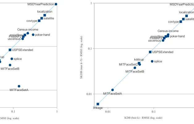
Figure 2: Scatter plot of RMSE comparisons for KDB and SKDB.
obtains the same results as KDB with the best value of k, but reducing the number of
attributes. Indeed, reducing the number of attributes without affecting error is the worst case encountered by SKDB, because it never loses in terms of RMSE compared to the best KDB).
One could think that KDB with k = 5 would be the fairest comparison with SKDB
(kmax= 5). This comparison is shown in Figure 2a, where the X-axis represents the RMSE
results with KDB with k = 5 for the 16 datasets and the Y-axis the RMSE with SKDB.
We have used a logarithmic scale because almost half of the points fall below the 0.1 range.
Note that there is not a single point above the diagonal line, which indicates that SKDB is
never worse than KDB k = 5 or even KDB with the best k value considered, as shown in
Figure 2b.
If only the best number of parents is selected by SKDB (bestk) and no feature selection
is performed, then the RMSE is always equivalent to the best RMSE obtained by KDB
with any value of k ∈ {1,5}. That is, for all datasets SKDB without attribute selection
is successful at selecting the best value of k with respect to the specified loss function.
However, for five datasets the value of k that attains the best RMSE is different to that
which attains the best 0-1 loss, demonstrating the value of optimizing with respect to the
relevant loss function. These results are summarized on row SKDBonlyk in Tables 8 and 9.
Learner
T
ime (seconds)
KDB1 SKDB1 KDB5 SKDB5
0
500
1000
2000
(a) Training Times
Learner
T
ime (seconds)
KDB1 SKDB1 KDB5 SKDB5
0
10
20
30
40
50
60
(b) Classification Times
Figure 3: Training and classification time comparisons for KDB and SKDBk.
complex evaluation functions were to be used in a highly time-constrained scenario, then only a random sample of instances could be considered at this step.
Figures 3a and 3b show the training and classification time comparisons for KDB and
SKDBk. Only the 11 smallest out of the 16 datasets have been considered for time
mea-surement, since these experiments have been conducted on a desktop computer with an Intel(R) Core(TM) i5-2400 CPU @ 3.10 GHz, 3101 MHz, 64 bits and 7866 MiB of memory, whereas the remaining experiments have been conducted in a heterogeneous grid environ-ment for which CPU times are not commensurable. Each bar represents the sum of all 11
datasets2 in a 10-fold cross validation experiment. These graphs reinforce what the orders
of complexity for the two algorithms indicated, that is, SKDBkrequires a bit more time for
training (extra pass on the data), while the classification time is less in practice, since the
number of attributes selected is generally smaller than d.
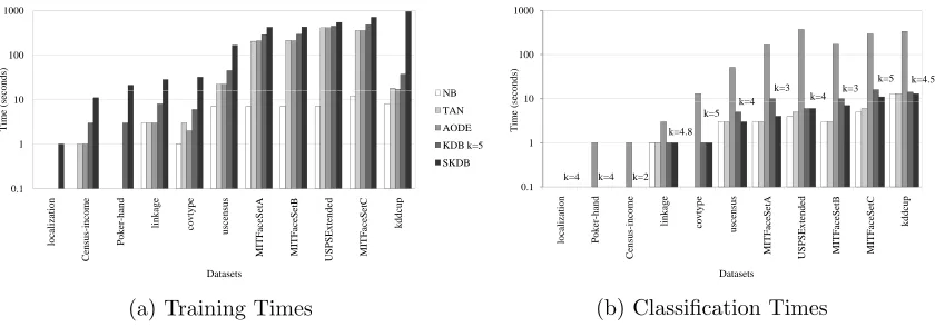
Figures 4a and 4b show the training and classification empirical time comparisons of the
different out-of-core BNCs relative to SKDB (with kmax=5). The datasets are ordered at
increasing time for SKDB. Note that SKDB always takes a bit more time for training, taking
the largest time forkddcup, due to its large number of classes. Nevertheless, for the datasets
with many attributes: MITFaceSetA, MITFaceSetB, USPSExtended and MITFaceSetC; the
time differences with other BNCs become smaller. At classification time some gain can be
appreciated for SKDB compared to KDB k = 5 if the selected k is less than 5. AODE’s
classification time is quadratic in the number of attributes, and hence much higher for all datasets.
3.2 SKDB vs Non-Bayesian Out-of-core Algorithms
In this section we compare SKDB with the state-of-the-art in online learning: Logistic Re-gression with Stochastic Gradient Descent (LRSGD). We use LRSGD’s implementation in Vowpal Wabbit (VW) (Agarwal et al., 2014), an open source out-of-core linear learning sys-tem. VW provides a scalable implementation of LRSGD, which can be used in combination with several loss functions, different parameters for the learning rate and regularization, and quadratic or cubic combination of features.
100 1000
on
ds)
NB
0 1 1 10
Tim
e (sec
NB TAN AODE KDB k=5 SKDB
0.1
localization
Censu
s-i
ncom
e
Poker-han
d
li
nkag
e
covt
y
p
e
uscensus
MITFaceSetA MITFaceSetB USPSE
xt
ended
MITFaceSetC
kddcup
Datasets
(a) Training Times
k=4 k=3
k=4 k=3
k=5 k=4.5
10 100 1000
se
conds)
k=4 k=4 k=2
k=4.8 k=5
k=4
0.1 1 10
n d
m
e ge
p
e us A d B C p
Tim
e (
s
loc
aliza
tio
n
P
o
ke
r-ha
n
C
ens
us-inc
o
m
linka
g
covty
p
us
ce
ns
u
MI
TFa
ceSe
tA
USPSE
x
tende
MI
TFace
Set
B
MI
TFace
Set
C
kd
dcu
p
Datasets
(b) Classification Times
Figure 4: Time comparisons per dataset for NB, TAN, AODE, KDB against SKDB.
We have performed experiments with varying numbers of passes for LRSGD, varying loss functions and combinations of features. We use the default advanced (step size) updates provided by VW, which are:
1. Importance weight invariance (Karampatziakis and Langford, 2011): this update is meant to be useful specially for cost-sensitive learning, that is, when the misclassi-fication penalty varies for the different class labels. However, it is also claimed to reduce classification error even when no matrix of weights is provided. The following equation is used to compute the weights:
wi←wi−s(ηI)
∂L(ˆyw(x), y)
∂wi
, (2)
where y is the true class; ˆyw(x) is the predicted value for example x ∈ Rd with
parameters w∈Rd; L(ˆyw(x), y) is the loss function; η is the learning rate;I ∈Nthe
number of times an example is more important than a typical example, in our case
I = 1; ands(ηI) is a scaling factor, for which a closed form solution can be found for
each loss function (Karampatziakis and Langford, 2011) .
2. Adaptive updates (Duchi et al., 2011; McMahan and Streeter, 2010): the learning
rate must decay to converge. Instead of usingηt= √1t orηt = 1t at iteration t for all
features, we use a per-feature learning rate decay:
wi ←wi−η
git q
Pt
t0=1git20
, git=
∂L(ˆyw(xt), yt)
∂wi
, (3)
3. Normalized updates (Ross et al., 2013): instead of using Gaussian sphering standard solution, which would imply in-core processing and an increase in the size of the
dataset, a scale-free update is used that renormalizes wi at each timestep and keeps
track of a global scale.
A fair comparison of LRSGD with SKDB should perform the same number of passes
VWLF VWSF
SKDB RMSE 7
(+2)-0-7 14-0-2
0-1 Loss 8(+1)-1-5(+1) 8-1-7
Table 4: Win-draw-loss records for VW and SKDB in terms of RMSE and 0-1 Loss
actually results in n+ 1 passes through the data. This is also true for SKDB on numeric
data, as an extra pass is required for discretization. We have run experiments with 3, 10 and 20 passes for LRSGD. Each 10-fold cross validation experiment is repeated 10 times. Both the quadratic and logistic loss functions are considered. The one-against-all reduction from multiclass classification to binary classification has been used for the datasets with multiple class labels, which creates one binary problem for each of the classes. Table 10 in Appendix A shows the results for all of the different combinations for which we have conducted comprehensive experiments. The overall best results for LRSGD are obtained with 3 passes and using quadratic features. When the squared loss function is optimized we refer to it as VWSF, and VWLF if the logistic function is used. In all cases, SKDB is highly competitive compared to VW.
Note that while LRSGD has a number of parameters that could potentially be tuned using cross validation, doing so does not make a reasonable comparator to SKBD as such tuning would require multiple passes through the data for each cross-validation fold.
A win-draw-loss record summary is displayed on Table 4. The (+1) and (+2) for SKDB
vs VWLF aim at distinguishing the results for satellite and splice, for which more
than 400 hours are required to get the 10cv results using VWLF, and hence VWSF is considered instead. Irrespective of the fact that the SKDB model is optimized with respect to RMSE, the win-draw-loss records only vary for three datasets between evaluation with respect to RMSE or 0-1 loss. The win-draw-loss records remain exactly the same whichever loss function is optimized in VW (see Table 10 for more details).
Since the output of the VW algorithms is not probabilistic, we are using the class prediction, and hence computing 0-1 loss for comparisons with SKDB as well. By using, for
example, the following sigmoid function 1+e−1ywˆ (x), probability estimates can be estimated
from VW. Using this approach, the RMSE results for VWSF are only better than SKDB for two of the datasets (MSDYearPrediction and USPSExtended), both of them originally sparse and containing exclusively numeric attributes. These records improve when using a logistic function for optimization, that is VWLF (see Table 10 in Appendix A for more details). Nevertheless, computation time for VWLF is much larger than for VWSF as shown below.
0.01 0.1 1 0.01
0.1 1
MITFaceSetA MITFaceSetB MITFaceSetC
MSDYearPrediction
USPSExtended
PAMAP2 Census-income
covtype
linkage
kddcup
localization
mnist8ms poker-hand satellite
splice uscensus
VWLF - RMSE (log. scale)
S
K
D
B
(
m
ax
k
=
5)
R
M
S
E
(
lo
g.
s
ca
le
)
(a) RMSE for VWLF and SKDB.
0.01 0.1 1
0.01 0.1 1
MITFaceSetA MITFaceSetB MITFaceSetC
MSDYearPrediction
USPSExtended
PAMAP2 Census-income
covtype
linkage
kddcup localization
mnist8ms poker-hand satellite
splice uscensus
VWSF - RMSE (log. scale)
S
K
D
B
(
m
ax
k
=
5)
R
M
S
E
(
lo
g.
s
ca
le
)
(b) RMSE for VWSF and SKDB.
0.0001 0.001 0.01 0.1 1
0.0001 0.001 0.01 0.1 1
MITFaceSetA MITFaceSetB MITFaceSetC
MSDYearPrediction
USPSExtended
PAMAP2 Census-income
covtype
linkage
kddcup
localization
mnist8ms poker-hand
satellite
splice uscensus
VWLF - 0-1 Loss (log. scale)
S
K
D
B
(
m
ax
k
=
5)
0
-1
L
os
s
(l
og
. s
ca
le
)
(c) 0-1 loss for VWLF and SKDB.
0.0001 0.001 0.01 0.1 1
0.0001 0.001 0.01 0.1 1
MITFaceSetA MITFaceSetB MITFaceSetC
MSDYearPrediction
USPSExtended
PAMAP2 Census-income
covtype
linkage
kddcup
localization
mnist8ms poker-hand
satellite
splice uscensus
VWSF - 0-1 Loss (log. scale)
S
K
D
B
(
m
ax
k
=
5)
0
-1
L
os
s
(l
og
. s
ca
le
)
(d) 0-1 loss for VWSF and SKDB.
Figure 5: Scatter plot of RMSE and 0-1 loss comparisons for VW and SKDB (kmax= 5).
the comparisons of VW with SKDB in terms of 0-1 Loss. In this case, VWSF performs slightly better than VWLF compared to SKDB.
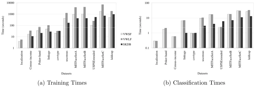
Figure 5 shows the relative training and test times for VW and SKDB across all datasets. SKDB has substantially lower training and test time on most datasets. One exception is the sparse numeric USPSExtended dataset. Another is covtype, which has a large number of sparse boolean attributes.
100 1000 10000
(s
ec
on
ds)
1 10
tion ome and ag
e
y
pe
n
su
s
etA etB ded etC cup
Tím
e
VWSF VWLF SKDB
local
iza
t
C
ensu
s-inc
o
P
oke
r-h
a
li
n
k
covt
y
us
ce
n
MITF
aceS
e
MITFaceS USPSEx
ten
d
MITFaceS
kd
d
c
Datasets (a) Training Times
10 100
(seco
nd
s)
0.1 1
tion and ome age ype nsu
s
etA ded etB etC cup
Ti
m
e
VWSF VWLF SKDB
localiza
t
P
o
ker-h
a
Census-i
n
co
li
nk
covt
y
usce
n
MITFaceS
e
USPSExt
en
d
MITFaceS MITFaceS
kd
d
c
Datasets
(b) Classification Times
Figure 6: Time comparisons per dataset for VW with squared and logistic functions against SKDB.
SKDB takes more than the alternatives, which is USPSExtended. We believe that for this
dataset VW is able to exploit the sparseness of the data while SKDB cannot. Some of the reasons why VW is taking in general more time than SKDB both for training and classifying is the consideration of quadratic features, the need to binarize discrete attributes (creating many binary attributes) and the need also to use one-against-all for multiclass classification.
3.3 SKDB vs In-core Algorithms
In order to understand how much predictive capacity, if any, is sacrificed by using our out-of-core classifiers, it is useful to compare them to the state-of-the-art in in-core classification. To this end, we have replicated our set of experiments with two in-core algorithms: a more general BNC and Random Forest, a powerful exemplar of the state-of-the-art. For some datasets it was infeasible to get results, even with high-performance computers, due either
to time or memory limitations (indicated in Table 8 in Appendix A with > 600h, when
more than 600 CPU hours are required; or by >138G, when more than 138GB of RAM
memory are required).
Note that while each of these algorithms has a number of parameters that could po-tentially be tuned using cross validation, doing so would not make reasonable comparators to SKBD. First, SKDB uses cross-validation to choose between multiple models rather than to choose between parameterizations. Cross validation could also be used to tune SKBD parameters such as the smoothing technique. Second, SKDB uses cross-validation in a constrained manner that requires only a single additional pass through the data while parameter tuning of these algorithms would increase compute time proportionally to the number of folds employed.
3.3.1 Augmented Bayesian Network
BayesNet
SKDB 6(+4)-3-3
Table 5: Win-draw-loss records for BayesNet and SKDB in terms of RMSE.
deletion, that is, arcs from the class to the attributes can be removed). It optimizes the K2 metric (Cooper and Herskovits, 1992). The maximum number of parents allowed for a node in the Bayes net is set to 5. The win-draw-loss comparison is presented in Table 5.
The detailed results can be found in Table 8 (Appendix A), row BayesNet. The
darker grey background corresponds to those cases where BayesNet significantly outper-forms SKDB. Note that there are only records for 12 out of the 16 datasets, because there are four cases for which results could not be computed for BayesNet due to memory con-straints, since the network cannot be learned incrementally.
Even though BayesNet performs a more exhaustive search than SKDB of the model space of Bayesian networks with up to 5 parents, SKDB obtains lower error than BayesNet more often than the reverse. We hypothesize that this is due to SKDB’s use of both generative and discriminative measures for model selection in contrast to BayesNet’s use exclusively of generative measures.
3.3.2 Random Forest
Random Forest (RF) is a state-of-the-art learning algorithm introduced in Breiman (2001). It uses bagging (Breiman, 1996) to aggregate an ensemble of trees that are each grown using a process that involves a stochastic element to increase diversity.
We have conducted experiments with RF selecting 100 trees. We present results both with pre-discretized data, to show relative performance on categorical data, and with undis-cretized data. The detailed results can be found on the fifth and sixth from last rows in Table 8 in Appendix A. Table 6 shows the win-draw-loss records when compared with SKDB. The superscripts compute those datasets for which results cannot be obtained for
RF due to main memory constrains (>138G are required). The results show that SKDB
is competitive with RF in terms of RMSE, even when RF is performing its own discretiza-tion (5 wins for SKDB and 6 wins for RF), for which the computadiscretiza-tional cost in terms of memory and time is much higher than SKDB’s. When 0-1 Loss is considered, out-of-core RF wins more frequently than SKDB, even when 0-1 Loss is used as the objective function during structure selection. When MDL discretization is used instead of 5EF for SKDB, then the results improve slightly for SKDB compared to RF performing its own discretization. When interpreting these results it is important to keep in mind that SKDB is a 3-pass out-of-core algorithm (4-pass with discretization) in contrast to the inherently computationally intensive in-core processing of RF.
Note that the sum of some cells is not exactly 16 but smaller, due to computational constraints for RF. RF is an in-core algorithm, and hence we have not been able to learn classification models for the largest datasets. Interestingly, RF is more negatively affected (in terms of computation) by a large number of classes than the BNCs, for example no 100
tree model can be learnt forMSDYearPrediction, which has 90 class labels. Precisely, there
RF (5EF) RF (Num)
RMSE SKDB 5(+4)-1-6 5(+5)-0-6
0-1 Loss
SKDB 2(+4)-3-7 2(+5)-2-7
SKDB0−1 3(+4)-2-7 3(+5)-1-7
SKDBM DL 8(+4)-2-2 3(+5)-2-6
Table 6: Win-draw-loss records for RF and SKDB in terms of RMSE and 0-1 Loss.
0.01 0.1 1
0.01 0.1 1
MITFaceSetA
MITFaceSetBMITFaceSetC
MSDYearPrediction
USPSExtended PAMAP2
Census-income covtype
linkage
kddcup
localization
mnist8ms poker-hand satellite
splice uscensus
BayesNet - RMSE (log. scale)
S
K
D
B
(
m
ax
k
=
5)
R
M
S
E
(
lo
g.
s
ca
le
)
0.01 0.1 1
0.01 0.1 1
MITFaceSetA MITFaceSetB
MITFaceSetC
MSDYearPrediction
USPSExtended PAMAP2
Census-income covtype
linkage
kddcup
localization
mnist8ms poker-hand
satellite
splice
uscensus
RF - RMSE (log. scale)
S
K
D
B
(
m
ax
k
=
5)
R
M
S
E
(
lo
g.
s
ca
le
)
(a) BayesNet and SKDB.
0.01 0.1 1
0.01 0.1 1
MITFaceSetA
MITFaceSetBMITFaceSetC
MSDYearPrediction
USPSExtended PAMAP2
Census-income covtype
linkage
kddcup
localization
mnist8ms poker-hand satellite
splice uscensus
BayesNet - RMSE (log. scale)
S
K
D
B
(
m
ax
k
=
5)
R
M
S
E
(
lo
g.
s
ca
le
)
0.01 0.1 1
0.01 0.1 1
MITFaceSetA MITFaceSetB
MITFaceSetC
MSDYearPrediction
USPSExtended PAMAP2
Census-income covtype
linkage
kddcup
localization
mnist8ms poker-hand
satellite
splice
uscensus
RF - RMSE (log. scale)
S
K
D
B
(
m
ax
k
=
5)
R
M
S
E
(
lo
g.
s
ca
le
)
(b) RF and SKDB.
Figure 7: Scatter plot of RMSE comparisons for BayesNet, RF and SKDB.
trees. These four datasets are MSDYearPrediction,satellite, mnist8msand splice, so
the largest possible samples able to be computed have been considered.
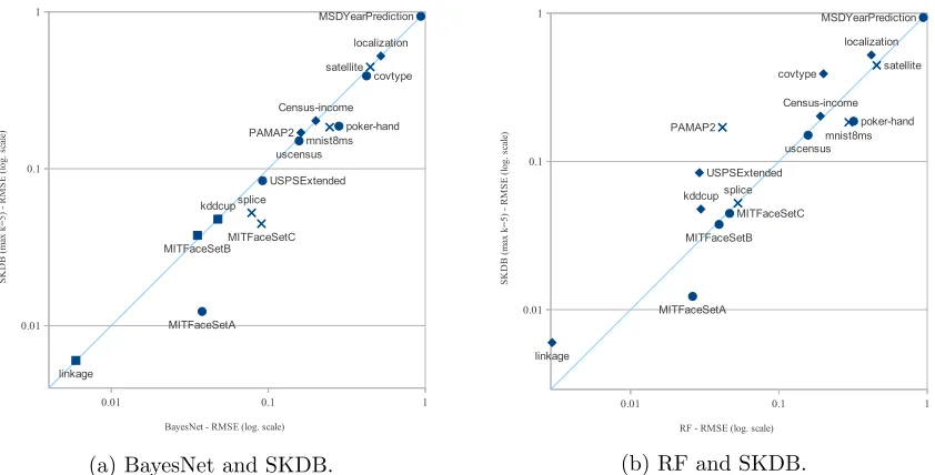
RMSE comparisons for all datasets for BayesNet and RF when compared with SKDB are shown in Figures 7a and 7b, where the points with an X symbol indicate those datasets for which sampling is required. While BayesNet is not competitive with SKDB, RF provides
competitive results for some datasets. PAMAP2 provides a notable case for which only a
sample of 2 millions out of 3.5 suffices for RF to provide better classification performance than SKDB using all the training data. This is however the only dataset for which RF learning from a sample can achieve lower RMSE than SKDB learning from all the data, the
reverse being true forsplice,mnistand satellite.
Figures 8a and 8b display the training and classification times per dataset for these classifiers compared to SKDB. For most datasets the in-core learners require substantially
more time for learning and classifying3.
100 1000 10000 100000
se
con
ds
)
BayesNet RF
0.1 1 10
tion ome kage type etA SetB nded
Tim
e (
s RF
SKDB
lo
cal
iza
t
C
ens
us
-i
nc
o
li
n
k
cov
t
M
ITFac
eS
MI
T
F
ac
eS
USPSExte
n
Datasets (a) Training Times
10 100
secon
d
s)
BayesNet RF
0.1 1
tion ome kage typ
e
etA SetB
n
ded
Tim
e (
s
SKDB
localiza
t
Census-i
n
co
li
n
k
cov
t
MITFaceS MITFace
S
USPSExte
n
Datasets (b) Classification Times
Figure 8: Time comparisons per dataset for BayesNet and RF against SKDB.
3.4 Global Comparison of All Classifiers
In this section we analyze how all the classifiers explored in this paper perform when they are compared as a set. Figure 9 plots the average rankings across all datasets, along with the standard deviation for each learner. This ranking corresponds to the ranking obtained when a Friedman test is conducted. In this analysis we present the 0-1 Loss performance of SKDB when it is optimized for RMSE, its average rank on 0-1 Loss improves marginally from 2.94 to 2.84 when it is instead optimized for 0-1 Loss.
When assessing the calibration of the probability estimates using RMSE, SKDB obtains
the lowest average rank of 2.53, followed by RF with 2.91 and KDB with 3.34 (very close
to those for VW and BayesNet). When assessing performance using 0-1 Loss, RF using its own internal discretization of numeric attributes enjoys an average advantage of 1 in rank over SKDB, and SKDB enjoys an average advantage of almost one third over VWLF.
We find NB at the other extreme on both measures, with average ranks 7.63 and 7.72
out of a total of 8 classifiers.
SKDB obtains in the worst case the 4.5th position (this half is due to a tie with
KDB-best-k) for the linkage dataset and the 4th position for census-income when ranked on
RMSE and the 4th position forMITFaceSetB and kddcup when ranked on 0-1 Loss.
On both measures the largest standard deviation is observed for VW, which usually ranks either very well or rather poorly among the datasets. Still, VW obtains the largest number of top 1 datasets for RMSE, with a total number of 7, against 5 for RF and 4 for SKDB. On 0-1 Loss, RF ranks first 8 times, VW 4 times and SKDB twice (one of those times being a tie with KDB-best-k).
A Friedman test (Demˇsar, 2006) was performed for the set of 8 classifiers, yielding
statistical difference for both measures. To identify where exactly these differences are found, we ran a set of posterior Nemenyi tests. These tests confirm the existence of two sets of algorithms in terms of performance on both RMSE and 0-1 Loss for these large datasets: on one hand NB, AODE and TAN; and on the other hand BayesNet, VW, KDB, RF and
SKDB. The Nemenyi tests4 showed significant differences for the second set of algorithms
over NB and AODE, and only RF and SKDB over TAN.
7.63
6.81
5.88
3.47 3.44 3.34
2.91
2.53
1 2 3 4 5 6 7 8
NB AODE TAN BayesNet VWLF KDB (best k) RF (Num) SKDB
Ranking
(a) RMSE
7.72
6.84
6.06
3.81
3.47
3.25
2.94
1.91
1 2 3 4 5 6 7 8
NB AODE TAN BayesNet KDB (best k) VWLF SKDB RF (Num)
Ranking
(b) 0-1 Loss
Figure 9: Ranking in terms of RMSE and 0-1 Loss for NB, TAN, AODE, KDB (with bestk),
SKDB, RF using numeric attributes, BayesNet and VW with a logistic function.
Even though the small number of datasets only allow tentative conclusions to be drawn, the following dataset characteristics appear to indicate a preference for one or another learning scheme.
• RF performs better on datasets with a small number of attributes.
• RF derives an advantage with respect to 0-1 Loss due to its internal discretization of
numeric values. It does not achieve the lowest RMSE or 0-1 Loss on any of the three
categorical only datasets poker-hand,PAMAP2 or splice.
• SKDB seems to cope well with high-dimensional datasets and datasets with more than
1 million points. However its complexity is quadratic with respect to the number of
Learner
T
ime (seconds)
NB TAN AODE KDB5 SKDB VWSF VWLF
0
5000
10000
15000
(a) Training Times
Learner
T
ime (seconds) − log. scale
NB TAN AODE KDB5 SKDB VWSF VWLF
50
100
200
500
1000
(b) Classification Times
Figure 10: Training and classification time comparisons for the out-of-core classifiers.
• VW appears to have an advantage for sparse numeric datasets.
A more detailed study of the domain of competence of these classifiers remains an important area for future work.
We can also analyze the performance of these classifiers with respect to the complexity of the decision function they provide. NB and linear regression, represented in this work by VW with linear features, are classifiers that learn linear decision boundaries. They have low variance and are particularly useful for small data quantity and sparse data. An extra
level of expressiveness is offered by AODE, KDB (k= 1), TAN and VWSF/VWLF (with
quadratic features); which produce quadratic decision functions. A2DE, KDB (k = 2)
and VWSF/VWLF (with cubic features) produce cubic decision functions. More generally,
AnDE and KDB can separate order-k(n) polynomially separable concepts (Jaeger, 2003).
These two families of classifiers provide a set of a spectrum of models of increasing com-plexity, allowing a fine-tuned trade-off between expressivity on the one hand, and efficiency of learning and guarding against overfitting on the other hand, that is, the well-known bias-variance trade off (Brain and Webb, 1999).
Figures 10a and 10b show the time comparison for the out-of-core classifiers considered:
namely NB, TAN, AODE, KDB withk= 5, SKDB and LRSGD with quadratic features in
Note that training SKDB with k = 5 (maximum) takes only a bit more time than
training KDB with k= 5. The classification time for KDB is slightly higher than SKDB’s
(since all attributes are considered). Training time for LRSGD with quadratic features and 3 passes (VWSF and VWLF), which are those that obtain comparable results with SKDB, are also higher, presumably because they have to compute all pairs of quadratic features as indicated above. Similar reasoning holds for classification time. We believe that the extra time for VW is also due to the need to binarize discrete features, that is, since
VW cannot deal with discrete attributes directly, v binary attributes are created for each
originally discrete attribute withv values; and also because of the one-against-all approach
required to handle classes with multiple labels. This overhead may be noticeable since we are using quadratic features. The time required for VWLF is much larger than VWSF, and in any case much larger both for training and testing than that for SKDB (specially note the logarithmic scale in Figure 10b).
4. Summary
We have developed an extension to KDB which performs discriminative attribute and best-k
selection using leave-one-out cross validation.
SKDB only requires a single extra pass over the training data compared to KDB. In return for this extra pass during training, it often increases prediction accuracy relative to
KDB with the best possible k, and always improves classification time (and space) by
re-ducing the number of attributes considered, which can be quite significant for some datasets
(for example forMITFaceSetC60%, 215.8 out of 361, of the attributes are selected
improv-ing the classification performance at the same time). It is embarrassimprov-ingly parallelizable. Furthermore, it can optimize any loss function that is a function over each training example
xof ˆp(Y,x) and yx, making it extremely flexible.
Due to its low bias, when datasets are large enough to avoid overfitting, SKDB attains lower error than the other in and out-of-core Bayesian network algorithms considered. It even provides competitive error compared to Random Forest, one of the most powerful in-core classification methods; and online linear and non-linear classifiers with stochastic gradient descent (that is, linear regression with quadratic and cubic features). Compared to the latter, it is in most cases substantially more efficient both at training and classification time. Further, it provides well-calibrated posterior class probability estimates.
Future directions for research include:
1. using only a sample of the data in the leave-one-out cross validation, in order to use more complex loss functions efficiently;
2. tackling SKDB’s tendency to overfit small training sets;
3. studying a customized selection of the different links and attributes in a discriminative manner, that is, different numbers of parents for different attributes and also discarded in an order that does not follow the conditional mutual information rank;
5. study of more appropriate loss functions for imbalanced datasets.
SKDB provides an efficient and effective solution to the problem of scalable low-bias learning. Its low bias allows it to capture and take advantage of the additional fine-detail that is inherent in very large data while its efficiency makes it feasible to deploy. SKDB thus sets new standards for classification learning from big data.
Acknowledgments
Appendix B. Implementation Details
All the experiments for the out-of-core algorithms have been carried out in a C++ software specially designed to deal with out-of-core classification methods. The following details in terms of implementation and configuration should be considered:
• 10-fold cross validation has been used.
• Equal frequency pre-discretization with 5 bins (EF5) has been utilized to discretize all
numeric attributes (except if otherwise specified5). We have observed that EF5 and
MDL (Minimum Description Length) (Fayyad and Irani, 1993) discretization provide the best results in approximately half of the datasets each, EF5 has been chosen because it is faster to perform than MDL, and also because it is not supervised and hence does not potentially provide the classifier with class information from the hold-out data when used for pre-discretization. Using a pre-fixed number of bins gives us the added advantage of not having to deal with a huge number of values per attribute created by MDL discretization in some cases.
• Missing values have been considered as a distinct value in all cases.
• The root mean square error is calculated exclusively on the true class label (different
from Weka’s implementation (Hall et al., 2009), where all class labels are considered).
• KDB’s implementation benefits from a tree structure that resembles an ADTtree
(Moore and Lee, 1998), sparseness is achieved by storing a NULL instead of a node for any query that matches zero records. In our case, to save the probability distri-bution of the different attributes once the structure has been determined, we build
a (distribution) tree for each attribute. Given, for example, attribute X4 that has
X0 and X3 as parents (in this order, and apart from the class), the counts (X4, Y)
are stored in the root node. The following level expands according to the number
of values of X0, which is the first parent, and store the counts for (X4, Y, X0). The
following level expands as for the number of values ofX3, which is the second parent,
and store the counts for (X4, Y, X0, X2), and so forth if there were more parents. Note
that as opposed to the ADTtree, all the parameters are stored, that is, more than strictly required, since a branch is created for each attribute value, when strictly one less branch would be sufficient to represent the model parameters. The reason to do that is not to overload classification time by having to explore and combine branches.
• Two combined techniques are considered for smoothing. In the first place, we use
m-estimates6 (Mitchell, 1997) as follows:
ˆ
p(xi|πxi) =
counts(xi, πxi) +
m
|Xi|
counts(πxi) +m
(4)
5. Only for the experiments on the antepenultimate row on Table 8 as specified.
6. Also known as Schurmann-Grassberger’s Law whenm= 1, which is a particular case of Lidstone’s Law (Lidstone, 1920; Hardy, 1920) withλ= 1
learner args lo caliz. cens-inc USPS MIT A MITB MSD Y co vt yp e MITC p ok er uscensus P AMAP kddcup link age mnist8 satellite splice NB 0 . 7106 ± 0 . 0007 0 . 4660 ± 0 . 0018 0 . 2256 ± 0 . 0026 0 . 0982 ± 0 . 0029 0 . 1394 ± 0 . 0014 0 . 9600 ± 0 . 0002 0 . 5103 ± 0 . 0013 0 . 2367 ± 0 . 0021 0 . 5801 ± 0 . 0006 0 . 2911 ± 0 . 0006 0 . 4647 ± 0 . 0006 0 . 1849 ± 0 . 0008 0 . 0125 ± 0 . 0006 0 . 4957 ± 0 . 0005 0 . 6540 ± 0 . 0002 0 . 0971 ± 0 . 0002 T AN 0 . 6321 ± 0 . 0014 0 . 2247 ± 0 . 0025 0 . 1153 ± 0 . 0022 0 . 0202 ± 0 . 0025 0 . 1213 ± 0 . 0020 0 . 9436 ± 0 . 0002 0 . 4862 ± 0 . 0008 0 . 2068 ± 0 . 0017 0 . 4987 ± 0 . 0006 0 . 1845 ± 0 . 0009 0 . 3232 ± 0 . 0007 0 . 0572 ± 0 . 0006 0 . 0081 ± 0 . 0009 0 . 3817 ± 0 . 0006 0 . 5424 ± 0 . 0003 0 . 1020 ± 0 . 0003 A ODE 0 . 6520 ± 0 . 0010 0 . 2932 ± 0 . 0020 0 . 1538 ± 0 . 0028 0 . 1001 ± 0 . 0036 0 . 1682 ± 0 . 0025 0 . 9459 ± 0 . 0002 0 . 4587 ± 0 . 0013 0 . 1564 ± 0 . 0014 0 . 5392 ± 0 . 0006 0 . 2154 ± 0 . 0010 ± 0 . 3881 ± 0 . 0008 0 . 0979 ± 0 . 0007 0 . 0120 ± 0 . 0005 0 . 3497 ± 0 . 0005 0 . 5783 ± 0 . 0003 0 . 1034 ± 0 . 0003 KDB k = 1 0 . 6501 ± 0 . 0012 0 . 2219 ± 0 . 0024 0 . 1125 ± 0 . 0025 0 . 0209 ± 0 . 0021 0 . 1291 ± 0 . 0019 0 . 9447 ± 0 . 0003 0 . 4709 ± 0 . 0026 0 . 1940 ± 0 . 0021 0 . 4987 ± 0 . 0005 0 . 1814 ± 0 . 0008 0 . 3276 ± 0 . 0007 0 . 0606 ± 0 . 0005 0 . 0082 ± 0 . 0009 0 . 3751 ± 0 . 0005 0 . 5506 ± 0 . 0003 0 . 0940 ± 0 . 0003 k = 2 0 . 5840 ± 0 . 0020 0 . 2064 ± 0 . 0021 0 . 0990 ± 0 . 0029 0 . 0126 ± 0 . 0019 0 . 0633 ± 0 . 0018 0 . 9393 ± 0 . 0002 0 . 4576 ± 0 . 0013 0 . 0906 ± 0 . 0012 0 . 4055 ± 0 . 0007 0 . 1677 ± 0 . 0008 0 . 2721 ± 0 . 0005 0 . 0497 ± 0 . 0008 0 . 0062 ± 0 . 0007 0 . 2922 ± 0 . 0004 0 . 5072 ± 0 . 0006 0 . 0953 ± 0 . 0002 k = 3 0 . 5485 ± 0 . 0020 0 . 2102 ± 0 . 0015 0 . 0928 ± 0 . 0025 0 . 0142 ± 0 . 0018 0 . 0468 ± 0 . 0018 0 . 9361 ± 0 . 0004 0 . 4399 ± 0 . 0015 0 . 0705 ± 0 . 0018 0 . 2859 ± 0 . 0011 0 . 1664 ± 0 . 0008 0 . 2290 ± 0 . 0004 0 . 0485 ± 0 . 0008 0 . 0060 ± 0 . 0006 0 . 2500 ± 0 . 0005 0 . 4769 ± 0 . 0004 0 . 1008 ± 0 . 0005 k = 4 0 . 5225 ± 0 . 0023 0 . 2107 ± 0 . 0012 0 . 0877 ± 0 . 0026 0 . 0514 ± 0 . 0031 0 . 0387 ± 0 . 0021 0 . 9383 ± 0 . 0006 0 . 4126 ± 0 . 0019 0 . 0616 ± 0 . 0016 0 . 2048 ± 0 . 0012 0 . 1601 ± 0 . 0007 0 . 1937 ± 0 . 0004 0 . 0478 ± 0 . 0008 0 . 0060 ± 0 . 0006 0 . 2169 ± 0 . 0005 0 . 4583 ± 0 . 0005 0 . 1084 ± 0 . 0003 k = 5 0 . 5225 ± 0 . 0023 0 . 2143 ± 0 . 0022 0 . 0839 ± 0 . 0034 0 . 1350 ± 0 . 0035 0 . 0841 ± 0 . 0023 0 . 9447 ± 0 . 0003 0 . 3903 ± 0 . 0020 0 . 0494 ± 0 . 0015 0 . 2842 ± 0 . 0011 0 . 1638 ± 0 . 0006 0 . 1697 ± 0 . 0004 0 . 0477 ± 0 . 0008 0 . 0060 ± 0 . 0006 0 . 1839 ± 0 . 0005 0 . 4448 ± 0 . 0004 0 . 0924 ± 0 . 0002 SKDB only k kmax = 5 0 . 5225 ± 0 . 0023 0 . 2064 ± 0 . 0021 0 . 0839 ± 0 . 0034 0 . 0126 ± 0 . 0019 0 . 0387 ± 0 . 0021 0 . 9361 ± 0 . 0004 0 . 3903 ± 0 . 0020 0 . 0494 ± 0 . 0015 0 . 2048 ± 0 . 0012 0 . 1601 ± 0 . 0007 0 . 1697 ± 0 . 0004 0 . 0477 ± 0 . 0008 0 . 0060 ± 0 . 0006 0 . 1839 ± 0 . 0005 0 . 4448 ± 0 . 0004 0 . 0924 ± 0 . 0002 bestk 4 2 5 2 4 3 5 5 4 4 5 5 3 . 8 5 5 5 SKDB k k = 1 0 . 6501 ± 0 . 0012 0 . 2054 ± 0 . 0014 0 . 1125 ± 0 . 0025 0 . 0207 ± 0 . 0020 0 . 0746 ± 0 . 0012 0 . 9446 ± 0 . 0003 0 . 4704 ± 0 . 0016 0 . 1227 ± 0 . 0014 0 . 4987 ± 0 . 0005 0 . 1540 ± 0 . 0007 0 . 3276 ± 0 . 0007 0 . 0606 ± 0 . 0005 0 . 0082 ± 0 . 0009 0 . 3751 ± 0 . 0005 0 . 5485 ± 0 . 0002 0 . 0527 ± 0 . 0002 k = 2 0 . 5840 ± 0 . 0020 0 . 2021 ± 0 . 0021 0 . 0990 ± 0 . 0029 0 . 0123 ± 0 . 0018 0 . 0574 ± 0 . 0011 0 . 9393 ± 0 . 0002 0 . 4576 ± 0 . 0013 0 . 0782 ± 0 . 0017 0 . 4055 ± 0 . 0007 0 . 1510 ± 0 . 0007 0 . 2721 ± 0 . 0005 0 . 0497 ± 0 . 0008 0 . 0062 ± 0 . 0007 0 . 2922 ± 0 . 0004 0 . 5065 ± 0 . 0004 0 . 0523 ± 0 . 0002 k = 3 0 . 5485 ± 0 . 0020 0 . 2056 ± 0 . 0016 0 . 0928 ± 0 . 0026 0 . 0144 ± 0 . 0021 0 . 0439 ± 0 . 0021 0 . 9361 ± 0 . 0004 0 . 4399 ± 0 . 0015 0 . 0596 ± 0 . 0020 0 . 2847 ± 0 . 0011 0 . 1508 ± 0 . 0007 0 . 2290 ± 0 . 0004 0 . 0485 ± 0 . 0008 0 . 0060 ± 0 . 0006 0 . 2500 ± 0 . 0005 0 . 4769 ± 0 . 0004 0 . 0523 ± 0 . 0002 k = 4 0 . 5225 ± 0 . 0023 0 . 2041 ± 0 . 0015 0 . 0877 ± 0 . 0026 0 . 0386 ± 0 . 0019 0 . 0376 ± 0 . 0026 0 . 9382 ± 0 . 0005 0 . 4126 ± 0 . 0019 0 . 0517 ± 0 . 0020 0 . 1868 ± 0 . 0012 0 . 1504 ± 0 . 0007 0 . 1937 ± 0 . 0004 0 . 0478 ± 0 . 0008 0 . 0060 ± 0 . 0006 0 . 2169 ± 0 . 0005 0 . 4583 ± 0 . 0005 0 . 0524 ± 0 . 0002 k = 5 0 . 5225 ± 0 . 0023 0 . 2070 ± 0 . 0015 0 . 0839 ± 0 . 0033 0 . 0552 ± 0 . 0032 0 . 0844 ± 0 . 0025 0 . 9447 ± 0 . 0004 0 . 3903 ± 0 . 0020 0 . 0446 ± 0 . 0020 0 . 1868 ± 0 . 0012 0 . 1505 ± 0 . 0007 0 . 1697 ± 0 . 0004 0 . 0477 ± 0 . 0008 0 . 0060 ± 0 . 0006 0 . 1839 ± 0 . 0005 0 . 4448 ± 0 . 0004 0 . 0526 ± 0 . 0002 SKDB kmax = 5 0 . 5225 ± 0 . 0023 0 . 2021 ± 0 . 0021 0 . 0839 ± 0 . 0033 0 . 0123 ± 0 . 0018 0 . 0376 ± 0 . 0026 0 . 9361 ± 0 . 0004 0 . 3903 ± 0 . 0020 0 . 0446 ± 0 . 0020 0 . 1868 ± 0 . 0012 0 . 1504 ± 0 . 0007 0 . 1697 ± 0 . 0004 0 . 0477 ± 0 . 0008 0 . 0060 ± 0 . 0006 0 . 1839 ± 0 . 0005 0 . 4448 ± 0 . 0004 0 . 0523 ± 0 . 0002 bestk 4 2 5 2 4 3 5 5 4 4 5 5 3 . 8 5 5 3 # of atts. 5 19 . 2 647 . 5 337 . 9 275 . 6 90 54 215 . 8 5 22 54 37 11 773 . 6 138 16 SKDB k (# of attributes selected) k = 1 5 7 584 . 9 354 . 9 17 80 . 5 45 . 8 59 10 11 54 38 . 2 11 772 . 2 75 13 k = 2 5 19 . 2 646 . 5 337 . 9 87 90 54 206 . 7 10 12 54 38 . 1 11 773 . 1 125 . 8 14 . 9 k = 3 5 18 648 . 1 356 . 1 271 . 3 90 54 209 . 6 5 22 54 37 . 6 11 774 . 2 138 16 k = 4 5 18 640 . 9 21 . 3 275 . 6 78 . 8 54 214 . 3 5 22 54 37 . 9 11 774 . 2 138 14 k = 5 5 18 647 . 5 18 359 . 3 81 . 2 54 215 . 8 5 22 54 37 11 773 . 6 138 13 n 5 41 676 361 361 90 54 361 10 67 54 41 11 784 138 141 Ba y esNet k = 5 0 . 5217 ± 0 . 0023 0 . 2009 ± 0 . 0016 0 . 0920 ± 0 . 0023 0 . 0379 ± 0 . 0136 0 . 0354 ± 0 . 0063 0 . 9369 ± 0 . 0004 0 . 4231 ± 0 . 0016 > 138G 0 . 2821 ± 0 . 0011 0 . 1573 ± 0 . 0008 0 . 1615 ± 0 . 0006 0 . 0477 ± 0 . 0007 0 . 0059 ± 0 . 0005 > 138G > 138G > 138G
Random Forest 100 trees 0 . 5194 ± 0 . 0024 0 . 1992 ± 0 . 0013 0 . 0338 ± 0 . 0010 0 . 0353 ± 0 . 0017 0 . 0566 ± 0 . 0012 > 138G 0 . 3478 ± 0 . 0018 0 . 0888 ± 0 . 0006 0 . 3190 ± 0 . 0028 0 . 1573 ± 0 . 0008 0 . 0962 ± 0 . 0012 0 . 0466 ± 0 . 0008 0 . 0060 ± 0 . 0007 > 138G > 138G > 138G