Evolutionary Model Type Selection for Global Surrogate Modeling
Dirk Gorissen [email protected]
Tom Dhaene [email protected]
Filip De Turck [email protected]
Ghent University - IBBT
Department of Information Technology (INTEC) Gaston Crommenlaan 8 bus 201
9050 Gent, Belgium
Editor: Melanie Mitchell
Abstract
Due to the scale and computational complexity of currently used simulation codes, global surrogate (metamodels) models have become indispensable tools for exploring and understanding the design space. Due to their compact formulation they are cheap to evaluate and thus readily facilitate visual-ization, design space exploration, rapid prototyping, and sensitivity analysis. They can also be used as accurate building blocks in design packages or larger simulation environments. Consequently, there is great interest in techniques that facilitate the construction of such approximation models while minimizing the computational cost and maximizing model accuracy. Many surrogate model types exist (Support Vector Machines, Kriging, Neural Networks, etc.) but no type is optimal in all circumstances. Nor is there any hard theory available that can help make this choice. In this paper we present an automatic approach to the model type selection problem. We describe an adaptive global surrogate modeling environment with adaptive sampling, driven by speciated evolution. Dif-ferent model types are evolved cooperatively using a Genetic Algorithm (heterogeneous evolution) and compete to approximate the iteratively selected data. In this way the optimal model type and complexity for a given data set or simulation code can be dynamically determined. Its utility and performance is demonstrated on a number of problems where it outperforms traditional sequential execution of each model type.
Keywords: model type selection, genetic algorithms, global surrogate modeling, function
approx-imation, active learning, adaptive sampling
1. Introduction
For many problems from science and engineering it is impractical to perform experiments on the physical world directly (e.g., airfoil design, earthquake propagation). Instead, complex, physics-based simulation codes are used to run experiments on computer hardware. While allowing scien-tists more flexibility to study phenomena under controlled conditions, computer experiments require a substantial investment of computation time. One simulation may take many minutes, hours, days or even weeks. A simpler approximation of the simulator is needed to make sensitivity analysis, visualization, design space exploration, etc. feasible (Forrester et al., 2008; Simpson et al., 2008).
con-centrates on the use of data-driven, global approximations using compact surrogate models (also known as emulators, metamodels or response surface models) in the context of computer exper-iments. The objective is to construct a high fidelity approximation model that is as accurate as possible over the complete design space of interest using as little simulation points as possible.
Once constructed, the global surrogate model (also referred to as a replacement metamodel1) is
reused in other stages of the computational science and engineering pipeline. So optimization is not the main goal, but rather a useful post processing step.
The primary users of global surrogate modeling methods are domain experts, few of which will be experts in the intricacies of efficient sampling and modeling strategies. Their primary concern is obtaining an accurate replacement metamodel for their problem as fast as possible and with minimal overhead. Model (type) selection, model parameter optimization, sampling strategy, etc. are of lesser or no interest to them. Thus, this paper explores an automated way to help answer the always recurring question from domain experts “Which approximation method is best for my data?”. An evolutionary algorithm is presented that combines automatic model type selection, automatic model parameter optimization, and sequential design exploration.
In the next Section we describe the problem of global surrogate modeling followed by an in depth discussion of the motivation for this work in Section 3. The core approach presented in this paper is discussed in Section 5 followed by a critical analysis in Section 6. Section 7 describes a number of surrogate modeling problems we shall use to demonstrate the proposed approach, followed by their discussion in Section 10 (the experimental setup is described in Section 9). We conclude in Section 12 with pointers to future work.
2. Global Surrogate Modeling
The mathematical formulation of the problem is as follows: approximate an unknown multivariate
function f : Ω 7→ Cn, defined on some domain Ω ⊂ Rd, whose function values f(X) =
{f(x1), ...,f(xk)} ⊂Cnare known at a fixed set of pairwise distinct sample points X={x1, ...,xk} ⊂
Ω. Constructing an approximation requires finding a suitable function s from an approximation
space S such that s :Ω7→Cn∈S and s closely resembles f as measured by some criterionξ, where
ξconstitutes three parts:
ξ= (Λ,ε,τ).
Λ is the generalization estimator, εthe error (or loss) function, andτ is the target value required
by the user. This means that the global surrogate model generation problem (i.e., finding the best
approximation s∗∈S) for a given set of data points D= (X,f(X))can be formally defined as
s∗=arg min
t∈Targ minθ∈ΘΛ(ε,st,θ,D) (1)
such that
Λ(ε,s∗t,θ,D)6τ
where st,θis the parametrizationθ(from a parameter spaceΘ) of s and st,θis of model type t (from
a set of model types T ).
The first minimization over t ∈T is the task of selecting a suitable approximation model type, that is, a rational function, a neural network, a spline, etc. This is the model type selection problem.
In practice, one typically considers only a single t∈T , though others may be included for
compari-son. Then given a particular approximation type t, the task is to find the hyperparameter assignment
θthat minimizes the generalization estimatorΛ(e.g., determine the optimal order of a polynomial
model). This is the hyperparameter optimization problem, though generally both minimization’s
are simply referred to as the model selection problem. Many implementations ofΛhave been
de-scribed: the hold-out, bootstrap, cross validation, jack-knife, Akaike’s Information Criterion (AIC),
etc. Different criteria may also be combined in a multi-objective fashion. In this caseξis really a
matrix
ξ=
Λ1 ε1 τ1 Λ2 ε2 τ2 ... ... ...
Λm εm τm
with m the number of objectives. A simple example is minimizing the average relative cross val-idation error together with the maximum absolute deviation in the training points. An additional
assumption is that f is expensive to compute. Thus the number of function evaluations|f(X)|needs
to be minimized and data points must be selected iteratively, at points where the information gain will be the greatest (Turner et al., 2007). Mathematically this means defining a sampling function
φ(Xj−1) =Xj, j=1, ..,N
that constructs a data hierarchy
X0⊂X1⊂X2⊂...⊂XN⊂X
of nested subsets of X , where N is the number of levels. X0is referred to as the initial experimental
design and is constructed using one of the many algorithms available from the theory of Design and
Analysis of Computer Experiments (Kleijnen et al., 2005). Once the initial design X0 is available
it can be used to seed the sampling functionφ. An important requirement ofφis to minimize the
number of sample points|Xj| − |Xj−1|selected each iteration, yet maximize the information gain
of each successive data level. Depending on the problem,φcan take into account different criteria
(non-linearity of the response, smoothness/uncertainty of the model, location of the optima, etc.). This process is referred to as adaptive sampling, active learning, model updating, or sequential design.
An important consequence of the adaptive sampling procedure is that the task of finding the best
approximation s∗(cfr. Equation 1) becomes a dynamic problem instead of a static one. Since the
optimal model parameters will change as the amount and distribution of data points changes. This of course makes the problem more difficult.
3. Motivation
While the mathematical formulation of global surrogate modeling is clear cut, its practical
im-plementation raises an obvious question: How should the minimization over t∈T and θ∈Θin
3.1 Problem 1: Model Type Selection
The first minimization over t∈T is the model type selection problem. Many model types exist:
rational functions, Artificial Neural Networks (ANN), Support Vector Machines (SVM), Gaussian Process (GP) models, Multivariate Adaptive Regression Splines (MARS), Radial Basis Function (RBF) models, projection pursuit regression, rational functions, etc.
3.1.1 BACKGROUND
From a theoretic standpoint, selecting the most suitable approximation method for a given response is a difficult problem that depends on the data characteristics (dimensionality, number of points, dis-tribution, noise level, periodicity, etc) and the application constraints (accuracy, smoothness, ability to capture poles or discontinuities, execution speed, interpretability, extrapolation requirements, etc). Different application domains prefer different model types. For example rational functions are widely used by the electrical engineering community (Deschrijver and Dhaene, 2005) while ANN are preferred for hydrological modeling (Solomatine and Ostfeld, 2008). Differences in model type usage are often due to practical reasons. This is particularly true in industrial settings. For example: the designer adheres to common practice within his field, the final application restricts the designer to one particular type (e.g., rational models for EM systems), or the expertise is not available to properly try other methods.
Of course, this need not always be the case. The choice of the metamodel type can also be
motivated by knowledge of the underlying physics2(Triverio et al., 2007) or by the special features
the model provides: for example the uncertainty prediction based on random process assumption in
Kriging methods3(Xiong et al., 2007). So remark there is no such thing as an inherently ‘good’ or
‘bad’ model. A model is only as good as the data it is based on and the expertise of the user that built it.
3.1.2 CLASSICAPPROACH
If multiple model types are considered, the classic approach is to simply to try out different types and select the best one according to one or more accuracy criteria. There is ample literature available that benchmarks model types in this way (Simpson et al., 2001; Jin et al., 2001; Queipo et al., 2005; Yang et al., 2005; Chen et al., 2006; Wang and Shan, 2007; Chung and Alonso, 2000; Gano et al., 2006; Gu, 2001; Santner et al., 2003; Lim et al., 2007; Fang et al., 2005; Gorissen et al., 2009c). But claims that a particular model type is superior to others should always be met with some skepticism. In order for the different benchmarking studies to be truly useful for a domain expert, the results of such studies must be collected and compiled into a general set of rules, recipe, or flowchart. To ease the discussion, let us denote such a compilation into a learning algorithm by L. L is then
essentially a classifier that can predict which model type t∈T to use based on data D and application
requirementsΓ:
2. Knowledge of the physics of the underlying system can make a particular model type to be preferred. For example, rational functions are popular for all kinds of Linear Time-Invariant systems since theory is available that can be used to prove that rational pole-residue models conserve certain physical quantities (Triverio et al., 2007).
L(D,Γ) =t.
When executed L should then be able to give a specific recommendation as to which model type to use for a given problem. This recommendation should be more specific than the general rules of thumb that are available now. Experience shows this to be exactly what an application engineer wants. However, constructing such a learner L for any but the most restricted class of problems is a daunting undertaking for obvious practical reasons. Firstly, deciding which problem/application features to train the classifier on is far from trivial. Also even if this is done, the number of features can be expected to be high thus gathering the necessary data (by manually solving Equation 1) to train L accurately will be very computationally expensive.
Secondly, as mentioned above, the success of a model type largely depends on the expertise of the user, the quality of the data, and even the quality of the software implementation of the technique. Neural networks are a good example in this respect. In the right hands they are able to perform very well on many problems. However, if poor choices are made with regard to training function, topology selection, generalization control, training parameters, software library, etc. they may seem to perform poorly. How to take into account this information in L?
Thirdly, a more fundamental problem with this approach is that data must be available in order for the reasoner to work. However, if only a simulation code is available (as is often the case) data must be collected, and the optimal data collection strategy that minimizes the number of points depends on the model type. Also, the optimal model type will change depending on how much data is available. One could argue to instead train L only on the data characteristics which are known in advance (e.g., dimensionality, noise level, etc.). The question is then again, which characteristics are most important? Furthermore, in many cases not much is known about the true behavior of the response thus there will typically not be enough information to train L accurately.
This brings us to the final point. A main reason for turning towards global surrogate modeling methods is that little is known about the behavior of the response (Simpson et al., 2008). The goal is to get insight into that behavior in a computationally cheap way by applying surrogate methods. Another reason why information about the data may be scarce is that the source of the data is confidential or proprietary and very little information is disclosed. In these situations using or training L becomes very difficult.
Finally, we must stress that we do not say that this problem is too difficult and not worth trying to solve. Indeed many such problems exist and are currently being tackled, particularly in medicine. Instead we argue that users of global surrogate modeling methods can benefit from a more dynamic approach that is flexible, can be easily applied to a wide range of different problems, can easily incorporate new fitting techniques and process knowledge, and naturally integrates with an adaptive data collection procedure. We shall revisit this point in sections 3.3 and 6.
3.2 Problem 2: Model Parameter Selection
Assuming the model type selection problem has been solved, there remains the model parameter
selection problem (the minimization overθ∈Θin Equation 1). For example, finding the optimal
C,εandσparameters in the case of RBF SVMs. This is the classic hyperparameter optimization
and usually it takes a great deal of experience to know how all parameters should be set. Sometimes this problem is solved through trial and error, but usually it is tackled as an optimization problem and classic optimization algorithms are used guided by a performance metric.
A huge amount of research has been done on this topic, particularly in the machine learning community (see Section 4). This particular problem is not the main focus of this work. Rather we are more interested in tackling the first problem.
3.3 Proposed Solution
While we are primarily interested in the first problem, the approach described in this paper naturally incorporates problem 2 as well. In both cases there is little theory that can be used as a guide. It is in this setting that the evolutionary approach can be expected to do well. We describe the application of a single GA with speciation to both problems: the selection of the surrogate type and the optimization of the surrogate model parameters (= hyperparameter optimization). In addition, we do not assume all data is available at once but must be sampled incrementally since it is expensive (active learning).
The idea is to maintain a heterogeneous population of surrogate model types and let them evolve cooperatively and dynamically with the changing data distribution. The details will be presented in Section 5 and a critique in Section 6. In addition, an implementation in the form of a Matlab toolbox
is available for download fromhttp://www.sumo.intec.ugent.be.
4. Related Work
The evolutionary generation of regression models for given input-output data has been widely stud-ied in the genetic programming community (Vladislavleva et al., 2009; Streeter and Becker, 2003; Yeun et al., 2004). Given a set of mathematical primitives (+, sin, exp, /, x, y, etc.) the space of sym-bolic expression trees is searched to find the best function approximation. The application of GAs to the optimization of model parameters of a single model type (homogeneous evolution) has also been common (Chen et al., 2004; Lessmann et al., 2006; Tomioka et al., 2007; Friedrichs and Igel, 2005; Zhang et al., 2000) and the extensive work by Yao (1999); Yao and Xu (2006). Integration with adaptive sampling has also been discussed (Busby et al., 2007). However, these efforts do not tackle the model type selection problem, they restrict themselves to a particular method (e.g., SVMs or neural networks). As Knowles and Nakayama (2008) state “Little is known about which types of model accord best with particular features of a landscape and, in any case, very little may be known to guide this choice.”. Likewise, Solomatine and Ostfeld (2008) note: “...it is important to stress that there are always situations when one model type cannot be applied or suffers from inadequa-cies and can be well complemented or replaced by another one”. Thus an algorithm to help solve this problem in a dynamic, automated way is very useful (Keys et al., 2007). This is also noticed by Voutchkov and Keane (2006) who compare different surrogate models for approximating each objective during optimization. They note that in theory their approach allows the use of a different model type for each objective. However, such an approach will still require an a priori model type selection and does not allow for dynamic switching of the model type or the generation of hybrids.
Based Optimization or Metamodel Assisted Optimization. A good overview reference is given by Eldred and Dunlavy (2006) and Queipo et al. (2005). For example, Lim et al. (2007) compare the utility of different local surrogate modeling techniques (quadratic polynomials, GP, RBF, ...) including the use of (fixed) ensembles, for optimization of computationally expensive simulation codes. Local surrogates are used together with a trust region framework to quickly and robustly identify the optimum. As noted in the introduction, the contrast with this work is that references such as Lim et al. (2007) are interested in the optimum and not the surrogate itself (they make only a “mild assumption on the accuracy of the metamodeling technique”). In addition the model parameters are taken as fixed and there is no integration with active learning. In contrast we place very strong emphasis on the surrogate model accuracy, the automatic setting of the hyperparameters, and the efficient sampling of the complete design space.
The work of Sanchez et al. (2006) and Goel et al. (2007) is more useful in our context since they provide new algorithms for generating an optimal set of ensemble members for a fixed set of data points (no sampling). Unfortunately, though, the parameters of the models involved must still be chosen manually. Nevertheless, their approaches are interesting, and can be used to further enhance the approach presented here. For example, instead of returning the single final best model, an optimal ensemble member selection algorithm can be used to return a potentially much better model based on the final population or Pareto front.
From machine learning the work in B. et al. (2004) is also related. The authors describe an interesting classification algorithm COMB that combines online an ensemble of active learners so as to expedite the learning progress in pool-based active learning. In their terminology an active learner is a combination of a model type and a sampling algorithm. A weighted ensemble of active learners is maintained and each learner is allowed to express interest in a pool of unlabeled training points. Depending on the interests of the active learners, an unlabeled point is selected, labeled by the teacher, and based on the added value of that point the different active learners are punished or rewarded. Internally the active learners are SVM models whose parameters are chosen manually. In principle, with a number of approximations one could adapt the algorithm to the regression case. If one then also included hyperparameter optimization, the result would be very similar to the SUMO-Toolbox (cfr. Section 5.2) configured with one or more of the Error, LRM, or EGO (Jones et al., 1998) sample selection algorithms, but without the ability to combine different criteria. However, a problem would be that COMB assumes a pool of unlabeled training data is given. However, when modeling a simulation code in regression no such pool is available. Some external algorithm would still be needed to generate it in order for COMB to work. COMB does also naturally allow for different model types but in a more static way than the algorithm in Section 5.3: there is no hyperparameter optimization, the number of each active learning type remains fixed (though the weights can change) leading to a potentially high computational cost, and hybrid models are not considered. The extension to the multi-objective case is also non-trivial. Of course COMB could be extended to incorporate such features, but the result would be very similar to the work presented here. Nevertheless, the specific scoring functions, probability weightings, and ensemble weight updates, seem very useful and could be implemented in the SUMO-Toolbox to complement the approach presented here.
are shown on various benchmarks. Unlike the GA approach, however, it is less straightforward to cater for multiple sub-populations, giving models room to mature independently before entering competition. The use of operators tuned to specific models is also difficult (to increase the search efficiency). In effect, the PSO approach takes a top-down view, using a high level encoding in a high dimensional space, a typical particle has 25 dimensions (Escalante et al., 2007). In contrast the GA approach is bottom up, the model specific operators result in a much smaller search space, different for each method (e.g., 1 for the spline models and 2 for the SVM models). This leads to a more efficient search requiring less fitness evaluations and facilitates the incorporation of prior knowledge. In addition, by using PSO there is no natural way of enabling hybrid solutions (ensem-bles) without extending the encoding and further increasing the search space. In contrast, the hybrid solutions arise very naturally in the GA framework and do not impact the search space of the other model types. The same is true of the extension to the multi-objective case, a very natural step in the GA case.
In sum, in by far the majority of the related work considered by the authors, speciation was always constrained to one particular model type, for example neural networks in Stanley and Mi-ikkulainen (2002). The model type selection problem was still left as an a-priori choice for the user. Or, if multiple model types are used, the hyperparameters are typically kept fixed and there is no tie-in with the active learning process.
5. Heterogeneous Evolution of Surrogate Models
This Section discusses how different surrogate models may be evolved cooperatively in order per-form model type selection.
5.1 Speciated Evolution
Since GAs are population-based they easily lend themselves to parallelism. The terms Parallel Genetic Algorithms (PGA) or Distributed Genetic Algorithms (DGA) refer to the case whenever the population is divided up in some way, be it to improve the computational efficiency or search efficiency. Unfortunately though, the terminology varies between authors and can be confusing (Nowostawski and Poli, 1999; Alba and Tomassini, 2002). From a biological standpoint it makes sense to consider speciation: genomes that differ considerably from the rest of the population are segregated and continue to evolve semi-independently, forming a new species.
Figure 1: Ring (left) and grid (right) migration topologies in the Island Model
5.2 Global Surrogate Modeling Control Flow
Before we can discuss the concrete implementation of the automatic model type selection algorithm it is important to revisit the general global surrogate modeling methodology described in Section 2. It is important to understand the general control flow since it forms the basis for the evolutionary algorithm described in the next Section.
The general methodology is as follows: Initially, a small initial set of samples is chosen accord-ing to some experimental design (e.g., Latin hypercube, Box-Behnken, etc.). Based on this initial set, one or more surrogate models are constructed and their hyperparameters optimized according to a chosen hyperparameter optimization algorithm (e.g., BFGS, Particle Swarm Optimization (PSO), Genetic Algorithm (GA), DIRECT, NSGA-II, etc.). Models are assigned a score based on one or more measures (e.g., cross validation, Akaike’s Information Criterion (AIC), etc.) and the optimiza-tion continues until no further improvement is possible. The models are then ranked according to their score and new samples are selected based on the best performing models and the behavior of the response (the exact criteria depend on the active learning algorithm used). The hyperparameter optimization process is continued or restarted intelligently and the whole process repeats itself until one of the following three conditions is satisfied: (1) the maximum number of samples has been reached, (2) the maximum allowed time has been exceeded, or (3) the user required accuracy has been met.
Recall that the adaptive sampling procedure has an important effect on the hyperparameter op-timization. The non-stationary data distribution makes the model parameter optimization surface dynamic instead of static (as is typically assumed).
A readily available implementation of the control flow described in this Section, and the one we shall use for the experiments in this paper, is available as the SUrrogate MOdeling Toolbox (SUMO
5.3 Algorithm
Algorithm 1 Automatic global surrogate modeling with heterogeneous evolution and active
learn-ing
01. X0=initialExperimentalDesign();
02. X=X0;
03 . f|X=evaluateSamples(X);
04 .T={t1, ...,th};
05. Mi=createInitialModels(ti,popsizei); i=1, ..,h
06. M=Sh
i=1Mi;
07 . while (ξ not reached) do
08. scores={}; gen=1;
09 . while ( termination_criteria not reached) do
10. foreachMi⊆M do
11. scoresi=fitness(Mi,X,f|X,ξ);
12. elite=sort([scoresi; Mi])|1:el;
13. parents=select(scoresi,Mi);
14. parentsxo=selectXOParents(parents,pc);
15. o f f springxo=crossover(parentsxo,ESdi f f,ESmax);
16. parentsmut=parents\parentsxo;
17. o f f springmut=mutate(parentsmut);
18. Mi=eliteSo f f springmutSo f f springxo;
19. scores=scoresi∪scores;
20. end
21. if(mod(gen,mi) =0)
22. M=migrate(M,scores,mf,md)
23. end
24. M=extinctionPrevention(M,Tmin);
25. gen=gen+1;
26. end
27 . Xnew=selectSamples(X,f|X,M);
28 . f|Xnew=evaluateSamples(Xnew);
29 . [X,f|X] =merge(X,f|X,Xnew,f|Xnew); 30 . end
31 . returnbestModel(M);
We now present the concrete GA for heterogeneous evolution as it is embedded (as a plugin) in the SUMO Toolbox. The speciation model used is the island model since we found it the most natu-ral way of evolving multiple model types while still allowing for hybrid solutions. The algorithm is based on the Matlab GADS toolbox and works as follows (see Algorithm 1 and reference (Gorissen, 2007) for more details): After the initial DOE has been calculated (cfr. the control flow in Section
5.2), an initial sub-population Miis created for each model type t∈T (i=1, ..,h). The exact
Subsequently, each deme is allowed to evolve according to an elitist GA. Parents are selected ac-cording a selection algorithm (e.g., tournament selection) and offspring undergo either crossover
(with probability pc) or mutation (with probability 1−pc). The models Miare implemented as
Mat-lab objects (with full polymorphism) thus each model type can choose its own representation and
mutation/crossover implementations (this implements the minimization overθ∈Θof Equation 1).
While mutation is straightforward, the crossover operator is more involved (see Section 5.5 below).
The fitness function calculates the quality of the model fit, according to criteriaξ. The current
deme population is then replaced with its offspring together with el elite individuals. Once every deme has gone through a generation, migration between individuals is allowed to occur at migration
interval mi, with migration fraction mf and migration direction md (a ring topology is used). The
migration strategy is as follows: the l= (|Mi| ·mf)fittest individuals of Mireplace the l worst
indi-viduals in the next deme (defined by md). As in Pei and Goodman (2001), migrants are duplicated,
not removed from the source population. Note that in this contribution we are primarily concerned with inter-model speciation (speciation as in different model types). Intra-model speciation (e.g., through the use of fitness sharing within one model type) is something which was not done but could easily be incorporated.
Once the GA has terminated, control passes back to the main global surrogate modeling algo-rithm of the SUMO Toolbox. At that point M contains the best set of models that can be constructed for the given data. If the accuracy of the models is sufficient the main loop terminates. If not, a new set of maximally informative sample points is selected based on several criteria (quality of the models, non-linearity of the response, etc.) and scheduled for evaluation. Once new simulations become available the GA is resumed.
Note that sample evaluation and model construction/hyperparameter optimization run in paral-lel. For clarity, algorithm 1 shows them running sequentially but this is not what happens in practice. In reality both are interleaved to allow an optimal use of computational resources.
5.4 Extinction Prevention
Initial versions of this algorithm exposed a major shortcoming, specifically due to the fact that
models are being evolved. Since not all data is available at once but trickles in,|Xj| − |Xj−1|samples
at a time, models that need a reasonable-to-large number of samples to work well will be at a huge disadvantage initially. Since they perform badly at first, they may get overwhelmed by other models who are less sensitive to this problem. In the extreme case where they are driven extinct, they will never have had a fair chance to compete when sufficient data does become available. They may
even have been the superior choice had they still been around.4 Therefore an Extinction Prevention
(EP) algorithm was introduced that ensures a model type can never disappear completely.
EP works by monitoring the population and each generation recording the number of
individ-uals of each model type. If this number falls below a certain threshold Tmin for a certain model
type, the EP algorithm steps in and ensures the model type has its numbers replenished up to the threshold. This is done by re-inserting the last models that disappeared for that type (making copies if necessary). The re-inserted models replace the worst individuals of the other model types (who do have sufficient numbers) evenly.
Strictly speaking, EP goes completely against the survival of the fittest principle in evolutionary algorithms. By using it we are manually working against selection, preserving model types which
give poor results at that point in time. However, in this setting it seems a fair measure to take (we do not want to risk loosing a model type completely) and improves results in most cases (see Section 10). At the same time it is straightforward to implement and understand, needing no special control parameters. All it has to ensure is that a species is never driven extinct.
5.5 Heterogeneous Recombination
The attentive reader will have noticed that one major problem remains with the implementation as discussed so far. The problem lies in the genetic operators, more specifically in the crossover operator. Migration between demes means that model types will mix. This means that a set of parents selected for reproduction may contain more than one model type. The question then arises: how to perform recombination between two models of completely different types. For example, how to meaningfully cross an Artificial Neural Network with a rational function? The solution we propose here is to use ensembles (behavioral recombination). If two models of different types are selected to recombine, an ensemble is created with the models as ensemble members. Thus, as soon as migration occurs, model types start mixing, and ensemble models arise as a result. These are treated as a distinct model type just as the other model types.
However, the danger with this approach is that the population may quickly be overwhelmed by large ensembles containing duplicates of the best models (as was noticed during initial tests). To counter this phenomenon we apply the similarity idea from Holland’s sharing concept (Holland, 1975). Individual models will try to mate only with individuals of the same type. Only in the case where selection has made this impossible shall different model types combine to form an ensemble.
In addition we enforce a maximum ensemble size ESmaxand require that ensemble members must
differ ESdi f fpercent in their response (their ‘behavior’). This is calculated by evaluating the models
on a dense grid.
This leaves us with only three cases left to explain:
1. ensemble - ensemble recombination: a single-point crossover is made between the ensemble member lists of each model (note that the type of the ensemble members is irrelevant)
2. ensemble - model recombination: the model replaces a randomly selected ensemble member
with probability pswapor gets absorbed into the ensemble with probability 1−pswap
(respect-ing ESmaxand ESdi f f).
3. ensemble mutation: one ensemble member is randomly deleted
Besides enabling hybrid solutions, using ensembles has the additional benefit of allowing a model to lie ‘dormant’ in an ensemble with the possibility of re-emerging later (e.g., if after mutation only one ensemble member remains). Note that, in contrast to Lim et al. (2007) for example, the type of the ensemble members is not fixed in any way but varies dynamically.
ensemble is that it works in all cases: It makes no assumption on the model types involved, nor does it mandate any changes to the models or training algorithms (for example, like negative corre-lation learning) since this is not always possible (e.g., when using proprietary, application specific, modeling code).
5.6 Multi-objective Model Selection
A crucial aspect of the model generation algorithm is the choice of a suitable criteriaξ. In
prac-tice it turns out that selecting an appropriate function forΛ,εand a target value for τis difficult.
Particularly if little is known about the structure of the response. This is related to the “The 5 percent problem” (Gorissen et al., 2009b). The fundamental reason for this difficulty is that an approximation task inherently involves multiple, conflicting, criteria (Li and Zhao, 2006). Thus a multi-objective approach is very useful here since it enables the use of multiple criteria during the hyperparameter optimization process (see Jin and Sendhoff 2008 for an excellent overview of this line of research).
Secondly, it is not uncommon that a simulation engine has multiple outputs that all need to be modeled (Conti and O’Hagan, 2007). The direct approach is to model each output independently with separate models (possibly sharing the same data). This, however, leaves no room for trade-offs nor gives any information about the correlation between different outputs. Instead of performing two modeling runs (doing a separate hyperparameter optimization for each output) both outputs can be modeled simultaneously if models with multiple outputs are used in conjunction with a multi-objective optimization routine.
In both cases such a multi-objective approach can be integrated with the automatic surrogate model type selection algorithm described here. This means that the best model type can vary per criteria or, more interestingly, that it enables automatic selection of the best model type for each output without having to resort to multiple runs. A full discussion of these topics is out of scope for this paper. However, details and some initial results can already be found in Gorissen et al. (2009a) and Gorissen et al. (2009b).
6. Critique
The algorithm presented so far has a number of strengths and weaknesses. The obvious advantage is the ability to perform automatic selection of the model type and complexity for a given data source (no need to do multiple parallel runs or train a complex classifier). In addition the algorithm is generic in that it is independent of the data origin (application), model type, and data collection strategy. New approximation methods can easily be incorporated without changing the algorithm. Problem specific knowledge and model type specific optimizations based on expert knowledge can also be incorporated if needed (i.e., by customizing the genetic operators). Furthermore, the algo-rithm naturally integrates with the data collection strategy, allowing the best model type to change dynamically and naturally allows for hybrid solutions. Finally, it naturally extends to the multi-objective case (Section 5.6) and can be easily parallelized to allow for faster computations (though the computational cost is still outweighed by the simulation cost).
matter. Formulating theoretical foundations in order to come to convergence guarantees for GAs is a difficult undertaking and has been the topic of intense research ever since their inception in the late 80s. Characterizing the performance of genetic algorithms is complex and depends on the application domain as well as the implementation parameters (Rawlins, 1991). Most theoretic work has been done on schema theorems for the Canonical Genetic Algorithm (CGA), which try to prove convergence in a simplified framework using a binary representation. However prediction of the future behavior of a GA turns out to be very difficult and much controversy remains over the useful-ness of these theorems (Poli, 2001; Goldberg, 1989). Theoretical work on other classes of GAs or using specific operators has also been done (Nakama, 2008; Neubauer, 1997; Rawlins, 1991; Qi and Palmieri, 1994a,b) but is unfortunately of little practical use here. For example, the work in Anken-brandt (1990) requires the calculation of fitness ratios, but this is impractical (and computationally expensive) to do in this situation and the results will vary with the application.
Thus, for the purposes of this paper a full mathematical treatment of algorithm 1 and its conver-gence is out of scope. Due to the island model, sampling procedure, and heterogeneous representa-tion/operators used, such a treatment will be far from trivial to construct and distract from the main theme of the paper. In addition its practical usefulness would remain questionable due to the many assumptions that will be required. However, gaining a deeper theoretical insight into the robustness of the algorithm is still very important. A sensitivity study of the main GA parameters involved will shed more light on this issue.
Theoretical remarks aside, the authors have found that in practice the approach works quite well. If reasonable population sizes are used together with migration and the extinction prevention algorithm described in Section 5.4, the results of the algorithm are quite robust and give useful re-sults and insights into the modeling problem. Besides the rere-sults given in this paper, good rere-sults have also been reported on various real world problems from aerodynamics (Gorissen et al., 2009a), electronics (Gorissen et al., 2008a), hydrology (Couckuyt et al., 2009), and chemistry (Gorissen, 2007).
In sum, this approach is useful if: little information is known about the expected structure of the response, if it is unclear which model type is most suited to the problem, data is expensive and must be collected iteratively, and hybrid solutions are useful. In other cases, for example it is clear from a priori knowledge which model type will be the most suitable (e.g., based on existing rules of thumb for a well defined, restricted problem), this approach should not be applied, save as a comparison.
7. Test Problems
We now consider five test problems to which we apply the heterogeneous GA (from now on ab-breviated by HGA). The objective is to validate if the best model type can indeed be determined automatically, and in a way that is cheaper and better than the simple brute force method: doing multiple, single model type runs in parallel. The problems include 2 predefined mathematical func-tions, and real-world problems from electronics and aerodynamics.
We also hope to see evidence of a ‘battle’ between model types. While initially one species may have the upper hand, as more data becomes available (dynamically changing hyperparameter optimization landscape) a different species may become dominant. This should result in clearly noticeable population dynamics, a kind of oscillatory stage before convergence. We briefly discuss each of the test problems in turn.
7.1 Ackley Function (AF)
The first test problem is Ackley’s Path, a well known benchmark problem from optimization. Its mathematical definition for d dimensions is:
F(~x) = −20·exp −0.2 s
1 d·
d
∑
i=1x2i !
−exp 1
d ·
d
∑
i=1cos(2π·xi)
!
+20+e
with xi∈[−2,2]for i=1, ...,d. For easy visualization we take d=2. For this function a validation
set and a test set of 5000 random points each is available. Although this is a function from opti-mization we are not interested in optimizing it, rather in reproducing it using a regression method with minimal data.
7.2 Kotanchek Function (KF)
The second predefined function is the Kotanchek function (Smits and Kotanchek, 2004). Its mathe-matical definition is given as:
F(x1,x2,u1,u2,u3) =
e−x22
1.2+x21+ε
with x1∈[−2.5,1.5], x2∈[−1.0,3.0], and withεuniform random simulated numeric noise with
mean 0 and variance 10−4. As you can see only the first two variables are relevant. For this function
a validation set and a test set of 5000 scattered points each is available.
7.3 EM Example (EE)
The fourth example is a 3D Electro-Magnetic (EM) simulator problem (Lehmensiek, 2001). Two perfectly conducting round posts, centered in the E-plane of a rectangular waveguide, are modeled, as shown in Figure 2. The 3 inputs to the simulation code are: the signal frequency f , the diameter of the posts d, and the distance between the two posts w. The outputs are the complex reflection and
transmission coefficients S11and S21. The simulation model was constructed for a standard WR90
rectangular waveguide with f ∈[7 GHz, 13 GHz], d∈[1 mm, 5 mm] and w∈[4 mm, 18 mm]. In
addition, a 253data set is available for testing purposes.
7.4 LGBB Example (LE)
Figure 2: Cross sectional view and top view of the inductive posts (Lehmensiek, 2001)
(a) LGBB geometry (Rogers et al., 2003) (b) Lift plotted as a function of speed and an-gle of attack with side-slip anan-gle fixed to zero (Gramacy et al., 2004).
Figure 3: LGBB Example
at significantly lower launch costs, improved reliability and maintainability. The vehicle is a three-stage system with a reusable first three-stage and expendable upper three-stages. The reusable first three-stage booster, which glides back to launch site after staging around Mach 3 is named the Langley Glide-Back Booster (LGBB). In particular, NASA is interested in the aerodynamic characteristics of the LGBB from subsonic to supersonic speeds when the vehicle reenters the atmosphere during its gliding phase.
Figure 3b shows the lift response plotted as a function of speed (Mach) and angle of attack (alpha) with the side-slip angle (beta) fixed at zero. The ridge at Mach 1 separates subsonic from supersonic cases. From the figure it can be seen there is a marked phase transition between flows at subsonic and supersonic speeds. This transition is distinctly linear and may even be non-differentiable or non-continuous (Gramacy et al., 2004). Given the computational cost of the CFD solvers, the LGBB example is an ideal application for metamodeling techniques. Unfortunately access to the original simulation code is restricted. Instead a data set of 780 points chosen adaptively according to the method described in Gramacy et al. (2004) was used.
7.5 Boston Housing Example (BH)
The Boston Housing data set contains census information for 506 housing tracts in the Boston area and is a classic data set used in statistical analysis. It was collected by Harrison et al. and described in Harrison and Rubinfeld (1978). In the case of regression the objective is to predict the Median value of owner-occupied homes (in $1000’s) from 13 input variables (e.g., per capita crime rate by town, nitric oxide concentration, pupil-teacher ratio by town, etc.).
8. Model Types
For the tests the following model types are used: Artificial Neural Networks (ANN), rational func-tions, RBF models, Kriging models, LS-SVMs, and for the AF example: also smoothing splines. For the EM example only the model types that support complex valued outputs directly (rational functions, RBF, Kriging) were included. Each type has its own representation and genetic operator implementation (thanks to the polymorphism as a result of the object oriented design). As stated in subsection 5.5 the result of a heterogeneous recombination will be an averaged ensemble. So in total up to seven model types will be competing to approximate the data. Remember that all model parameters are chosen automatically as part of the GA. No user input is required, the models and data points are generated automatically.
The ANN models are based on the Matlab Neural Network Toolbox and are trained with Leven-berg Marquard backpropagation with Bayesian regularization (MacKay; Foresee and Hagan, 1997) (300 epochs). The topology and initial weights are determined by the GA. When run alone (without the HGA) this results in high quality models with a much faster run time than training the weights by evolution as well. Nevertheless, the high level Matlab code and complex training function do make the ANNs much slower than any of the other model types.
The LS-SVM models are based on the implementation from Suykens et al. (2002), the kernel
type is fixed to RBF, leaving c andσto be chosen by the GA. The Kriging model implementation
is based on Lophaven et al. (2002) (except for the EM example) and the correlation parameters are set by the GA (the regression function is set to linear and the correlation function to Gaussian). The RBF models (and the Kriging models for the EM example, since the data is complex valued) are based on a custom implementation where the regression function, correlation function, and correla-tion parameters are all evolved. The racorrela-tional funccorrela-tions are also based on a custom implementacorrela-tion, the free parameters being the orders of the two polynomials, the weights of each parameter, and which parameters belong in the denominator. The spline models are based on the Matlab Splines Toolbox and only have one free parameter: the smoothness.
together in a single algorithm. Thus a full explanation of the virtues of each model types, as well as the representation and genetic operators used is out of scope for this paper and would consume too much space. Details can be found in Gorissen (2007) or in the implementation that is available as part of the SUMO Toolbox.
9. Experimental Setup
The following subsections describe the configuration settings used (and their motivation) for per-forming the experiments.
9.1 Sample Selection Settings
For the LE and BH examples only a fixed, small size, data set is available. Thus, selecting samples adaptively makes little sense. So for these examples the adaptive sampling loop was switched off. For the other examples the settings were as follows: an initial optimized Latin hypercube design, using the method from Ye et al. (2000), of size 50 is used augmented with the corner points. Mod-eling is allowed to commence once at least 90% of the initial samples are available. Each iteration a maximum of 50 new samples are selected using the Local Linear (LOLA) adaptive sampling algo-rithm (Crombecq et al., 2009). LOLA identifies new sample locations by making a tradeoff between eploration (covering the design space evenly) and exploitation (concentrating on regions where true response is nonlinear). LOLA’s strengths are that it scales well with the number of dimensions, makes no assumptions about the underlying problem or surrogate model type, and works in both
theRandCdomains. LOLA is able to automatically identify non-linear regions in the domain and
sample these more densely compared to more linear, ‘flatter’ regions.
By default LOLA does not rely on the (possibly misleading) approximation model, but only on the true response. This is useful here since it allows us to consider the model selection results inde-pendent from the sample selection settings. I.e., the final distribution of points chosen by LOLA is the same across all runs and model types. This means that any difference in performance between models can not be due to differences in sample distribution. However, in many cases it may be desirable to also include information about the surrogate model itself when choosing potential sam-ple locations. In this case the LOLA algorithm can be combined with one or more other sampling criteria that do depend on model characteristics (for example the Error, LRM, and EGO algorithms available in SUMO).
9.2 GA Settings
The GA is run for a maximum of 15 generations between each sampling iteration (after sampling, the GA continues with the final population of the previous iteration). It terminates if one of the following conditions is satisfied: (1) the maximum number of generations is reached, or (2) 8
gen-erations with no improvement. The size of each deme is set to 15. The migration interval miis set
to 7, the migration fraction mf to 0.1 and the migration direction is both (copies of the mf best
indi-viduals from island i replace the worst indiindi-viduals in islands i−1 and i+1). A stochastic uniform
RRSE(yi,y˜i) =
s
∑n
i=1(yi−y˜i)2
∑n
i=1(yi−y¯)2
where yi,y˜i,y are the true, predicted, and mean true response values respectively. Intuitively the¯
RRSE indicates how much better an approximation is than the most simple approximation possible (the mean) (Ganser et al., 2007). In the case of the BH and LE examples no separate validation set is available, instead 20% of the available data is reserved for this purpose (taking care to ensure the validation set is representative of the full data set by maximizing the minimum distance between validation points). Note that we are using a validation set since it is cheap and we have enough data available. In the case where data is scarce we would most likely use the more expensive k-fold cross validation as a fitness measure. This is the case for the EM example.
The remaining parameters are set as follows: pm=0.2,pc=0.7,k=1,pswap=0.8,el=1,ESmax=
3,ESdi f f =0.1,Tmin=2. The random generator seed was set to Matlab’s default initial seed.
9.3 Termination Criteria
In case of adaptive modeling only (no sample selection), the objective is to see what the most accu-rate model is that can be found in a limited period of time (= a typical use case). Thus the required accuracy (= target fitness value) is set to 0. For the LE the timeout is set to 180 minutes. For the BH example the timeout is significantly extended to 1200 minutes. Given the high dimensionality, the noise and discontinuities in the input domain it is a hard problem to fit accurately. In this case we are more interested to see how the population would evolve over such an extended period of time.
In case of adaptive sampling, the criteria are: a target accuracy (RRSE) of 0.01, and for the AF example a maximum number of 500 data points is enforced (to see what performance can be reached with a limited sample budget).
9.4 Others
Each problem was modeled twice with the heterogeneous evolution algorithm (once with EP=true,
once with EP= f alse) and once with homogeneous evolution (a single model type run for each
model type in the HGA). To smooth out random effects each run was repeated 15 times. This resulted in a total of 516 runs which used up a total of at least 130 days worth of CPU time (excluding initial tests and failed runs). All experiments were run on CalcUA, the cluster available at the University of Antwerp, which consists of 256 Sun Fire V20z nodes (dual AMD Opteron with 4 or 8 GB RAM), running SUSE linux, and Matlab 7.6 R2008a. Due to space considerations, only the results for the S11 (EE), and lift (LE) outputs are considered in this paper. For all examples the input
space is normalized to the interval[−1,1].
10. Discussion
We now discuss the results of each problem separately in the following subsections.
10.1 Ackley Function
1 2 3 4 5 6 7 8 9 101112131415 0 10 20 30 40 50 60 70 80 90
Number of runs
Number of models (out)
avg: [ 7.33e−01 00 00 00 5.81e+01 3.11e+01 00 ] std: [ 2.84e+00 00 00 00 4.31e+01 4.33e+01 00 ]
Ensemble Spline Kriging Rational RBF LS−SVM ANN
1 2 3 4 5 6 7 8 9 101112131415 0 10 20 30 40 50 60 70 80 90
Number of runs
Number of models (out)
avg: [ 5.47e+00 02 02 02 6.83e+01 8.27e+00 02 ] std: [ 7.74e+00 00 00 00 2.24e+01 1.90e+01 00 ]
Ensemble Spline Kriging Rational RBF LS−SVM ANN
Figure 4: AF: Composition of the final population (Left: EP=false, Right: EP=true)
1 2 3 4 5 6 7 8 9 101112131415 0 10 20 30 40 50 60 70 80 90 100
Number of runs
Percantage of test samples (out)
avg: [ 00 6.13e−02 1.11e+01 5.33e+01 3.04e+01 5.09e+00 ] std: [ 00 8.60e−02 1.07e+01 1.30e+01 1.72e+01 4.21e+00 ]
e >= 1e0 1e0 > e >= 1e−1 1.e−1 > e >= 1e−2 1e−2 > e >= 1e−3 1.e−3 > e >= 1e−4 e < 1e−4
1 2 3 4 5 6 7 8 9 101112131415 0 10 20 30 40 50 60 70 80 90 100
Number of runs
Percantage of test samples (out)
avg: [ 00 1.33e−03 2.16e+00 3.69e+01 5.02e+01 1.08e+01 ] std: [ 00 5.16e−03 7.12e−01 4.34e+00 3.08e+00 2.31e+00 ]
e >= 1e0 1e0 > e >= 1e−1 1.e−1 > e >= 1e−2 1e−2 > e >= 1e−3 1.e−3 > e >= 1e−4 e < 1e−4
Figure 5: AF: Error histogram of the final best model in each run (Left: EP=false, Right: EP=true)
deviation over all runs. The first element of each vector corresponds to the first (top) legend entry. The error histogram of the final model of each run on the test data is shown in Figure 5. The population evolution for the run that produced the best model in both cases is shown in Figure 6. Figure 7 then depicts the evolution of the relative error (calculated according to Equation 2) on the test set as modeling progresses (again in both cases, for the run that produced the best model). The lighter the regions in Figure 7, the larger the percentage of test samples that have low relative error (RE) (according to Equation 2).
RE(y,y˜) =|y−y˜|
1+|y|. (2)
Finally, a summary of the results for each run is shown in Table 1. The table shows the number
0 50 100 150 200 0 10 20 30 40 50 60 70 80 90 Generation
Number of models (out)
Ensemble Spline Kriging Rational RBF LS−SVM ANN
0 50 100 150 200
0 10 20 30 40 50 60 70 80 Generation
Number of models (out)
Ensemble Spline Kriging Rational RBF LS−SVM ANN
Figure 6: AF: Population evolution of the best run (Left: EP=false, Right: EP=true)
100 200 300 400 500 0 10 20 30 40 50 60 70 80 90 100
Number of samples
Percantage of test samples (out)
e >= 1e0 1e0 > e >= 1e−1 1.e−1 > e >= 1e−2 1e−2 > e >= 1e−3 1.e−3 > e >= 1e−4 e < 1e−4
100 200 300 400 0 10 20 30 40 50 60 70 80 90 100
Number of samples
Percantage of test samples (out)
e >= 1e0 1e0 > e >= 1e−1 1.e−1 > e >= 1e−2 1e−2 > e >= 1e−3 1.e−3 > e >= 1e−4 e < 1e−4
Figure 7: AF: Error evolution of the best run (Left: EP=false, Right: EP=true)
Method |X| σ V ERRSE¯ σ T ERRSE¯ σ time (min)¯ σ
ANN 4.973E+02 1.759E+01 1.308E-02 3.428E-03 1.298E-02 3.456E-03 1.810E+02 3.176E+01 Kriging 5.263E+02 1.193E+01 2.014E-02 4.266E-03 2.038E-02 4.521E-03 7.256E+01 9.194E+00 LS-SVM 5.202E+02 1.200E+01 1.367E-02 2.262E-03 1.375E-02 2.314E-03 3.995E+01 3.276E+00 Rational 5.170E+02 1.023E+01 1.881E-01 5.854E-02 1.861E-01 5.932E-02 2.033E+01 2.221E+00 RBF 5.193E+02 1.540E+01 1.326E-02 2.365E-03 1.324E-02 2.313E-03 4.371E+01 4.133E+00 Splines 5.308E+02 1.360E+01 2.471E-02 5.660E-03 2.428E-02 5.404E-03 4.292E+01 4.984E+00 HGAEP=f alse 5.055E+02 6.512E+00 3.142E-02 1.777E-02 3.094E-02 1.711E-02 2.366E+02 1.566E+02
−1 −0.5
0 0.5
1
−1 −0.5 0 0.5 1 0 1 2 3 4 5 6 7 8
x y
out
Figure 8: AF: normalized plot of the best model overall (HGAEP=true)
experiment. All entries are averaged over 15 runs with the standard deviation shown in the adjacent column. The plot of the best model found overall is shown in Figure 8.
Regarding the composition of the final population in Figure 4, we see that the results are some-what mixed for EP=false. In some runs RBF models perform best, in others LS-SVM models. This is also reflected in the corresponding error histogram plot in Figure 5. The quality of the best model found in each run differs considerably between runs. In contrast, for EP=true, the results are more clear cut, RBF models dominate in 14 of the 15 runs. This already demonstrates the usefulness of extinction prevention. Due to randomness in the initial population and genetic operators a model type may be driven extinct, unable to return. EP prevents this. In this particular case LS-SVM models generally perform best initially, pushing the RBF models out of the population. However, as more data becomes available (active learning), and as the hyperparameter optimization continues, superior RBF models are discovered and quickly take over the population. This is also nicely shown in Figure 6. In both cases the RBF models are driven out of the population around generation 50. Though in the EP=true case the RBF models are able to make a re-appearance around generation 100.
Of course nothing prevents this process from recurring. The fact that the optimal solution changes with time is not a disadvantage and should actually be expected since the optimization landscape is dynamic (due to the incremental sampling). Without EP these oscillations are impossi-ble and everything depends on the initial conditions. As a result the danger of converging to a poor local optimum is considerably greater. Given the form of the Ackley function, we should really not be surprised that the RBF models end on top. The different radial basis functions that make up the RBF model (= a local model) can be expected to match up quite well with the ‘bumps’ of the Ackley function.
1 2 3 4 5 6 7 8 9 101112131415 0
10 20 30 40 50 60 70 80 90 100
Number of runs
Percantage of test samples (noisy)
avg: [ 00 00 00 4.17e−01 4.71e+01 5.25e+01 ] std: [ 00 00 00 5.27e−01 9.90e+00 1.02e+01 ]
e >= 1e0 1e0 > e >= 1e−1 1.e−1 > e >= 1e−2 1e−2 > e >= 1e−3 1.e−3 > e >= 1e−4 e < 1e−4
1 2 3 4 5 6 7 8 9 101112131415 0
10 20 30 40 50 60 70 80 90 100
Number of runs
Percantage of test samples (noisy)
avg: [ 00 00 00 1.48e−01 3.10e+01 6.89e+01 ] std: [ 00 00 00 2.40e−01 8.89e+00 8.88e+00 ]
e >= 1e0 1e0 > e >= 1e−1 1.e−1 > e >= 1e−2 1e−2 > e >= 1e−3 1.e−3 > e >= 1e−4 e < 1e−4
Figure 9: KF: Error histogram of the final best model in each run (Left: EP=false, Right: EP=true)
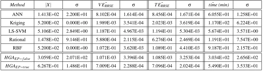
Method |X| σ V ERRSE¯ σ T ERRSE¯ σ time (min)¯ σ
ANN 1.413E+02 2.200E+01 8.102E-04 1.614E-04 8.456E-04 1.671E-04 6.055E+01 1.258E+01 Kriging 5.200E+02 0.000E+00 1.989E-03 3.541E-04 2.023E-03 3.619E-04 1.170E+02 6.224E+01 LS-SVM 5.106E+02 2.849E+00 1.187E-01 4.967E-03 1.194E-01 5.304E-03 5.674E+01 3.571E+00 Rational 1.478E+02 9.146E+01 5.880E-04 2.115E-04 6.276E-04 2.469E-04 1.191E+01 7.547E+00 RBF 5.200E+02 0.000E+00 1.072E-01 3.620E-03 1.089E-01 4.410E-03 9.187E+01 2.157E+01 HGAEP=f alse 3.059E+02 2.071E+02 1.071E-03 3.396E-04 1.085E-03 3.253E-04 3.034E+02 2.656E+02
HGAEP=true 6.267E+01 1.486E+01 7.009E-04 2.288E-04 7.096E-04 2.024E-04 5.490E+01 3.533E+01 Table 2: KF: Comparison with homogeneous evolution
The natural question that remains, is how do these results compare with simply doing multiple homogeneous evolution (single model type, using the same GA settings) runs, one for each type separately? Those results are shown in Table 1. Studying the table we see that the HGA compares favorably. The accuracy of the final models are the essentially the same as those found by the best performing single model type run, while the variance on the results tends to be lower (EP=true). Of course this is paid for by an increase in computation time due to the increased population size of the HGA. Still, the HGA has a factor of 6 larger population size (90 vs 15) but requires only double the running time of the best performing homogeneous run (ANN). Also the total HGA running time is still less than the combined run time of all homogeneous runs.
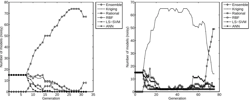
10.2 Kotanchek Function
The composition of the final population and final error histograms for each run are shown in Figures 9 and 10. The population evolution and corresponding error evolution for the best run are shown in Figures 11 and 12. The comparison with homogeneous evolution is shown in Table 2.
1 2 3 4 5 6 7 8 9 101112131415 0 10 20 30 40 50 60 70 80
Number of runs
Number of models (noisy)
avg: [ 6.27e+00 4.96e+01 1.91e+01 6.67e−02 00 00 ] std: [ 1.43e+01 3.38e+01 3.28e+01 2.58e−01 00 00 ]
Ensemble Kriging Rational RBF LS−SVM ANN
1 2 3 4 5 6 7 8 9 101112131415 0 10 20 30 40 50 60 70 80
Number of runs
Number of models (noisy)
avg: [ 3.40e+00 2.87e+00 6.26e+01 02 02 2.13e+00 ] std: [ 3.87e+00 3.09e+00 5.58e+00 00 00 5.16e−01 ]
Ensemble Kriging Rational RBF LS−SVM ANN
Figure 10: KF: Composition of the final population (Left: EP=false, Right: EP=true)
0 5 10 15 20 25 30 35 0 10 20 30 40 50 60 70 80 Generation
Number of models (noisy)
Ensemble Kriging Rational RBF LS−SVM ANN
0 20 40 60 80
0 10 20 30 40 50 60 70 Generation
Number of models (noisy)
Ensemble Kriging Rational RBF LS−SVM ANN
Figure 11: KF: Population evolution of the best run (Left: EP=false, Right: EP=true)
seem to be able to do this best in the EP=false case, with sporadic ‘wins’ for rational functions. In the EP=true case the situation is different, rational functions dominating all 15 runs. The fact that the rational functions succeed in doing this is thanks to a weighting scheme used in the genetic operators and described further in Hendrickx et al. (2006).
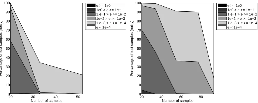
20 30 40 50 0 10 20 30 40 50 60 70 80 90 100
Number of samples
Percantage of test samples (noisy)
e >= 1e0 1e0 > e >= 1e−1 1.e−1 > e >= 1e−2 1e−2 > e >= 1e−3 1.e−3 > e >= 1e−4 e < 1e−4
20 40 60 80
0 10 20 30 40 50 60 70 80 90 100
Number of samples
Percantage of test samples (noisy)
e >= 1e0 1e0 > e >= 1e−1 1.e−1 > e >= 1e−2 1e−2 > e >= 1e−3 1.e−3 > e >= 1e−4 e < 1e−4
Figure 12: KF: Error evolution of the best run (Left: EP=false, Right: EP=true)
1 2 3 4 5 6 7 8 9 101112131415 0 5 10 15 20 25 30 35 40 45
Number of runs
Number of models (S11)
avg: [ 00 45 00 00 ] std: [ 00 00 00 00 ]
Ensemble Rational RBF Kriging
1 2 3 4 5 6 7 8 9 101112131415 0 5 10 15 20 25 30 35 40 45
Number of runs
Number of models (S11)
avg: [ 02 39 02 02 ] std: [ 00 00 00 00 ]
Ensemble Rational RBF Kriging
Figure 13: EE: Composition of the final population (Left: EP=false, Right: EP=true)
10.3 EM Example
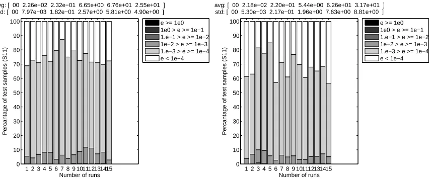
The composition of the final population for each run is shown in Figure 13, and the associated error histogram in Figure 14. The population evolution and corresponding error evolution for the best run are shown in Figures 15 and 16. Table 3 summarizes the results and a plot of the best model can be found in Figure 17. Note that Table 3 shows the cross validation error (CV ) instead of the validation error.
1 2 3 4 5 6 7 8 9 101112131415 0 10 20 30 40 50 60 70 80 90 100
Number of runs
Percantage of test samples (S11)
avg: [ 00 2.26e−02 2.32e−01 6.65e+00 6.76e+01 2.55e+01 ] std: [ 00 7.97e−03 1.82e−01 2.57e+00 5.81e+00 4.90e+00 ]
e >= 1e0 1e0 > e >= 1e−1 1.e−1 > e >= 1e−2 1e−2 > e >= 1e−3 1.e−3 > e >= 1e−4 e < 1e−4
1 2 3 4 5 6 7 8 9 101112131415 0 10 20 30 40 50 60 70 80 90 100
Number of runs
Percantage of test samples (S11)
avg: [ 00 2.18e−02 2.20e−01 5.44e+00 6.26e+01 3.17e+01 ] std: [ 00 5.30e−03 2.17e−01 1.96e+00 7.63e+00 8.81e+00 ]
e >= 1e0 1e0 > e >= 1e−1 1.e−1 > e >= 1e−2 1e−2 > e >= 1e−3 1.e−3 > e >= 1e−4 e < 1e−4
Figure 14: EE: Error histogram of the final best model in each run (Left: EP=false, Right: EP=true)
0 20 40 60 80
0 5 10 15 20 25 30 35 40 45 Generation
Number of models (S11)
Ensemble Rational RBF Kriging
0 10 20 30 40 50 60 0 5 10 15 20 25 30 35 40 Generation
Number of models (S11)
Ensemble Rational RBF Kriging
Figure 15: EE: Population evolution of the best run (Left: EP=false, Right: EP=true)
If we compare the HGA runs with the single model type runs we see significant improvements. Interestingly, the HGA runs need roughly 33-25% less sample evaluations to reach the target accu-racy, and do so in a fraction of the time (less then 8 minutes vs. an average of 43 minutes for the homogeneous runs). Thus here we have a strong case for the use of the HGA.
10.4 LGBB Example
The composition of the final population for each run is shown in Figure 18 and the associated error histogram in Figure 19. The population evolution of the best run is shown in Figure 20. Table 4 shows the comparison with the homogeneous runs. A plot of the response can be found in Figure 21.
100 150 200 0
10 20 30 40 50 60 70 80 90 100
Number of samples
Percantage of test samples (S11)
e >= 1e0 1e0 > e >= 1e−1 1.e−1 > e >= 1e−2 1e−2 > e >= 1e−3 1.e−3 > e >= 1e−4 e < 1e−4
100 150 200 0
10 20 30 40 50 60 70 80 90 100
Number of samples
Percantage of test samples (S11)
e >= 1e0 1e0 > e >= 1e−1 1.e−1 > e >= 1e−2 1e−2 > e >= 1e−3 1.e−3 > e >= 1e−4 e < 1e−4
Figure 16: EE: Error evolution of the best run (Left: EP=false, Right: EP=true)
−1 −0.5
0 0.5
1
−1 −0.5 0 0.5 1 0 0.5 1 1.5
Frequency PostDiameter
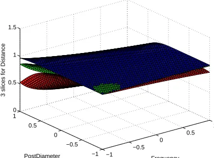
3 slices for Distance
Figure 17: EE: normalized plot of|S11|of the best model overall (HGAEP=true, 3 slices for Distance)
Method |X| σ CVRRSE¯ σ T ERRSE¯ σ time (min)¯ σ
Kriging 7.980E+02 1.137E+02 8.541E-03 7.926E-04 1.881E-02 2.833E-03 7.202E+01 2.780E+01 Rational 8.147E+02 2.314E+02 1.152E-02 4.128E-03 1.708E-02 4.976E-03 4.046E+01 1.914E+01 RBF 6.080E+02 4.226E+01 8.123E-03 6.333E-04 1.556E-02 2.403E-03 1.713E+01 2.159E+00 HGAEP=f alse 1.880E+02 2.536E+01 6.297E-03 1.770E-03 3.518E-02 4.571E-02 7.907E+00 1.440E+00
HGAEP=true 1.980E+02 2.070E+01 6.733E-03 1.457E-03 2.227E-02 1.149E-02 7.722E+00 1.079E+00 Table 3: EE: Comparison with homogeneous evolution