Classifier Cascades and Trees for Minimizing Feature
Evaluation Cost
Zhixiang (Eddie) Xu [email protected]
Matt J. Kusner [email protected]
Kilian Q. Weinberger [email protected]
Department of Computer Science Washington University
1 Brookings Drive
St. Louis, MO 63130, USA
Minmin Chen [email protected]
Olivier Chapelle [email protected]
Criteo
411 High Street
Palo Alto, CA 94301, USA
Editor:Balazs Kegl
Abstract
Machine learning algorithms have successfully entered industry through many real-world
applications (e.g. , search engines and product recommendations). In these applications,
the test-time CPU cost must be budgeted and accounted for. In this paper, we examine
two main components of the test-time CPU cost, classifier evaluation cost and feature
extraction cost, and show how to balance these costs with the classifier accuracy. Since the computation required for feature extraction dominates the test-time cost of a classifier in these settings, we develop two algorithms to efficiently balance the performance with the test-time cost. Our first contribution describes how to construct and optimize a tree of classifiers, through which test inputs traverse along individual paths. Each path extracts different features and is optimized for a specific sub-partition of the input space. Our second contribution is a natural reduction of the tree of classifiers into a cascade. The cascade is particularly useful for class-imbalanced data sets as the majority of instances can be early-exited out of the cascade when the algorithm is sufficiently confident in its prediction. Because both approaches only compute features for inputs that benefit from them the most, we find our trained classifiers lead to high accuracies at a small fraction of the computational cost.
Keywords: budgeted learning, resource efficient machine learning, feature cost sensitive learning, web-search ranking, tree of classifiers
1. Introduction
cascade of classifiers tree of classifiers
4 3
2
1 1
2
3
4
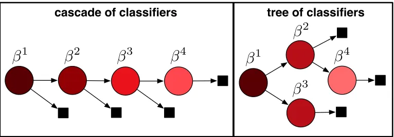
Figure 1: An illustration of two different techniques for learning under a test-time budget. Circular nodes represent classifiers (with parameters β) and black squares pre-dictions. The color of a classifier node indicates the number of inputs passing through it (darker means more). Left: CSCC, a classifier cascade that optimizes the average cost by rejecting easier inputs early. Right: CSTC, a tree that trains expert leaf classifiers specialized on subsets of the input space.
Two main components contribute to the test-time cost. The time required to evaluate a classifier and the time to extract features used by that classifier. Since the features are often heterogeneous, extraction time for different features is highly variable. Imagine introducing a new feature to a product recommendation system that requires 1 second to extract per recommendation. If a web-service provides 100 million recommendations a day (which is not uncommon), it would require 1200 extra CPU days to extract just this feature. While this additional feature may increase the accuracy of the recommendation system, the cost of computing it forevery recommendation is prohibitive. This introduces the problem of balancing the test-time cost and the classifier accuracy. Addressing this trade-off in a principled manner is crucial for the applicability of machine learning.
A key observation for minimizing test-time cost is that not all inputs require the same amount of computation to obtain a confident prediction. One celebrated example is face detection in images, where the majority of all image regions do not contain faces and can often be easily rejected based on the response of a few simple Haar features (Viola and Jones, 2004). A variety of algorithms utilize this insight by constructing a cascade of classifiers (Viola and Jones, 2004; Lefakis and Fleuret, 2010; Saberian and Vasconcelos, 2010; Pujara et al., 2011; Chen et al., 2012; Trapeznikov et al., 2013b). Each stage in the cascade can reject an input or pass it on to a subsequent stage. These algorithms significantly reduce the test-time complexity, particularly when the data is class-imbalanced, and few features
are needed to classify instances into a certain class, as in face detection.
2013a) that is derived based on this observation. CSTC minimizes an approximation of the exact expected test-time cost required to predict an instance. An illustration of a CSTC tree is shown in the right plot of Figure 1. Because the input space is partitioned by the tree, different features are only extracted where they are most beneficial, and therefore, the average test-time cost is reduced. Unlike prior approaches, which reduce the total cost for every input (Efron et al., 2004) or which combine feature cost with mutual information to select features (Dredze et al., 2007), a CSTC tree incorporates input-dependent feature selection into training and dynamically allocates higher feature budgets for infrequently traveled tree-paths.
CSTC incorporates two novelties: 1. it relaxes the expected per-instance test-time cost into a well-behaved optimization; and 2. it is a generalization of cascades to trees. Full trees, however, are not always necessary. In data scenarios with highly skewed class imbalance, cascades might be a better model by rejecting many instances using a small number of features. We therefore apply the same test-time cost derivation to a stage-wise classifier for cascades. The resulting algorithm, Cost-Sensitive Cascade of Classifiers (CSCC), is shown in the left plot of Figure 1. This algorithm supersedes an approach previously proposed,
Cronus (Chen et al., 2012), which is not derived through a formal relaxation of the test-time cost, but performs a clever weighting scheme. We compare and contrast Cronus with CSCC.
Two earlier short papers already introduce CSTC (Xu et al., 2013a) and Cronus (Chen et al., 2012) algorithms, however the present manuscript provides significantly more de-tailed analysis, experimental results and insightful discussion—and it introduces CSCC, which combines insights from all prior work. The paper is organized as follows. Section 2 introduces and defines the test-time cost learning setting. Section 3 presents the tree of clas-sifiers approach, CSTC. In Section 4 we lay out CSCC and relate it to prior work, Cronus, (Chen et al., 2012). Section 5 introduces non-linear extensions to CSTC and CSCC. Sec-tion 6 presents the experimental results on several data sets and discusses the performance differences. Section 7 reviews the prior and related contributions that inspires our work. We conclude in Section 8 by summarizing our contributions and proposing a few future directions.
2. Test-Time Cost
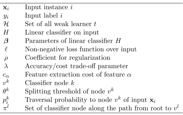
There are several key aspects towards learning under test-time cost budgets that need to be considered: 1. feature extraction cost is relevant and varies significantly across features; 2. features are extracted on-demand rather than prior to evaluation; 3. different features can be extracted for different inputs; 4. the test cost is evaluated in average rather than in absolute (/worst-case) terms (i.e. , several cheap classifications can free up budget for an expensive classification). In this section we focus on learning a single cost-sensitive classifier. We will combine these classifiers to form our tree and cascade algorithms in later sections. We first introduce notation and our general setup, and then provide details on how we address these specific aspects.
Let the data consist of inputs D={x1, . . . ,xn} ⊂ Rd with corresponding class labels
xi Input instance i
yi Input label i
H Set of all weak learnert H Linear classifier on input
β Parameters of linear classifierH ` Non-negative loss function over input
ρ Coefficient for regularization
λ Accuracy/cost trade-off parameter
cα Feature extraction cost of feature α
vk Classifier node k
θk Splitting threshold of node vk
pk
i Traversal probability to nodevk of inputxi
πl Set of classifier node along the path from root to vl
Table 1: Notation used throughout this manuscript.
2.1 Cost-Sensitive Loss Minimization
We learn a classifier H : Rd → Y, parameterized by β, to minimize a continuous, non-negative loss function `overD,
1
nminβ n X
i=1
`(H(xi;β), yi).
We assume that H is a linear classifier, H(x;β) =β>x. To avoid overfitting, we deploy a standardl1 regularization term, |β|to control model complexity. This regularization term has the known side-effect to keep β sparse (Tibshirani, 1996), which requires us to only evaluate a subset of all features. In addition, to balance the test-time cost incurred by the classifier, we also incorporate the cost term c(β) described in the following section. The combined test-time cost-sensitive optimization becomes
min β
X
i
`(x>i β, yi) +ρ|β|
| {z }
regularized loss
+ λ c(β) | {z }
test-cost
, (1)
where λis the accuracy/cost trade-off parameter, and ρ controls the strength of the regu-larization.
2.2 Test-Time Cost
The test-time cost ofH is regulated by the features extracted for that classifier. Different from traditional settings, where all features are computed prior to the application ofH, we assume that features are computedon demand the first time they are used.
We denote the extraction cost for feature α ascα. The cost cα ≥0 is suffered at most once, only for the initial extraction, as feature values can be cached for future use. For a classifier H, parameterized byβ, we can record the features used:
kβαk0 =
1 if featureα is used in H
Here, k · k0 denotes the l0 norm with kak0 = 1 if a6= 0 and kak0 = 0 otherwise. With
this notation, we can formulate the total test-time cost required to evaluate a test inputx
with classifier H (and parameters β) as
c(β) = d X
α=1
cαkβαk0. (3)
The equation (3) can be in any units of cost. For example in medical applications, the feature extraction cost may be in units of “patient agony” or in “examination cost”. The current formulation (1) with cost term (3) still extracts the same features for all inputs and is NP-hard to optimize (Korte and Vygen, 2012, Chapter 15). We will address these issues in the following sections.
3. Cost-Sensitive Tree of Classifiers
We introduce an algorithm that is inspired by the observation that many inputs could be classified correctly based on only a small subset of all features, and this subset may vary across inputs. Our algorithm employs a tree structure to extract particular features for particular inputs, and we refer to it as the Cost-Sensitive Tree of Classifiers (CSTC). We begin by introducing foundational concepts regarding the CSTC tree and derive a global cost term that extends (3) to trees of classifiers and then we relax the resulting loss function into a well-behaved optimization problem.
3.1 CSTC Nodes
The fundamental building block of the CSTC tree is a CSTC node—a linear classifier as described in Section 2.1. Our classifier design is based on the assumption that instances with similar labels tend to have similar features. Thus, we design our tree algorithm to partition the input space based on classifier predictions. Intermediate classifiers determine the path of instances through the tree and leaf classifiers become experts for a small subset of the input space.
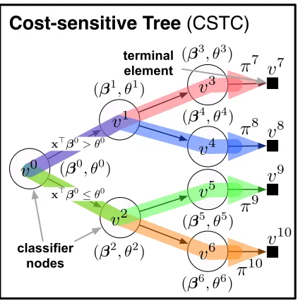
Correspondingly, there are two different nodes in a CSTC tree (depicted in Figure 2):
classifier nodes (white circles) and terminal elements (black squares). Eachclassifier node vk is associated with a weight vectorβk and a threshold θk. These classifier nodes branch inputs by their threshold θk, sending inputs to their upper child if x>
i βk > θk, and to their lower child otherwise. Terminal elements are “dummy” structures and are not real classifiers. They return the predictions of their direct parent classifier nodes—essentially functioning as a placeholder for an exit out of the tree. The tree structure may be a full balanced binary tree of some depth (e.g., Figure 2), or can be pruned based on a validation set. For simplicity, we assume at this point that nodes with terminal element children must be leaf nodes (as depicted in the figure)—an assumption that we will relax later on.
During test-time, inputs traverse through the tree, starting from the root nodev0. The
root node produces predictionsx>i β0and sends the inputxialong one of two different paths, depending on whether x>
classifier nodes
Cost-sensitive Tree
(CSTC)
π
7π
8π
9π
10v
0v
1v
3v
4v
5v
2v
6 terminalelement
v
7v
8v
9v
10 x�β0> θ0x�β0≤θ0
(β1, θ1)
(β0, θ0)
(β2, θ2)
(β3, θ3)
(β4, θ4)
(β5, θ5)
(β6, θ6)
Figure 2: A schematic layout of a CSTC tree. Each node vk is associated with a weight vector βk for prediction and a threshold θk to send instances to different parts of the tree. We solve forβkand θk that best balance the accuracy/cost trade-off for the whole tree. All paths of a CSTC tree are shown in color.
3.2 CSTC Loss
In this section, we discuss the loss and test-time cost of a CSTC tree. We then derive a single global loss function over all nodes in the CSTC tree.
3.2.1 Soft Tree Traversal
As we described before, inputs are partitioned at each node during test-time, and we use a hard threshold to achieve this partitioning. However, modeling a CSTC tree with hard thresholds leads to a combinatorial optimization problem that is NP-hard (Korte and Vygen, 2012, Chapter 15). As a remedy, during training, wesoftly partition the inputs and assign
traversal probabilities p(vk|xi) to denote the likelihood of inputx
i traversing through node
vk. Every inputx
i traverses through the root, so we definep(v0|xi) = 1 for alli. We define a “sigmoidal” soft belief that an inputxi will transition from classifier nodevkwith threshold
θk to its upper child vu as
p(vu|xi, vk) =
1 1 + exp(−(x>
i β k
−θk)). (4)
Let vk be a node with upper child vu and lower childvl. We can express the probabilities of reaching nodes vu and vl recursively as p(vu|xi) = p(vu|x
i, vk)p(vk|xi) and p(vl|xi) =
1−p(vu|x i, vk)
all nodes at tree-depth d, we have
X
v∈Vd
p(v|x) = 1. (5)
In the following paragraphs we incorporate this probabilistic framework into the loss and cost terms of (1) to obtain the corresponding expected tree loss and tree cost.
3.2.2 Expected Tree Loss
To obtain theexpected tree loss, we sum over all nodesV in a CSTC tree and all inputs and weight the loss `(·) of input xi at each node vk by the probability that the input reaches
vk,pk
i =p(vk|xi),
1
n
n X
i=1
X
vk∈V
pki`(x>i βk, yi). (6)
This has two effects: 1. the local loss for each node focuses more on likely inputs; 2. the global objective attributes more weight to classifiers that serve many inputs. Technically, the prediction of the CSTC tree is made entirely by the terminal nodes (i.e. , the leaves), and an obvious suggestion may be to only minimize their classification losses and leave the interior nodes as “gates” without any predictive abilities. However, such a setup creates local minima that send all inputs to the terminal node with the lowest initial error rate. These local minima are hard to escape from and therefore we found it to be important to minimize the loss for all nodes. Effectively, this forces a structure onto the tree that similarly labeled inputs leave through similar leaves and achieves robustness by assigning high loss to such pathological solutions.
3.2.3 Expected Tree Costs
The cost of a test input is the cumulative cost across all classifiers along its path through the CSTC tree. Figure 2 illustrates an example of a CSTC tree with all paths highlighted in color. Every test input must follow along exactly one of the paths from the root to a terminal element. Let L denote the set of all terminal elements (e.g., in Figure 2 we have
L={v7, v8, v9, v10}), and for anyvl∈Lletπl denote the set of allclassifier nodes along the unique path from the rootv0 before terminal elementvl (e.g.,π9={v0, v2, v5}).
For an input x, exiting through terminal node vl, a feature α needs to be extracted if and only if at least one classifier along the pathπluses this feature. We extend the indicator function defined in (2) accordingly:
X
vj∈πl βαj
0
=
1 if featureα is used along path to terminal node vl
0 otherwise. (7)
We can extend the cost term in (3) to capture the traversal cost from root to nodevl as
cl=X α
cα
X
vj∈πl |βαj|
0
Given an input xi, the expected cost is then E[cl|xi] = Pl∈Lp(vl|xi)cl. To approximate the data distribution, we sample uniformly at random from our training set, i.e. , we set
p(xi)≈ 1n, and obtain the unconditional expected cost
E[cost] = n X
i=1 p(xi)
X
l∈L
p(vl|xi)cl≈ X l∈L cl n X i=1
p(vl|xi) 1
n
| {z }
:=pl
=X
l∈L
clpl. (9)
Here, pl denotes the probability that a randomly picked training input exits the CSTC tree through terminal node vl. We can combine (8), (9) with (6) and obtain the objective function,
X
vk∈V
1 n n X i=1 pk
i`ki+ρ|βk| !
| {z }
regularized loss
+λX
vl∈L
pl X α cα X
vj∈πl |βj
α| 0
| {z }
test-time cost
, (10)
where we use the abbreviationspk
i =p(vk|xi) and `ik=`(x>i βk, yi).
3.3 Test-Cost Relaxation
The cost penalties in (10) are exact but difficult to optimize due to the discontinuity and non-differentiability of thel0 norm. As a solution, throughout this paper we use the
mixed-norm relaxation of thel0 norm over sums,
X j X i
|Aij| 0 →X j s X i
(Aij)2, (11)
described by Kowalski (2009). Note that for a vector, this relaxes the l0 norm to the l1
norm,i.e.,P
jkajk0→Pj p
(aj)2=Pj|aj|, recovering the commonly used approximation to encourage sparsity. For matricesA, the mixed norm applies the l1 norm over rows and the l2 norm over columns, thus encouraging a whole row to be all-zero or non-sparse. In
our case this has the natural interpretation to encourage re-use of features that are already extracted along a path. Using the relaxation in (11) on the l0 norm in (10) gives the final optimization problem:
min β0,θ0,...,β|V|,θ|V|
X
vk∈V
1
n
n X
i=1
pki`ki+ρ|βk|
!
| {z }
regularized loss
+λX
vl∈L
pl " X α cα s X
vj∈πl
(βα)j 2
#
| {z }
test-time cost penalty
(12)
We can illustrate the fact that the mixed-norm encourages re-use of features with a simple example. If two classifiers vk 6= vk0 along a path πl use different features with identical weight,i.e.,βk
t ==βk 0
s and t6=s, the test-time cost penalty alongπl is
√
2+√2= 2.
3.4 Optimization
There are many techniques to minimize the objective in (12). We use block coordinate descent, optimizing with respect to the parameters of a single classifier node vk at a time, keeping all other parameters fixed. We perform a level order tree traversal, optimizing each node in order: v1, v2, . . . , v|V|. To minimize (12) (up to a local minimum) with respect to parameters βk, θk we use the lemma below to overcome the non-differentiability of the square-root term (and l1 norm, which we can rewrite as |a| = √a2) resulting from the l0-relaxation (11).
Lemma 1. Given a positive functiong(x), the following holds:
p
g(x) = inf z>0
1 2 "
g(x)
z +z
#
. (13)
It is straight-forward to see thatz=pg(x) minimizes the function on the right hand side and satisfies the equality, which leads to the proof of the lemma.
For each square-root or l1 term we 1) introduce an auxiliary variable (i.e.,z above), 2) substitute in (13), and 3) alternate between minimizing the objective in (12) with respect to
βk, θk and solving for the auxiliary variables. The former minimization is performed with conjugate gradient descent and the latter can be computed efficiently in closed form. This pattern of block-coordinate descent followed by a closed form minimization is repeated until convergence. Note that the objective is guaranteed to converge to a fixed point because each iteration decreases the objective function, which is bounded below by zero. In the following subsection, we detail the block coordinate descent optimization technique. Lemma 1 is only defined for strictly positive functionsg(x). As we are performing function minimization, we can reach cases whereg(x) = 0 and Lemma 1 is ill defined. Thus, as a practical work-around, we clamp values to zero once they are below a small threshold (10−4).
3.4.1 Optimization Details
For reproducibility, we describe the optimization in more detail. Readers not interested in the exact procedure may skip to Section 3.5. As terminal nodes are only placeholders and do not have their own parameters, we only focus on classifier nodes, which are depicted as round circles in Figure 2.
Leaf Nodes. The optimization of leaf nodes (e.g. , v3, v4, v5, v6 in Fig. 2) is simpler
because there are no downstream dependencies. Letvkbe such a classifier node with only a single “dummy” terminal nodevk0
. During optimization of (12), we fix all other parameters
βj, θj of other nodesvj and the respective terms become constants. Therefore, we remove all other paths, and only minimize over the path πk0 from the root to terminal node vk0. Even along the pathπk0
most terms become constant and the only non-constant parameter is βk (the branching parameter θk can be set to −∞ because vk has only one child). We color non-constant terms in the remaining function inblue below,
X
i
pki`(φ(xi)>βk, yi)+ρ|βk|+λ pk0
X
α
cα s
(βk α)2+
X
vj∈πk0\vk
(βjα)2
whereS\bcontain all of the elements inSexceptb. After identifying the non-constant terms, we can apply Lemma 1, making (14) differentiable with respect toβk
α. Let us define auxiliary variablesγα andηαfor 1≤α≤dfor thel1-regularization term and the test-time cost term.
Further, let us collect the constants in the test-time cost termctest-time =Pvj∈πk0\vk(β
j α)2. Applying Lemma 1 results in the following substitutions:
X
α
ρ|βαk|=X α
ρ
q (βk
α)2 −→
X
α
ρ1
2 (βk
α)2 γα
+γα !
,
X
α
cα q
(βk
α)2+ctest-time −→
X
α
cα 1 2
(βk
α)2+ctest-time ηα
+ηα !
. (15)
As a result, we obtain a differentiable objective function after making the above substitu-tions. We can solveβk by alternately minimizing the obtained differentiable function w.r.t.
βk withγα, ηα fixed, and minimizingγα, ηα withβkfixed (i.e., minimizingηα is equivalent to settingηα =
p (βk
α)2+ctest-time ). Recall thatθkdoes not require optimization asvk does
not further branch inputs.
It is straight-forward to show (Boyd and Vandenberghe, 2004, page 72), that the right hand side of Lemma 1 is jointly convex in x and z, so as long as g(x) is a quadratic function of x. Thus, if `(x>i βk, yi) is the squared loss, the substituted objective function is jointly convex inβk and inγα, ηα and therefore we can obtain a globally-optimal solution. Moreover, we can solve βk in closed form. Let us define three design matrices
Xiα= [xi]α, Ωii=pki, Γαα=
ρ γα
+λp
kc α
ηα
,
whereΩand Γare both diagonal and [xi]α is theα feature of instancexi. The closed-form solution for βk is as follows,
βk = (X>ΩX+Γ)−1X>Ωy. (16)
Intermediate Nodes. We further generalize this approach to all classifier nodes. As before, we optimize one node at a time, fixing the parameters of all other nodes. However, optimizing the parametersβk, θk of aninternal nodevk, which has two children affects the parameters of descendant nodes. This affects the optimization of the regularized classifier loss and the test-time cost separately. We state how these terms in the global objective (12) are affected, and then show how to minimize it.
LetS be the set containing all descendant nodes ofvk. Changes to the parametersβk, θk will affect the traversal probabilitiespji for allvj ∈ Sand therefore enter the downstream loss functions. We first state the regularized loss part of (12) and once again color non-constant parameters in blue,
1
n
X
i
pki`(x>i βk, yi) + 1
n
X
vj∈S X
i
pji`(x>i βj, yi) +ρ|βk|. (17)
Algorithm 1 CSTC global optimization
Input: data{xi, yi} ∈ Rd× R, initialized CSTC tree
repeat
fork= 1 toN = # CSTC nodes do repeat
Solve for γ, η (fix βk, θk) using left hand side of (15)
Solve for βk, θk (fixγ, η) with conjugate gradient descent, or in closed-form
until objective changes less thanε end for
until objective changes less than
that passes throughvkand its corresponding probabilitypl. LetP be the terminal elements associated with paths passing through vk. We state the cost function with non-constant parameters in blue,
X
vl∈P pl
X
α
cα v u u t
X
vj∈πl\vk
(βα)j 2+ (βk α)2
!
| {z }
test-time cost
(18)
Adding (17) and (18), with the latter weighted by λ, gives the internal node loss. To make the combined objective function differentiable we apply Lemma 1 to the l1
-regularization, and test-time cost terms and introduce auxiliary variablesγα, ηα as in (15). Similar to the leaf node case, we solve βk, θk by alternately minimizing the new objective w.r.t. βk, θk with γ
α, ηα fixed, and minimizing γα, ηα with fixed βk, θk. Unlike leaf nodes, optimizing the objective function w.r.t. βk, θk cannot be expressed in closed form even with squared loss. Therefore, we optimize it with conjugate gradient descent. Algorithm 1 describes how the entire CSTC tree is optimized.
3.4.2 Node Initialization
The minimization of (12) is non-convex and is therefore initialization dependent. However, minimizing (12) with respect to the parameters of leaf classifiers is convex. We therefore initialize the tree top-to-bottom, starting atv0, and optimizing overβk by minimizing (12) while considering all descendant nodes ofvkas “cut-off” (thus pretending nodevkis a leaf). This initialization is also very fast in the case of a quadratic loss, as it can be solved for in closed form.
3.5 Fine-Tuning
The original test-time cost term in (3) sums over the cost of all features that are extracted during test-time. The relaxation in (11) makes the exactl0cost differentiable and is still well suited to select which features to extract. However, the mixed-norm does also impact the performance of the classifiers, because (different from thel0 norm) larger weights inβincur
0
-0.05
-0.06
2
3 1
0
best potential
node classifier
node
potential node
change in NDCG
iteration
Finish Start
+0.11 +0.02
+0.67
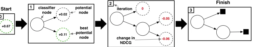
Figure 3: A schematic layout of the greedy tree building algorithm. Each iteration we add the best performing potential node (dashed, above) to the tree. Each potential node is annotated by the improvement in validation-NDCG, obtained with its inclusion (number inside the circle). In this example, after two iterations no more nodes improve the NDCG and the algorithm terminates, converting all remaining potential nodes into terminal elements (black boxes).
, classifiers that make final predictions), while clamping all features with zero-weight to strictly remain zero.
min
¯
βk
X
i
pk i`(x>i β¯
k
, yi) +ρ|β¯ k
|
subject to: ¯βtk= 0 if βtk= 0.
Here, we do not include the cost-term, because the decision regarding which features to use is already made. The final CSTC tree uses these re-optimized weight vectors ¯βk for all leaf classifier nodes vk.
3.6 Determining the Tree Structure
As the CSTC tree does not need to be balanced, its structure is an implicit parameter of the algorithm. We learn and fix the tree structure prior to the optimization and fine-tuning steps in Sections 3.4 and 3.5. We discuss two approaches to determine the structure of the tree in the absence of prior knowledge, the first prunes a balanced tree bottom-up, the second adds nodes top-down, only when necessary. In practice, both techniques produce similar results and we settled on using the pruning technique for all of our experiments.
3.6.1 Tree Pruning
3.6.2 Greedy Tree Building
In contrast to the bottom-up pruning, we can also use a top-down approach to construct the tree structure. Figure 3 illustrates our greedy heuristic for CSTC tree construction. In each iteration, we add the child node that improves the validation criteria (e.g., NDCG) the most on the validation set.
More formally, we distinguish between CSTC classifier nodes and potential nodes. Po-tential nodes (dotted circles in Figure 3) can turn into classifier nodes or terminal elements. Each potential node is initially a trained classifier and annotated with the NDCG value that the CSTC tree would reach on validation with its inclusion. At iteration 0 we learn a single CSTC node by minimizing (12) for the root nodev0, and make it apotential node. At
iteration i >0 we pick the potential node whose inclusion improves the validation NDCG the most (depicted as the dotted green circle) and add it to the tree. Then we create two new potential nodes as its children, and initialize their classifiers by minimizing (12) with all other weight-vectors and thresholds fixed. The splitting thresholdθk is set to move 50% of the validation inputs to the upper child (the thresholds will be re-optimized subsequently). This procedure continues until no more potential nodes improve the validation NDCG, and we convert all remaining potential nodes into terminal elements.
4. Cost-Sensitive Cascade of Classifiers
Many real world applications have data distributions with high class imbalance. One exam-ple is face detection, where the vast majority of all image patches does not contain faces; another example is web-search ranking, where almost all web-pages are irrelevant to a given query. Often, a few features may suffice to detect that an image does not contain a face or that a web-page is irrelevant. Further, in applications such as web-search ranking, the accuracy of bottom ranked instances is irrelevant as long as they are not retrieved at the top (and therefore are not displayed to the end user).
In these settings, the entire focus of the algorithm should be on the most confident positive samples. Sub-trees that lead to only negative predictions, can be pruned effectively as there is no value in providing fine-grained differentiation between negative samples. This further reduces the average feature cost, as negative inputs traverse through shorter paths and require fewer features to be extracted. Previous work obtains these unbalanced trees by explicitly learning cascade structured classifiers (Viola and Jones, 2004; Dundar and Bi, 2007; Lefakis and Fleuret, 2010; Saberian and Vasconcelos, 2010; Chen et al., 2012; Trapeznikov et al., 2013b; Trapeznikov and Saligrama, 2013a). CSTC can incorporate cascades naturally as a special case, in which the tree of classifiers has only a single node per level of depth. However, further modifications can be made to accommodate the specifics of these settings. We introduce two changes to the learning algorithm:
• Inputs of different classes are re-weighted to account for the severe class imbalance.
• Every classifier nodevk has a terminal element as child and is weighted by the prob-ability ofexiting rather than the probability of traversing through nodevk.
Cost-sensitive Cascade (CSCC)
terminal elements early-exit
classifier nodes
v1 v3 v5
v7
terminal element
v2 v4 v6
v0
(β0, θ0) (β2, θ2) (β4, θ4) (β6, θ6)
x�β0
≤θ0 x�β0> θ0
Figure 4: Schematic layout of our classifier cascade with four classifier nodes. All paths are colored in different colors.
weight vectors βk and thresholds θk, C = {(β1, θ1),(β2, θ2),· · · ,(βK,−)}. An input is early-exited from the cascade at node vk ifx>βk< θk and is sent to its terminal element
vk+1. Otherwise, the input is sent to the next classifier node. At the final node vK a prediction is made for all remaining inputs via x>βK.
In CSTC, most classifier nodes are internal and branch inputs. As such, the predictions need to be similarly accurate for all inputs to ensure that they are passed on to the correct part of the tree. In CSCC, each classifier node early-exits a fraction of its inputs, providing theirfinal prediction. As mistakes of such exiting inputs are irreversible, the classifier needs to ensure particularly low error rates for this fraction of inputs. All other inputs are passed down the chain to later nodes. This key insight inspires us to modify the loss function of CSCC from the original CSTC formulation in (6). Instead of weighting the contribution of classifier loss`(x>i βk, yi) by pk
i, the probability of input xi traversing through node vk, we weight it withpki+1, the probability of exiting through terminal nodevk+1. As a second
modification, we introduce an optional class-weight wyi > 0 which absorbs some of the
impact of the class imbalance. The resulting loss becomes:
1
n
n X
i=1
X
vk∈V
wyip
k+1
i `(x >
i βk, yi).
The cost term is unchanged and the combined cost-sensitive loss function of CSCC becomes
X
vk∈V
1
n
n X
i=1 wyip
k+1
i `
k i
!
+ρ|βk|
| {z }
regularized loss
+λX
vl∈L
pl
d X
α=1 cα
s X
vj∈πl
(βα)j 2
| {z }
feature cost penalty
. (19)
4.1 Cronus
CSCC supersedes previous work on cost sensitive learning of cascades by the same authors, Chen et al. (2012). The previous algorithm, named Cronus, shares the same loss terms as CSCC, however the feature and evaluation cost of each node is weighted by the expected number of inputs, pk,within the mixed-norm (highlighted in color):
X
vk∈V
1
n
n X
i=1 wyip
k+1
i `ki !
+ρ|βk|
| {z }
regularized loss
+λ
d X
α=1 cα
s X
vk∈V
(pkβk α)2
| {z }
feature cost penalty .
In contrast, CSCC in (19) sums over the weighted cost of all exit paths. The two formu-lations are similar, but CSCC may be considered more principled as it is derived from the exact expected cost of the cascade. As we show in Section 6, this does translate into better empirical accuracy/cost trade-offs.
5. Extension to Non-Linear Classifiers
Although CSTC’s decision boundary may be non-linear, each individual node classifier is linear. For many problems this may be too restrictive and insufficient to divide the input space effectively. In order to allow non-linear decision boundaries we map the input into a more expressive feature space with the “boosting trick” (Friedman, 2001; Chapelle et al., 2011), prior to our optimization. In particular, we first train gradient boosted regression trees with a squared loss penalty forT iterations and obtain a classifierH0(x
i) =PTt=1ht(xi), where each function ht(·) is a limited-depth CART tree (Breiman, 1984). We then define the mapping φ(xi) = [h1(xi), . . . , hT(xi)]> and apply it to all inputs. The boosting trick is particularly well suited for our feature cost sensitive setting, as each CART tree only uses a small number of features. Nevertheless, this pre-processing step does affect the loss function in two ways: 1. the feature extraction now happens within the CART trees; and 2. the evaluation time of the CART trees needs to be taken into account.
5.1 Feature Cost After the Boosting Trick
After the transformation xi→φ(xi), each input is T−dimensional and consequently, we have the weight vectors β ∈ RT. To incorporate the feature extraction cost into our loss, we define an auxiliary matrix F∈ {0,1}d×T with F
αt= 1 if and only if the CART tree ht uses feature fα. With this notation, we can incorporate the CART-trees into the original feature extraction cost term for a weight vector β, as stated in (3). The new formulation and its relaxed version, following the mixed-norm relaxation as stated in (11), are then:
d X
α=1 cα
T X
t=1
|Fαtβt|
0
−→
d X
α=1 cα
v u u t
T X
t=1
(Fαtβt)2.
adapt the feature extraction cost of the path through a CSTC tree, originally defined in (8), which becomes:
d X α=1 cα X
vj∈πl
T X
t=1
|Fαtβtj| 0 −→ d X α=1 cα v u u t X
vj∈πl
T X
t=1
(Fαtβtj)2. (20)
5.2 CART Evaluation Cost
The evaluation of a CART tree may be non-trivial or comparable to the cost of feature extraction and its cost must be accounted for. We define a constantet≥0, which captures the cost of the evaluation of the tth CART tree. We can express this evaluation cost for a single classifier with weight vector β in terms of thel0 norm and again apply the mixed norm relaxation (11). The exact (left term) and relaxed evaluation cost penalty (right term) can be stated as follows:
T X
t=1
etkβtk0−→
T X
t=1 et|βt|
The left term incurs a cost of et for each tree ht if and only if it is assigned a non-zero weight by the classifier,i.e.,βt6= 0. Similar to feature values, we assume that CART tree evaluations can be cached and only incur a cost once (the first time they are computed). With this assumption, we can express the exact and relaxed CART evaluation cost along a pathπl in a CSTC tree as
T X t=1 et X
vj∈πl |βtj|
0 −→ T X t=1 et s X
vj∈πl
(βtj)2. (21)
It is worth pointing out, that (21) is analogous to the feature extraction cost with linear classifiers (8) and its relaxation, as stated in (12).
5.3 CSTC and CSCC with Non-Linear Classifiers
We can integrate the two CART tree aware cost terms (20) and (21) into the optimization problem in (12). The final objective of the CSTC tree after the “boosting trick” becomes then
X
vk∈V
1
n
n X
i=1
pki`ki+ρ|βk| !
| {z }
regularized loss
+λX
vl∈L
pl " X t et s X
vj∈πl
(βtj)2
| {z }
CART evaluation cost penalty
+ d X α=1 cα v u u t X
vj∈πl
T X
t=1
(Fαtβtj)2
| {z }
feature cost penalty
#
. (22)
The objective in (22) can be optimized with the same block coordinate descent algorithm, as described in Section 3.4. Similarly, the CSCC loss function with non-linear classifiers becomes
X
vk∈V
1
n
n X
i=1 wyip
k+1
i `
k i
!
+ρ|βk|
| {z }
regularized loss
+λX
vl∈L
pl " X t et s X
vj∈πl
(βjt)2
| {z }
evaluation cost + d X α=1 cα v u u t X
vj∈πl
T X
t=1
(Fαtβtj)2
| {z }
feature cost
#
In the same way, Cronus may be adapted for non-linear classification (see: Chen et al., 2012). To avoid over-fitting, we use validation set to perform early-stopping during optimizing objective function 22.
6. Results
In this section, we evaluate CSTC on a synthetic cost-sensitive learning task and compare it with competing algorithms on two large-scale, real world benchmark problems. Addi-tionally, we discuss the differences between our models for several learning settings. We provide further insight by analyzing the features extracted on a these data sets and looking at how CSTC tree partitions the input space. We judge the effect of the cost-sensitive regularization by looking at how removing terms and varying parameters affects CSTC on real world data sets. We also present detailed results of CSTC on a cost-sensitive version of the MNIST data set, demonstrating that it extracts intelligentper-instance features. We end by proposing a criterion that is designed to judge if CSTC will perform well on a data set.
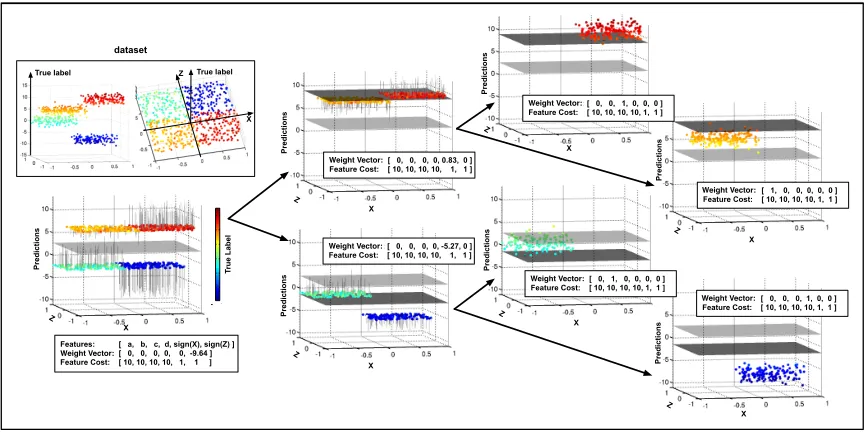
6.1 Synthetic Data
We construct a synthetic regression data set consisting of points sampled from the four quadrants of the X, Z-plane, whereX=Z∈[−1,1]. The features belong to two categories: cheap features: sign(x), sign(z) with costc= 1, which can be used to identify the quadrant of an input; and expensive features: z++, z+−, z−+, z−− with cost c= 10, which equal the exact label of an input if it is from the corresponding quadrant (or a random number otherwise). Since in this synthetic data set we do not transform the feature space, we have
φ(x) =x, and F (the weak learner feature-usage variable) is the 6×6 identity matrix. By design, a perfect classifier can use the two cheap features to identify the sub-region of an instance and then extract the correct expensive feature to make a perfect prediction. The minimum feature cost of such a perfect classifier is exactlyc= 12 per instance. We construct the data set to be a regression problem, with labels sampled from Gaussian distributions with quadrant-specific means µ++, µ−+, µ+−, µ−− and variance 1. The individual values for the label means are picked to satisfy the CSTC assumption,i.e., that the prediction of similar labels requires similar features. In particular, as can be seen in Figure 5 (top left), label means from quadrants with negativez−coordinates (µ+−, µ−−) are higher than those with positive z−coordinates (µ++, µ−+).
Pr ed ic ti o n s Pr ed ic ti o n s Pr ed ic ti o n s Pr ed ic ti o n s Pr ed ic ti o n s Pr ed ic ti o n s Pr ed ic ti o n s Tr u e L ab el X X X X Z Z Z Z
Feature Vector: [ 0, 0, 0, 0, -5.27, 0 ] Feature Cost: [ 10, 10, 10, 10, 1, 1 ]
Features: [ a, b, c, d, sign(X), sign(Z) ] Feature Vector: [ 0, 0, 0, 0, 0, -9.64 ] Feature Cost: [ 10, 10, 10, 10, 1, 1 ]
Feature Vector: [ 0, 0, 0, 0, 0.83, 0 ] Feature Cost: [ 10, 10, 10, 10, 1, 1 ]
Feature Vector: [ 0, 0, 1, 0, 0, 0 ] Feature Cost: [ 10, 10, 10, 10, 1, 1 ]
Feature Vector: [ 1, 0, 0, 0, 0, 0 ] Feature Cost: [ 10, 10, 10, 10, 1, 1 ]
Feature Vector: [ 0, 1, 0, 0, 0, 0 ] Feature Cost: [ 10, 10, 10, 10, 1, 1 ]
Feature Vector: [ 0, 0, 0, 1, 0, 0 ] Feature Cost: [ 10, 10, 10, 10, 1, 1 ] X
Z True label True label dataset X Z X Z X Z Weight Vector: Weight Vector: Weight Vector: Weight Vector: Weight Vector: Weight Vector: Weight Vector:
Figure 5: CSTC on synthetic data. The box at left describes the data set. The rest of the figure shows the trained CSTC tree. At each node we show a plot of the predictions made by that classifier and the feature weight vector. The tree obtains a perfect (0%) test-error at the optimal cost of 12 units.
6.2 Yahoo! Learning to Rank
To evaluate the performance of CSTC on real-world tasks, we test it on the Yahoo! Learning to Rank Challenge (LTR) data set. The set contains 19,944 queries and 473,134 documents. Each query-document pair xi consists of 519 features. An extraction cost, which takes on a value in the set {1,5,20,50,100,150,200}, is associated with each feature.1 The unit of
these values turns out to be approximately the number of weak learner evaluations ht(·) that can be performed while the feature is being extracted. The label yi ∈ {4,3,2,1,0} denotes the relevancy of a document to its corresponding query, with 4 indicating a perfect match. We measure the performance using normalized discounted cumulative gain at the 5th position (NDCG@5) (J¨arvelin and Kek¨al¨ainen, 2002), a preferred ranking metric when multiple levels of relevance are available. Letπ be an ordering of all inputs associated with a particular query (π(r) is the index of the rth ranked document and y
π(r) is its relevance
label), then the NDCG ofπ at position P is defined as
N DCG@P(π) = DCG@P(π)
DCG@P(π∗) withDCG@P(π) = P X
r=1
2yπ(r) −1 log2(r+ 1),
whereπ∗is an optimal ranking (i.e., documents are sorted in decreasing order of relevance). To introduce non-linearity, we transform the input features into a non-linear feature space
x → φ(x) with the boosting trick (see Section 5) with T = 3000 iterations of gradient boosting and CART trees of maximum depth 4. Unless otherwise stated, we determine the CSTC depth by validation performance (with a maximum depth of 10).
0 0.5 1 1.5 2
x 104
0.705 0.71 0.715 0.72 0.725 0.73 0.735 0.74
Stage−wise regression (Friedman, 2001)
Single cost−sensitive classifier
Early exit s=0.2 (Cambazoglu et. al. 2010) Early exit s=0.3 (Cambazoglu et. al. 2010) Early exit s=0.5 (Cambazoglu et. al. 2010) Cronus optimized (Chen et. al. 2012)
CSTC w/o fine−tuning
CSTC
NDCG @ 5
Cost 104
Figure 6: The test ranking accuracy (NDCG@5) and cost of various cost-sensitive classifiers. CSTC maintains its high retrieval accuracy significantly longer as the cost-budget is reduced.
Figure 6 shows a comparison of CSTC with several recent algorithms for test-time budgeted learning. We show NDCG versus cost (in units of weak learner evaluations). We obtain the curves of CSTC by varying the accuracy/cost trade-off parameterλ(and perform early stopping based on the validation data, for fine-tuning). For CSTC we evaluate eight settings, λ={1
3, 1
2,1,2,3,4,5,6}. In the case of stage-wise regression, which is not
cost-sensitive, the curve is simply a function of boosting iterations. We include CSTC with and without fine-tuning. The comparison shows that there is a small but consistent benefit to fine-tuning the weights as described in Section 3.5.
For competing algorithms, we include Early exit (Cambazoglu et al., 2010) which im-proves upon stage-wise regression by short-circuiting the evaluation of unpromising docu-ments at test-time, reducing the overall test-time cost. The authors propose several criteria for rejecting inputs early and we use the best-performing method “early exits using proxim-ity threshold”, where at theithearly-exit, we remove all test-inputs that have a score that is at least 300−i
299 slower than the fifth best input, andsdetermines the power of the early-exit.
The single cost-sensitive classifier is a trivial CSTC tree consisting of only the root node
Pre
ci
si
o
n
@
5
0 0.5 1 1.5 2
x 104 0.095
0.1 0.105 0.11 0.115 0.12 0.125 0.13 0.135 0.14
Stageïwise regression (Friedman, 2001) Early exit s=0.2 (Cambazoglu et. al. 2010) Early exit s=0.3 (Cambazoglu et. al. 2010) Early exit s=0.3 (Cambazoglu et. al. 2010) AdaBoostRS_AC (Reyzin, 2011) ANDïOR (Dundar and Bi, 2007) Cronus (Chen et. al 2012)
CSTC CSCC
Cost
0.145
Figure 7: The test ranking accuracy (Precision@5) and cost of various budgeted cascade classifiers on the Skew-LTR data set with high class imbalance. CSCC outper-forms similar techniques, requiring less cost to achieve the same performance.
as the cost-budget is reduced. It is interesting to observe that the single cost-sensitive clas-sifier outperforms stage-wise regression (due to the cost sensitive regularization) but obtains much worse cost/accuracy trade offs than the full CSTC tree. This demonstrates that the tree structure is indeed an important part of the high cost effectiveness of CSTC.
6.3 Yahoo! Learning to Rank: Skewed, Binary
To evaluate the performance of our cascade approach CSCC, we construct a highly class-skewed binary data set using the Yahoo! LTR data set. We define inputs having labels
yi ≥ 3 as ‘relevant’ and label the rest as ‘irrelevant’, binarizing the data in this way. We also replicate each negative, irrelevant example 10 times to simulate the scenario where only a few documents are highly relevant, out of many candidate documents. After these modifications, the inputs have one of two labels {−1,1}, and the ratio of +1 to −1 is 1/100. We call this data set LTR-Skewed. This simulates an important setting, as in many time-sensitive real life applications the class distributions are often very skewed.
For the binary case, we use the ranking metric Precision@5 (the fraction of top 5 doc-uments retrieved that are relevant to a query). It best reflects the capability of a classifier to precisely retrieve a small number of relevant instances within a large set of irrelevant documents. Figure 7 compares CSCC and Cronus with several recent algorithms for binary budgeted learning. We show Precision@5 versus cost (in units of weak learner evaluations). Similar to CSTC, we obtain the curves of CSCC by varying the accuracy/cost trade-off parameterλ. For CSCC we evaluate eight settings,λ={1
3, 1
2,1,2,3,4,5,6}.
cas-1 2 3 4 5 6 7 8 9 10 0
0.2 0.4 0.6 0.8 1
Depth
Feature Used
c=1 (123) c=5 (31) c=20 (191) c=50 (125) c=100 (16) c=150 (32) c=200 (1)
Tree Depth Cost
1 2 3 4
0 0.2 0.4 0.6 0.8 1
Depth
Feature Used
Yahoo Learning To Rank
Cronus cascade CSTC tree
v0 v1
v2 v3
v4
v5
v6 v7
v9
v11
v13
v14 v29 CSTC pruned tree structure
cascade nodes tree depth
Pro
po
rt
io
n
of
F
ea
tu
re
s
Pro
po
rt
io
n
of
F
ea
tu
re
s
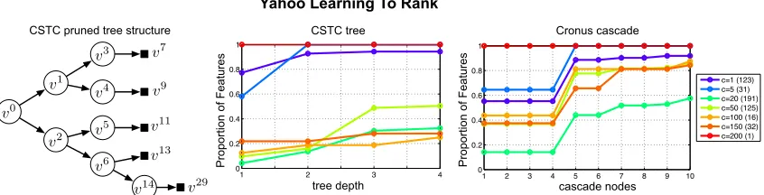
Figure 8: Left: The pruned CSTC tree, trained on the Yahoo! LTR data set. The ratio of features, grouped by cost, are shown for CSTC (center) and Cronus (right). The number of features in each cost group is indicated in parentheses in the legend. More expensive features (c≥20) are gradually extracted deeper in the structure of each algorithm.
cade of classifiers and employ anAND-ORscheme with the loss function that treats negative inputs and positive inputs separately. This setup is based on the insight that positive in-puts are carried all the way through the cascade (i.e. , each classifier must classify them as positive), whereas negative inputs can be rejected at any time (i.e. , it is sufficient if a single classifier classifies them as negative). The loss for positive inputs is the maximum loss across all stages, which corresponds to the AND operation, and encourages all classi-fiers to make correct predictions. For negative inputs the loss is the minimum loss of all classifiers, which corresponds to the OR operation, and which enforces that at least one classifier makes a correct prediction. Different from our approach, their algorithm requires pre-assigning features to each node. We therefore use five nodes in total, assigning fea-tures of cost ≤5,≤20,≤50,≤150,≤200. The curve is generated by varying a loss/cost trade-off parameter (similar to λ). Finally, we also compare with the cost sensitive ver-sion of AdaboostRS (Reyzin, 2011). This algorithm resamples deciver-sion trees, learned with AdaBoost (Freund et al., 1999), inversely proportional to a tree’s feature cost. As this algo-rithm involves random sampling, we averaged over 10 runs and show the standard deviations in both precision and cost.
Yahoo Learning To Rank, Skewed Binary
1 2 3 4 5 6 7 8 9 10 0 0.2 0.4 0.6 0.8 1 Depth Feature Used
1 2 3 4 5 6 7 8 9 10 0 0.2 0.4 0.6 0.8 1 Depth Feature Used c=1 (123) c=5 (31) c=20 (191) c=50 (125) c=100 (16) c=150 (32) c=200 (1) Pro po rt io n of F ea tu re s
1 2 3 4 5 6
0 0.2 0.4 0.6 0.8 1 Depth Feature Used Pro po rt io n of F ea tu re s Cronus cascade AND-OR cascade
AND-OR nodes Cronus nodes
1 2 3 4 5 6 7 8 9 10 0 0.2 0.4 0.6 0.8 1 Depth Feature Used
1 2 3 4 5 6 7 8 9 10 0 0.2 0.4 0.6 0.8 1 Depth Feature Used CSCC Pro po rt io n of F ea tu re s CSCC nodes
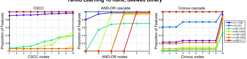
Figure 9: The ratio of features, grouped by cost, that are extracted at different depths of CSCC (left), AND-OR (center) and Cronus (right). The number of features in each cost group is indicated in parentheses in the legend.
6.4 Feature Extraction
Based on the LTR and LTR-Skewed data sets, we investigate the features extracted by various algorithms in each scenario. We fist show the features retrieved in the regular balanced class data set (LTR). Figure 8 (left) shows the pruned CSTC tree learned on the LTR data set. The plot in the center demonstrates the fraction of features, with a particular cost, extracted at different depths of the CSTC tree. The rightmost plot shows the features extracted at different nodes of Cronus. We observe a general trend that for both CSTC and Cronus, as depth increases, more features are being used. However, cheap features (c≤5) are all extracted early-on, whereas expensive features (c≥ 20) are extracted by classifiers sitting deeper in the tree. Here, individual classifiers only cope with a small subset of inputs and the expensive features are used to classify these subsets more precisely. The only feature that has cost 200 is extracted at all depths—which seems essential to obtain high NDCG (Chen et al., 2012). Although Cronus has larger depth than CSTC (10 vs 4), most nodes in Cronus are basically dummy nodes (as can be seen by the flat parts of the feature usage curve). For these nodes all weights are zeros, and the threshold is a very small negative number, allowing all inputs to pass through.
Predictive Node Classifier Similarity
1.00 0.85
1.00
1.00
1.00 0.85
0.81
0.81 0.76
0.76
0.90
0.90
0.83
0.83
0.88
0.88
0.64
0.72
0.75
0.84
0.72 0.75 0.84 1.00 0.64
v
3
v
4
v
5
v
6
v6 v5 v4 v3
v
14
v14
v0
v1
v3
1.23
1.67
0.56
0.36 0.84
2.02
1.39
v7
v9
v13
v29 v5
1.13
v11
CSTC Tree
v2
v4
v6
v14
Figure 10: (Left) The pruned CSTC-tree generated from the Yahoo! Learning to Rank data set. (Right) Jaccard similarity coefficient between classifiers within the learned CSTC tree.
one of the reasons that CSCC and Cronus achieve better performance over existing cascade algorithms.
6.5 Input Space Partition
CSTC has the ability to split the input space and learn more specialized classifiers sitting deeper in the tree. Figure 10 (left) shows a pruned CSTC tree (λ= 4) for the LTR data set. The number above each node indicates the average label of the testing inputs passing through that node. We can observe that different branches aim at different parts of the input domain. In general, the upper branches focus on correctly classifying higher-ranked documents, while the lower branches target low-rank documents. Figure 10 (right) shows the Jaccard matrix of the leaf classifiers (v3, v4, v5, v6, v14) from this CSTC tree. The number
in field i, j indicates the fraction of shared features between vi and vj. The matrix shows a clear trend that the Jaccard coefficients decrease monotonically away from the diagonal. This indicates that classifiers share fewer features in common if their average labels are further apart—the most different classifiers v3 and v14 have only 64% of their features
6.6 CSTC Sensitivity
Recall the CSTC objective function with non-linear classifiers,
X
vk∈V
1
n
n X
i=1
pki`ki+ρ|βk|
!
| {z }
regularized loss
+λX
vl∈L
pl " X t et s X
vj∈πl
(βtj)2
| {z }
CART evaluation cost penalty
+ d X α=1 cα v u u t X
vj∈πl
T X
t=1
(Fαtβtj)2
| {z }
feature cost penalty
#
.
In order to judge the effect of different terms in the cost-sensitive regularization we ex-periment with removing the CART evaluation cost penalty (or simply ‘evaluation cost’) and/or the feature cost penalty. Figure 11 (Left) shows the performance of CSTC and the less cost-sensitive variants, after removing one or both of the penalty terms, on the Yahoo! LTR data set. As we suspected, the feature cost term seems to contribute most to the performance of CSTC. Indeed, only taking into account evaluation cost severely impairs the model. Without considering cost, CSTC seems to overfit even though the remaining
l1-regularization prevents the model from extracting all possible features.
0 2000 4000 6000 8000 10000 0.705 0.71 0.715 0.72 0.725 0.73 0.735 0.74 CSTC
CSTC with different l
Cost
NDCG @ 5
0 2000 4000 6000 8000 10000
0.705 0.71 0.715 0.72 0.725 0.73 0.735 0.74
CSTC varying h (l found by CV)
CSTC varying l (h = 1)
0 0.5 1 1.5 2
x 104 0.705 0.71 0.715 0.72 0.725 0.73 0.735 0.74 CSTC
feature cost only evaluation cost only no cost
Cost
NDCG @ 5
0 2000 4000 6000 8000 10000
0.705 0.71 0.715 0.72 0.725 0.73 0.735 0.74
CSTC varying h (l found by CV)
CSTC varying l (h = 1)
0.2 0.4 0.6 0.8 1
x 104 0
Figure 11: Two plots showing the sensitivity of CSTC to different cost regularization and hyperparameters. Left: The test ranking accuracy (NDCG@5) and cost of differ-ent CSTC cost-sensitive variants. Right: The performance of CSTC for different values of hyperparameterρ∈[0.5,0.6,0.7,0.8,0.9,1,2,3,4,5].
We are also interested in judging the effect of the l1-regularization hyperparameter ρ on the performance of CSTC. Figure 11 (Right) shows for λ = 1 different settings of
ρ∈[0.5,0.6,0.7,0.8,0.9,1,2,3,4,5] and the resulting change in cost and NDCG. The result shows that varying ρ does follow the CSTC NDCG/cost trade-off for a little bit, however ultimately leads to a reduction in accuracy. This supports our hypothesis that the cost term is crucial to obtain low cost classifiers.
6.7 Cost-Sensitive MNIST
0 50 100 150 200 250 300 350 400 450 0.03
0.04 0.05 0.06 0.07 0.08 0.09 0.1 0.11 0.12
CSTC
λ1= 1−1
λ4= 1−2
λ7= 1−3 λ3= 3×1−2
Cost
Erro
r
Figure 12: The test error vs. cost trade-off for CSTC on the cost-sensitive MNIST data set
original size), and concatenated all features, resulting in d = 1120 features. We assigned each feature a costc= 1. To obtain a baseline error rate for the data set we trained a support vector machine (SVM) with a radial basis function (RBF) kernel. To select hyperparameters
C (SVM cost) and γ (kernel width) we used 100 rounds of Bayesian optimization on a validation set (we found C = 753.1768, γ = 0.0198). An RBF-SVM trained with these hyperparameters achieves a test error of 0.005 for cost c = 1120. Figure 12 shows error versus cost for different values of the trade-off parameter λ. We note that CSTC smoothly trades off feature cost for error, quickly reducing error initially at small increases in cost.
Figure 13 shows the features extracted and trees built for different values of λ for the cost-sensitive MNIST data set. For each value, we show the paths of one randomly selected 3-instance (lower paths) and one 8-instance (upper paths). For each node in each path we show the features extracted at each of the four resolutions in boxes (red indicates a feature was not extracted). In general, asλis decreased, more features are extracted. Additionally, for a single λ, nodes along a path tend to use the same features. Finally, even when the algorithm is restricted to use very little cost (i.e., theλ1 tree) it is still able to find features that distinguish the classes in the data set, sending the 3 and 8-instances along different paths in the tree.
6.8 CSTC Criterion
CSTC implicitly assumes that similarly-labeled inputs can be classified using similar features by sending instances with different predictions to different classifiers. Since not all data sets have such a property, we propose a simple test which indicates if a data set satisfies this assumption. We train binary classifiers withl1-regularization for neighboring pairs of labels.
v0
v1
v3
v4
v5
v2
v6
v1
v3
v4
v5
v6
v2
v0
v0
v1
v3
v2
v4
v10
v0
v1
v3
v2
v4
v9
v10
v9
λ7= 1−3
λ4 = 1−2
λ3= 3×1−2
λ1 = 1−1
Figure 13: Trees generated for differentλon the cost-sensitive MNIST data set. For eachλ
we show the path of one 3-instance (orange or green) and one 8-instance (red). For each node these instances visit, we show the features extracted above (for the 8-instance) and below (for the 3-instance) the trees in boxes for different resolutions (red indicates a feature was not extracted).
Jaccard coefficients decrease monotonically away from the diagonal. This indicates that classifiers share fewer features in common if the average label of their training data sets are further apart—a good indication that on this data set CSTC will perform well.
7. Related Work
In the following we review different methods for budgeting the computational cost during test-time starting with simply reducing the feature space vial1-regularization up to recent
work in budgeted learning.
7.1 l1 Norm Regularization
A related approach to control test-time cost is feature selection with l1 norm regulariza-tion (Efron et al., 2004),
min
β `(H(x;β),y) +λ|β|,
Classifier
C
la
ssi
fie
r
class 0 & 1 class 1 & 2 class 2 & 3 class 3 & 4
cl
ass
0
&
1
cl
ass
1
&
2
cl
ass
2
&
3
cl
ass
3
&
4
1.00 0.49
1.00
1.00
1.00 0.49
0.41
0.41 0.32
0.32
0.52
0.52
0.33
0.33
0.49
0.49
Figure 14: Jaccard similarity coefficient between binary classifiers learned on the LTR data set. The binary classifiers are trained withl1-regularization for neighboring pairs
of labels. As an example, the LTR data set contains five labels{0,1,2,3,4}, four binary classifiers are trained, (0vs.1, 1 vs.2, etc.). There is a clear trend that the Jaccard coefficients decrease monotonically away from the diagonal. This indicates that classifiers share fewer features in common if the average label of their training data sets are further apart—an indication that CSTC will perform well.
approach is that it extracts a feature forall inputs ornone, which makes it uncompetitive with more flexible cascade or tree models.
7.2 Feature Selection
Another approach, extending l1-regularization, is to select features using some external
criterion that naturally limits the number of features used. Cesa-Bianchi et al. (2011) construct a linear classifier given a budget by selecting one instance at a time, then using the current parameters to select a useful feature. This process is repeated until the budget is met. Globerson and Roweis (2006) formulate feature selection as an adversarial game and use minimax to develop a worst-case strategy, assuming feature removal at test-time. These approaches, however, are unaware of the test-time cost in (3), and fail to pick the optimal feature set that best trades-off loss and cost. Dredze et al. (2007) gets closer to directly balancing this trade-off by combining the cost to select a feature with the mutual information of that feature to build a decision tree that reduces the feature extraction cost. This work, though, does not directly minimize the total test-time cost vs. accuracy trade-off of the classifier. Most recently, Xu et al. (2013b) proposed to learn a new feature representation entirely using selected features.
7.3 Linear Cascades