Universal Consistency of Localized Versions
of Regularized Kernel Methods
Robert Hable [email protected]
Department of Mathematics University of Bayreuth D-95440 Bayreuth, Germany
Editor:G´abor Lugosi
Abstract
In supervised learning problems, global and local learning algorithms are used. In contrast to global learning algorithms, the prediction of a local learning algorithm in a testing point is only based on training data which are close to the testing point. Every global algorithm such as support vector machines (SVM) can be localized in the following way: in every testing point, the (global) learning algorithm is not applied to the whole training data but only to theknearest neighbors (kNN) of the testing point. In case of support vector machines, the success of such mixtures of SVM and kNN (called SVM-KNN) has been shown in extensive simulation studies and also for real data sets but only little has been known on theoretical properties so far. In the present article, it is shown how a large class of regularized kernel methods (including SVM) can be localized in order to get a universally consistent learning algorithm.
Keywords: machine learning, regularized kernel methods, localization, SVM, k-nearest neigh-bors, SVM-KNN
1. Introduction
In a supervised learning problem, the goal is to predict the valuey of an unobserved output vari-ableY after observing the valuex of an input variableX. A predictor is a function f which maps the observed input valuex (called testing data point) to a prediction f(x)of the unobserved out-put value y. Choosing a predictor f = fDn is done on base of previously observed data Dn=
(x1,y1), . . . ,(xn,yn)
(called trainig data). A learning algorithm is a function Dn7→ fDn which
maps training dataDn to a predictor fDn. Among the learning algorithms commonly used in
ma-chine learning, there are local and global algorithms. The most prominent example of a local algo-rithm isk-nearest neighbors(kNN). In case of a local algorithmDn7→ fDn, the prediction fDn(x)in
a testing data pointxis not based on the whole training data but only on those training data points
(xi,yi) which are close tox. In case of a global algorithm, choosing a predictor fDn is based on a
global criterion—such as (penalized) empirical risk minimization—and, accordingly, the prediction fDn(x)in a pointxcan also be based on training data points(xi,yi)which are not close tox.
Typi-cal examples of global algorithms are regularized kernel methods such assupport vector machines (SVM).
func-tion. This is a problem for global algorithms because the complexity of the selected predictor fDn
is usually regularized by one or several hyperparameters which are fixed for the whole input space. One way to overcome this problem is to separate the input space into several parts in a first step and to separately use a global algorithm for each of the separated parts. For example, the input space is separated by use of decision trees and then SVMs are separately applied on the separated parts of the input space; see, for example, Bennett and Blue (1998), Wu et al. (1999), and Chang et al. (2010). Another possibility is to “localize” a global algorithm. This can be done in the following way: (1) select a few training data points which are close to the testing data point, (2) determine a predictor based on the selected training data points by use of a (global) learning algorithm, and (3) calculate the prediction in the testing data point. A number of algorithms which have been sug-gested in the literature can be described in this way. These algorithms only differ in the way how data points are selected in (1) and which learning algorithm is used in (2). An early investigation of such methods is Bottou and Vapnik (1992) and Vapnik and Bottou (1993). A number of recent articles apply such an approach to support vector machines (SVM). That is, SVM is used in (2), but there are differences in (1): In Zhang et al. (2006), data points are selected in the same way as for kNN. That is, the prediction in a testing pointxis given by that SVM which is calculated based on thekn training points which are nearest to x; the natural number kn acts as a hyperparameter.
In order to decide which training points are thekn closest ones to x, a metric on the input space
is needed. Zhang et al. (2006) considers different metrics. As this approach is a mixture between kNN and SVM, it is called SVM-KNN. Independently, a similar approach has been developed by E. Blanzieri and others. The main difference to Zhang et al. (2006) is that distances (for select-ing thekn nearest neighbors) are not measured in the input space but in the feature space (i.e., in
the RKHS associated with the kernel of the SVM). This approach has been extensively studied in experimental comparisons in Blanzieri and Bryl (2007a), Blanzieri and Bryl (2007b), Segata and Blanzieri (2009) and Blanzieri and Melgani (2008) where the latter publication also derives a local bound on the generalization error. Another slightly different approach is developed in Cheng et al. (2007) and Cheng et al. (2010). There, data points are not selected according to a fixed numberkn
of nearest neighbors as in kNN; instead, those training data points are selected which are contained in a fixed neighborhood about the testing pointx. That is, not the number of testing points in the neighborhood is fixed (as in kNN), but the area of the neighborhood is fixed. In addition, it is also possible to downweight testing points depending on their distance to the testing pointx.
Though all of these approaches have been extensively studied on simulated and real-world data and their success has experimentally been shown, only little is known on theoretical properties so far. In this article, it is shown that some SVM-KNN approaches are universally consistent. Though the above cited approaches only consider SVMs for classification (using the hinge loss) and linear kernels, the following theoretical investigation allows for a large class of loss functions and kernels. That is, not only SVMs but also general regularized kernel methods are considered for classification and regression as well. Here, kn nearest neighbors are selected by use of the ordinary Euclidean
metric on the input space
X
⊂Rpso that this approach is closest to Zhang et al. (2006). All methodsbased on a kNN approach are faced with the problem of distance ties. This means that, in general, the set of thekn nearest neighbors to a testing pointx is not necessarily unique because different
testing points might have the same distance tox. In case of distance ties, a number of tie-breaking strategies have been suggested in the literature; see, for example, Devroye et al. (1994, § 1). E.g. a simple tie-breaking strategy is to generate artificial additional covariatesU1, . . . ,Uni.i.d. from the
Figure 1: Neighborhood (dotted circle) determined by the k nearest neighbors of a testing point (empty point) fork=3. The left figure shows a situation without distance ties at the bor-der of the neighborhood (dotted circle). The right figure shows a situation with distance ties at the border of the neighborhood (empty point): only one of the two data points (filled points) at the border may belong to thek=3 nearest neighbors; choosing between these two candidates is done by randomization here.
distance ties only occur with zero probability. The drawback of this method is thatεhas to be chosen in advance and, in particular ifεis not small enough, this tie-breaking strategy changes the results even if there are no distance ties. Therefore, we use a different strategy where, in case of a distance tie, theknearest neigbors are chosen by randomization; see Figure 1. Technically, this is done by artificially generated covariatesU1, . . . ,Un i.i.d. from the uniform distribution on [0,1]where—in
contrast to the simple tie-breaking strategy mentioned above—Ui is only taken into account in case
of a distance tie inXi.
It has to be pointed out that the approach of this article differs from the one in Zakai and Ri-tov (2009); see also Zakai (2008). There, it is shown that every consistent learning algorithm is in a sense localizable. On the one hand, this is of great theoretical importance because, roughly speaking, it says that global methods as SVMs asymptotically act like local methods. On the other hand, this also shows that any consistent method can be localized in a way so that the local version is again consistent. By a superficial inspection of these results, one might suggest that, essentially, this would already show consistency of any localized method such as SVM-KNN. However, this is not the case and these results cannot be used offhand in order to prove consistency of SVM-KNN: Firstly, the way how the methods are localized completely differ. In Zakai and Ritov (2009), lo-calizing is not done by fixed numberskn of nearest neighbors (as in kNN and SVM-KNN) but by
fixed sizes (radii)Rnof neighborhoods (similar as in Cheng et al. (2010)). Using fixed sizes (radii)
of neighborhoods is more convenient for theoretical investigations because whether a data pointxi0
lies in such a neighborhood only depends on this data point; that is, variables indicating whether data points belong to such a neighborhood are i.i.d. In contrast, whether a data pointxi0 belongs to the knnearest neighbors depends on the whole sample; that is, the corresponding indicator variables are
Secondly, due to the generality of the investigation in Zakai and Ritov (2009), it is only shown there that a (deterministic) sequence of radiiRnexistssuch that a suitably,1localized method is consistent.
This indicates that looking for consistent localized methods may be promising; however, for prac-tical purposes, mere existence is not enough and one also has to know how to choose such entities like Rn in order to get a consistent method. In the special case of SVM-KNN, the main result of
the present article precisely specifies possible choices of all involved entities (hyperparameters etc.) which guarantee consistency.
For kNN, consistency requires that the number of selected neighborskngoes to infinity but not too
fast forn→∞. Clearly, this will also be crucial for SVM-KNN but, now, an additional difficulty arises: the calculation of the SVM (or any other regularized kernel method) depends on a regular-ization parameter λn which determines to what extend the complexity of a predictor is penalized
(in order to avoid overfitting). Consistency of SVMs is only guaranteed ifλn converges to 0 but
not too fast. Accordingly, in case of SVM-KNN, the interplay between the convergence ofknand
the convergence of λn is crucial. Theorem 1 below gives precise conditions on kn andλn which
guarantee consistency of SVM-KNN. In Therorem 1, it is assumed thatkn,n∈N, is a predefined
deterministic sequence. The regularization parametersλn=λDn,xare based on the training data and
can, to some extend, also be chosen in a data-driven way, for example, by cross-validation. In addi-tion, the choice of the regularization parameter is local, that is, depends on the testing pointx. This enables a local regularization of the complexity of the predictor which is an important motivation for localizing a global algorithm as already stated above.
Local approaches such as SVM-KNN are computationally very efficient if the number of testing points is small. However, if the number of testing points is large, then such methods are burdened with high computational costs of the testing phase. Therefore, variants of SVM-KNN have been proposed in Cheng et al. (2007) and Segata and Blanzieri (2010). For example, in Segata and Blanzieri (2010), the computational complexity is reduced by the following modification: the SVM is not calculated on base of thek-nearest neighbors of the testing point but on base of thek-nearest neighbors of a certain training point which is close to the testing point. In this way, only a relatively small number of SVMs has to be calculated. Ifkis reasonable small (and fixed), then training scales asO(nlog(n))and testing scales asO(log(n))in the number of training points.
The article is organized as follows: Section 2 recalls the precise mathematical definitions of kNN, regularized kernel methods (in particular, SVM) and SVM-KNN as investigated here. Section 3 contains the main result, that is, consistency of SVM-KNN, Section 4 investigates an illustrative example and Section 5 contains some concluding remarks. All proofs and auxiliary results are given in the Appendix.
2. Setup: kNN, SVM and SVM-KNN
Let(Ω,
A
,Q)be a probability space, letX
be an open subset ofRd, and letY
be a closed subset ofR. For any (topological) space
W
, its Borel-σ-algebra is denoted byBW. LetX1, . . . ,Xn : (Ω,
A
,Q) −→X
,BX and Y1, . . . ,Yn : (Ω,A
,Q)−→Y
,BY
be random variables such that (X1,Y1), . . . ,(Xn,Yn) are independent and identically distributed
ac-cording to some unknown probability measurePon
X
×Y
,BX×Y. In order to find a predictiony= f(ξ) for a pointξ∈
X
, a kNN-rule is based on thekn nearest neighbors ofξ. Thekn nearestneighbors ofξ ∈Rpwithinx1, . . . ,xn ∈Rpare given by an index set
I
⊂ {1, . . . ,n}such that♯(
I
) =kn and maxi∈I |xi−ξ| < minj6∈I |xj−ξ|. (1)
However, in case of distance ties, some observationsxi andxj have the same distance to ξ(i.e., |xi−ξ|=|xj−ξ|) so that theknnearest neighbors are not unique and an index set
I
as defined abovedoes not exist. In order to break distance ties, we use randomization (see also Figure 1) as done in (Devroye et al., 1994, p. 1373f): We artificially generate data from random variablesU1, . . . ,Un
which are uniformly distributed on (0,1) and such that (X1,Y1), . . . ,(Xn,Yn),U1, . . . ,Un are
inde-pendent. DefineZi:= (Xi,Ui)for everyi∈ {1, . . . ,n}. That is, we observe(Z1,Y1), . . . ,(Zn,Yn)now.
Define
Dn := (Z1,Y1), . . . ,(Zn,Yn)
∀n∈N.
We say thatzi= (xi,ui) is (strictly) closer toζ= (ξ,u)∈
X
×(0,1) thanzj= (xj,uj)if|xi−ξ|< |xj−ξ|; and, in case of a distance tie|xi−ξ|=|xj−ξ|, we say thatzi= (xi,ui)is (strictly) closertoζ= (ξ,u)thanzj = (xj,uj), if|ui−u|<|uj−u|. That is, we use some kind of a lexicographic
order which guarantees that nothing changes if there are no distance ties. Note that there can also be distance ties for the ui but these only occur with zero probability. The following is a precise
definition of “nearest neighbors” which also takes into account distance ties in thexiand theui. For
n∈N, let kn∈ {1, . . . ,n}. Take any z1= (x1,u1), . . . ,zn= (xn,un),ζ= (ξ,u) ∈ Rp×(0,1) such
that there is aτn(z1, . . . ,zn,ζ) =
I
⊂ {1, . . . ,n}such that♯(
I
) =kn, maxi∈I |xi−ξ| ≤mini6∈I |xi−ξ| and jmax∈I∩J|uj−u|< jmin∈J\I|uj−u| (2)
where
J
= nj∈ {1, . . . ,n}
|xj−ξ|=max
i∈I |xi−ξ|
o
. (3)
If such a setτn(z1, . . . ,zn,ζ) =
I
exists, it is unique. If it does not exist, there are also distance tiesin theui and we arbitrarily defineτn(z1, . . . ,zn,ζ):={1, . . . ,kn}in this case. Since distance ties in
theuioccur with zero probability, the definition ofτn(z1, . . . ,zn,ζ)is meaningless in this case; it is
only important to assure measurability ofτn:(z1, . . . ,zn,ζ)7→τn(z1, . . . ,zn,ζ); see Appendix B. So,
definition (2) and (3) is a modification of (1) in order to deal with distance ties in thexi. Note that,
due to the lexicographic order, the valuesui anduare only relevant in case of distance ties (at the
border of the neighborhood given by theknnearest neighbors).
Next, define
I
n,ζ(ω) := τn Z1(ω), . . . ,Zn(ω),ζ
∀ω∈Ω, ∀ζ∈Rp×(0,1). (4)
That is,
I
n,ζ contains the indexes of the kn-nearest neighbors of ζ. Leti1<i2< . . . <ikn be the(ordered) elements of
I
n,ζ. Then, the vector of thekn-nearest neighbors isDn,ζ := (Zi1,Yi1), . . . ,(Zikn,Yikn)
. (5)
The prediction of the ordinary kNN-rule inξis given by the mean
1 kni∈
∑
In,ζThe SVM-KNN method replaces the mean by an SVM. To this end, we recall the definition of SVMs; here, the term “SVM” is used in a wide sense which covers many regularized kernel-based learning algorithms for classification and regression as well; see, for example, Steinwart and Christ-mann (2008) for these methods.
A measurable map L:
Y
×R→[0,∞) is calledloss function. A loss functionLis calledconvexloss function if it is convex in its second argument, that is,t7→L(y,t)is convex for everyy∈
Y
. Theriskof a measurable function f :X
→Ris defined byR
P(f) =Z
X×YL y,f(x)
P d(x,y) .
The goal is to estimate a functionf:
X
→Rwhich minimizes this risk. The estimates obtained fromthe method of support vector machines are elements of so-called reproducing kernel Hilbert spaces (RKHS)H. An RKHSHis a certain Hilbert space of functions f :
X
→Rwhich is generated by akernel K:
X
×X
→R. See, for example, Sch¨olkopf and Smola (2002) or Steinwart and Christmann(2008) for details about these concepts.
LetHbe such an RKHS. Then, theregularized riskof an element f ∈His defined to be
R
P,λ(f) =R
P(f) +λkfk2H, where λ∈(0,∞).An element f∈His called asupport vector machine(SVM) and denoted by fP,λif it minimizes the regularized risk inH. That is,
R
P(fP,λ) +λkfP,λk2H = inff∈H
R
P(f) +λkfk2
H
. (6)
Theempirical SVM fDn,λDn is that function f ∈Hwhich minimizes
1 n
n
∑
i=1L yi,f(xi)
+λDnkfk2H
inHfor the dataDn= ((x1,y1), . . . ,(xn,yn))∈(
X
×Y
)nand a regularization parameterλDn∈(0,∞)which is chosen in a data-driven way (e.g., by cross-validation) in applications so that it typically depends on the data. The empirical support vector machine fDn,λDn uniquely exists for everyλDn ∈
(0,∞)and every data-setDn∈(
X
×Y
)nift7→L(y,t)is convex for everyy∈Y
.The prediction of the SVM-KNN learning algorithm in ζ = (ξ,u) ∈
X
×(0,1) is given by fDn,ζ,Λn,ζ(ξ)withfDn,ζ,Λn,ζ = arg minf ∈H
1 kni∈
∑
In,ζL Yi,f(Xi)
+Λn,ζkfk2H
!
(7)
someMso that the SVM-KNN can be clipped. The clipped version of the SVM-KNN is denoted by
a
fDn,ζ,Λn,ζ(ξ) =
M fDn,ζ,Λn,ζ(ξ)> M fDn,ζ,Λn,ζ(ξ) if fDn,ζ,Λn,ζ(ξ)∈ [−M,M]
−M fDn,ζ,Λn,ζ(ξ)< −M
. (8)
This means that we change the prediction toM(or−M) if fDn,ζ,Λn,ζ(ξ)is larger (or smaller) thanM (or−M). As we will assume that
Y
⊂[−M,M], predictions exceeding[−M,M]are not sensible and, in these cases, clipping obviously improves the accuracy of our predictions.3. Main Result
This section contains the main result, namely universal consistency of SVM-KNN where the term “SVM” is used in a broad sense. Instead of just SVMs in the original sense (i.e., classification using the hinge loss), a large class of regularized kernel methods for classification and regression as well is covered. However, as already mentioned in the introduction, not any combination of SVM and kNN is possible. In order to get consistency, the choice of the number of neighborsknand the
data-driven local choice of the regularization parameterλ=Λn,ξneeds some care. The following settings guarantee consistency of SVM-KNN. Possible choices forknandλnare, for example,kn=b·n0.75
forb∈(0,1]andλn=a·n−0.15fora∈(0,∞),n∈N.
Settings: Choose a sequencekn∈N,n∈N, such that
k1 ≤k2 ≤k3 ≤. . .≤ lim
n→∞kn =∞ and
kn
n ց 0 forn→∞,
and a sequenceλn∈(0,∞),n∈N, such that
lim
n→∞λn = 0 and nlim→∞λ
3 2
n·
kn √
n = ∞ (9)
and a constant c∈(0,∞), and a sequence cn ∈[0,∞) such that limn→∞cn/ √
λn =0. For every
ζ= (ξ,u)∈
X
×(0,1), define˜
Λn,ζ = 1
kni∈
∑
In,ζ|Xi−ξ|
3 2
and choose random regularization parametersΛn,ζsuch that
X
×(0,1)×Ω → (0,∞), (ξ,u,ω) = (ζ,ω) 7→ Λn,ζ(ω)is measurable and
c·maxλn,Λ˜n,ζ ≤ Λn,ζ ≤ (c+cn)·max
λn,Λ˜n,ζ ∀ζ∈
X
×(0,1). (10)Let the kernelK:
X
×X
→Rbe continuously differentiable, bounded, and such that its RKHSHis non-degenerated in the following sense:
Theorem 1 Let
X
⊂Rp be an open subset and letY
⊂[−M,M]be closed. Let L:[−M,M]×R→[0,∞)be a convex loss function with the following local Lipschitz property: there are some
b0,b1 ∈(0,∞)and q∈[0,1]such that, for every a∈(0,∞), sup
y∈[−M,M]
L(y,t1)−L(y,t2)
≤ |L|a,1· |t1−t2| ∀t1,t2∈[−a,a] (12)
for|L|a,1=b0+b1aq. In addition, assume that there is an increasing functionℓ:[0,∞)→[0,∞) such thatlims→0ℓ(s) =0and
sup
t∈[−M,M]
L(y1,t)−L(y2,t)
≤ ℓ |y1−y2|
∀y1,y2∈[−M,M]. (13)
Assume that (X1,Y1), . . . ,(Xn,Yn) are independent and identically distributed according to some
unknown probability measure P on
X
×Y
,BX×Y
and let U1, . . . ,Unbe uniformly distributed on
(0,1)such that (X1,Y1), . . . ,(Xn,Yn),U1, . . . ,Un are independent.
Then, every SVM-KNN defined by (7,8) according to the above settings and clipped at M,
fDn: ζ= (ξ,u) 7→
a
fDn,ζ,Λn,ζ(ξ)
is risk-consistent, that is,
R
P fDn
−−−→n
→∞ f:infX→R
measurable
R
P(f) =:R
P∗ in probability.Essentially all commonly used loss functions satisfy assumptions (12) and (13): for example, the hinge loss and the logistic loss for classification, theε-insensitive loss, the least squares loss, the absolute deviation loss, and the Huber loss for regression, and the pinball loss for quantile regression.
The property (11) of a nowhere degenerated RKHS H is a very weak property and replaces strong denseness properties ofHwhich are typically needed in order to assure universal consistency of SVMs.
The settings include a data-driven local choice of the regularization parameterλ=Λn,ζ. Here, “local” means thatΛn,ζdepends on the testing pointζ. This is preferable because, in this way, it is possible to allow for different degrees of complexity on different areas of the input space. As already mentioned in the introduction, this is an important motivation for “localizing” a global algorithm. A simple rule of thumb for choosingΛn,ζis to predefine a fixedc∈(0,∞)and use
Λn,ζ = c·max
λn,Λ˜n,ζ . (14)
The deterministic λn prevents the regularization parameters from decreasing to 0 too fast and (9)
controls the interplay between kn and λn. (Recall that it is well known that classical SVMs are
not consistent if the regularization parameters decrease to 0 too fast.) Note that the calculation of ˜
Λn,ζis computationally fast as
I
n,ζ (the index set of thekn nearest neighbors) has to be calculatedanyway. The behavior of ˜Λn,ζ is reasonable: if thekn nearest neighbors are relatively close to the
degrees of complexity in most cases. Then, it is possible to choose the regularization parameter on base of a (restricted) cross-validation or any other method for selecting the hyperparameter: choose a (very) smallc∈(0,∞)and a (very) largeC∈(0,∞), definecn:=C
√
λn/ln(n)and make sure that
your selection method (e.g., cross validation) only picks a value from the interval
h
c·maxλn,Λ˜n,ζ ,(c+cn)·max
λn,Λ˜n,ζ
i .
As it is assumed in Theorem 1 that limn→∞kn/n=0 (i.e., the fraction of data points in the
neighbor-hood diminishes), this SVM-KNN approach is rather a kNN-approach in which the simple (local) constant fitting is replaced by a more advanced (local) SVM fitting. That is, we follow a local modeling paradigm (see Gy¨orfi et al., 2002, § 2.1) just as done, for example, when generalizing the Nadaraya-Watson kernel estimator (constant fitting) to the local polynomial kernel estimator (poly-nomial fitting); for local poly(poly-nomial fitting and the advantages of generalizing local constant fitting, see, for example, Fan and Gijbels (1996). In case of SVM-KNN, the advantage of generalizing con-stant fitting (kNN), has been demonstrated in extensive simulation studies in Zhang et al. (2006), Blanzieri and Bryl (2007a), Blanzieri and Bryl (2007b), Segata and Blanzieri (2009), and Blanzieri and Melgani (2008).
Instead, it would also be possible to assume that limn→∞kn/n=1 so that the method
(asymp-totically) acts as an ordinary SVM. If convergence of the fraction kn/n to 1 is fast enough, then
universal consistency of such a method follows from universal consistency of SVM.
4. An Illustrative Example
It is commonly accepted in machine learning that there is no universally consistent learning algo-rithm which is always better than all other universally consistent learning algoalgo-rithms and, for two different learning algorithms, there is always a situation in which one learning algorithm is better than the other one and there is also a situation in which it is the other way round; see, for example, (Devroye et al., 1996, § 1). The goal of this section is to illustrate where localizing SVMs provides some gain and where it does not. It has to be pointed out here that it isnotthe goal of this article or this section to empirically show the success of the SVM-KNN approach. This has previously been done; see the references cited in the introduction. The aim of this article is the proof of universal consistency and this section is only for illustrative purposes.
Let us consider the following model
Yi = fj(Xi) +εi, i∈ {1, . . . ,n} (15)
where, in the first scenario (j=1), the regression function is given by
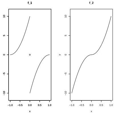
f1(x) = 10(|x| −1)2·sign(x), x∈[−1,1] and, in the second scenario (j=2), the regression function is given by
f2(x) = 10x2·sign(x), x∈[−1,1].
As illustrated in Figure 2, the difference between f1 and f2 is that the parts of the functions on
(−1,0) and (0,1) are interchanged. In both cases, X1, . . . ,Xn are i.i.d. drawn from the uniform
−1.0 −0.5 0.0 0.5 1.0
−10
−5
0
5
10
f_1
x
y
−1.0 −0.5 0.0 0.5 1.0
−10
−5
0
5
10
f_1
x
y
−1.0 −0.5 0.0 0.5 1.0
−10
−5
0
5
10
f_2
x
y
Figure 2: Graph of the regression functions f1(x) =10(|x| −1)2·sign(x)and f2(x) =10x2·sign(x) in model (15)
Classical SVMs, the localized version SVM-KNN, and classical kNN are applied to simulated data sets of size n=200 for both scenarios each with 500 runs. In case of classical SVMs, the Gaussian RBF kernelKγ(x,x′) =exp(−γ(x−x′)2)and theε-insensitive loss forε=0.001 are used. The hyperparameterγis chosen by a five-fold cross validation among
0.001, 0.005, 0.01, 0.05, 0.1, 0.5, 1, 2, 5, 10, 15, 20, 30, 50, 75, 100, 150, 200, 250, 300, 350, 400, 500
and the regularization parameter is equal toλn=a·n−0.45where ais chosen by a five-fold cross
validation among
0.00001, 0.00005, 0.0001, 0.0005, 0.001, 0.005, 0.01, 0.05, 0.1,
The choiceλn=a·n−0.45is motivated by the fact that classical SVMs with theε-insensitive loss are
consistent if limn→∞λn=0 and limn→∞λ2nn=∞; see (Christmann and Steinwart, 2007, Theorem
12). In case of SVM-KNN, the number of nearest neighbors is equal tokn=
b·n0.75where the hyperparameterbis chosen by a five-fold cross validation among
0.15, 0.2 ,0.3 ,0.4 ,0.5 ,0.6 ,0.7 ,0.8 ,0.9 ,1 .
The exponent 0.75 for the definition ofknis in accordance with the settings in Section 3. Choosing
kn =
b·n0.75 would also guarantee universal consistency of classical kNN; see, for example, (Gy¨orfi et al., 2002, Theorem 6.1). For each testing pointξ, the prediction is calculated by a local SVM on theknnearest neighbor. For each local SVM, the polynomial kernelK(x,x′) = (x·x′+1)3
with degree 3 and theε-insensitive loss forε=0.001 are used. In accordance with the settings in Section 3, the regularization parameter is equal toΛn,ξ=Cn,ξmax
0.01k−n0.2, 1
0.01, 0.1, 1, 10, 100, 1000, 10000, 100000 .
Similarly to the case of SVM-KNN, the number of nearest neighbors in the classical kNN method is equal tokn=
c·n0.5where the hyperparametercis chosen by a five-fold cross validation among
0.1, 0.2 ,0.3 ,0.4 ,0.5 ,0.6 ,0.7 ,0.8 ,0.9 ,1 .
The evaluation of the estimates is done on a test data set which consists of 1001 equidistant grid pointsξion[−1,1]. For every runr∈ {1, . . . ,500}, the mean absolute error (MAE) is calculated
MAEj,r(f⋆) = 1
1001 1001
∑
i=1
f⋆(xi)−fj(xi)
for f⋆∈
fSVM
j,r,f
SVM-KNN
j,r ,f
kNN
j,r
where fSVM
j,r denotes the SVM-estimate, fSVM-KNNj,r denotes the SVM-KNN-estimate, and fkNNj,r denotes the
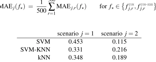
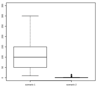
kNN-estimate in ther-th run of scenario j. For every scenario jand every learning algorithm, the values MAEj,r(f⋆),r∈ {1, . . . ,500}, are shown in a boxplot in Figure 3. In addition, Table 1 shows
the average of MAEj,r(f⋆)over the 500 runs:
MAEj(f⋆) =
1 500
500
∑
r=1MAEj,r(f⋆) for f⋆∈
fSVM
j,r,f
SVM-KNN
j,r .
scenario j=1 scenario j=2
SVM 0.453 0.115
SVM-KNN 0.331 0.216
kNN 0.348 0.189
Table 1: The average MAEj of the mean absolute error over the 500 runs for classical SVMs and
SVM-KNN for scenarios j=1 and j=2
It turns out that SVM-KNN is clearly better than classical SVM in scenario 1 while classical SVM is clearly better than KNN in scenario 2. In both examples, the performance of SVM-KNN is similar to that of classical kNN. Function f2in scenario 2 is a smooth function and classical SVMs are typically very successful for learning such smooth functions. Function f1in scenario 1 nearly coincides withf2in scenario 2 in the sense that the parts of the functions on(−1,0)and(0,1)
SVM SVM−KNN kNN
0.0
0.1
0.2
0.3
0.4
0.5
0.6
0.7
Scenario 1
SVM SVM−KNN kNN
0.0
0.1
0.2
0.3
0.4
0.5
0.6
0.7
Scenario 2
Figure 3: Boxplots of the mean absolute errors MAEj,r in the runsr∈ {1, . . . ,500} for classical
SVMs and SVM-KNN for scenarios j=1 and j=2
scenario 1 scenario 2
0
50
100
150
200
250
300
350
Figure 4: Values of the hyperparameterγselected by cross validation for the classical SVM in the 500 runs for each scenario
5. Conclusions
num-−1.0 −0.8 −0.6 −0.4 −0.2 0.0 0 2 4 6 8 10
run r= 1
x
f(x)
−1.0 −0.8 −0.6 −0.4 −0.2 0.0
0 2 4 6 8 10
run r= 1
x
f(x)
−1.0 −0.8 −0.6 −0.4 −0.2 0.0
0 2 4 6 8 10 x f(x)
−1.0 −0.8 −0.6 −0.4 −0.2 0.0
0 2 4 6 8 10
run r= 2
x
f(x)
−1.0 −0.8 −0.6 −0.4 −0.2 0.0
0 2 4 6 8 10
run r= 2
x
f(x)
−1.0 −0.8 −0.6 −0.4 −0.2 0.0
0 2 4 6 8 10 x f(x)
−1.0 −0.8 −0.6 −0.4 −0.2 0.0
0 2 4 6 8 10
run r= 3
x
f(x)
−1.0 −0.8 −0.6 −0.4 −0.2 0.0
0 2 4 6 8 10
run r= 3
x
f(x)
−1.0 −0.8 −0.6 −0.4 −0.2 0.0
0 2 4 6 8 10 x f(x)
−1.0 −0.8 −0.6 −0.4 −0.2 0.0
0 2 4 6 8 10
run r= 4
x
f(x)
−1.0 −0.8 −0.6 −0.4 −0.2 0.0
0 2 4 6 8 10
run r= 4
x
f(x)
−1.0 −0.8 −0.6 −0.4 −0.2 0.0
0 2 4 6 8 10 x f(x)
−1.0 −0.8 −0.6 −0.4 −0.2 0.0
0 2 4 6 8 10
run r= 5
x
f(x)
−1.0 −0.8 −0.6 −0.4 −0.2 0.0
0 2 4 6 8 10
run r= 5
x
f(x)
−1.0 −0.8 −0.6 −0.4 −0.2 0.0
0 2 4 6 8 10 x f(x)
−1.0 −0.8 −0.6 −0.4 −0.2 0.0
0 2 4 6 8 10
run r= 6
x
f(x)
−1.0 −0.8 −0.6 −0.4 −0.2 0.0
0 2 4 6 8 10
run r= 6
x
f(x)
−1.0 −0.8 −0.6 −0.4 −0.2 0.0
0 2 4 6 8 10 x f(x)
−1.0 −0.8 −0.6 −0.4 −0.2 0.0
0 2 4 6 8 10
run r= 7
x
f(x)
−1.0 −0.8 −0.6 −0.4 −0.2 0.0
0 2 4 6 8 10
run r= 7
x
f(x)
−1.0 −0.8 −0.6 −0.4 −0.2 0.0
0 2 4 6 8 10 x f(x)
−1.0 −0.8 −0.6 −0.4 −0.2 0.0
0 2 4 6 8 10
run r= 8
x
f(x)
−1.0 −0.8 −0.6 −0.4 −0.2 0.0
0 2 4 6 8 10
run r= 8
x
f(x)
−1.0 −0.8 −0.6 −0.4 −0.2 0.0
0 2 4 6 8 10 x f(x)
−1.0 −0.8 −0.6 −0.4 −0.2 0.0
0 2 4 6 8 10
run r= 9
x
f(x)
−1.0 −0.8 −0.6 −0.4 −0.2 0.0
0 2 4 6 8 10
run r= 9
x
f(x)
−1.0 −0.8 −0.6 −0.4 −0.2 0.0
0 2 4 6 8 10 x f(x)
Figure 5: Estimates on the interval [−1,0] in the first nine runs in scenario 1: true function f1 (dashed black line), SVM (solid black line), SVM-KNN (solid gray line)
ber of recent articles such localizations of support vector machines have been suggested and their success has empirically been shown in extensive simulation studies and on real data sets but only little has been known on theoretical properties. In this article, it has been shown for a large class of regularized kernel methods (including SVM) that suitably localized versions (called SVM-KNN) are universally consistent.
Instead of localizing support vector machines, it would also be possible in principle to local-ize any other learning algorithm, for example, boosting. If this is done suitably, then localizing a learning algorithm will often lead to an algorithm which is again universally consistent. This article presents one way how this can be done in the special case of regularized kernel methods. However, it is a topic of further research if it is possible to derive a general scheme of localizing learning algo-rithms which, in combination with properties of the learning algorithm, always guarantees universal consistency.
Acknowledgments
Appendix A. Preparations
Let PX denote the distribution of the covariates Xi. For every ζ= (ξ,u)∈
X
×(0,1), there is asmallestrn,ξ∈[0,∞]such thatQ |Xi−ξ| ≤rn,ξ
≥knn and there is ansn,ζ∈[0,∞)such that
Q
|Xi−ξ|<rn,ξ or |Xi−ξ|=rn,ξ,|Ui−u|<sn,ζ
= kn
n .
For everyζ= (ξ,u)∈
X
×(0,1),r∈[0,∞), ands∈[0,∞), define the open ballsBr(ξ) ={x∈X
||x−ξ|<r}andBs(u) ={v∈(0,1)||v−u|<s}, and define the boundary∂Br(ξ) ={x∈
X
||x−ξ|=r}.Define
Bn,ζ =
Brn,ξ(ξ)×(0,1)
∪∂Brn,ξ(ξ)×Bsn,ζ(u)
Roughly spoken, Bn,ζ is a neighborhood around ζ= (ξ,u) with probability kn/nwhich is in line
with our tie-breaking strategy. Then,
PX⊗Unif(0,1) Bn,ζ
= Q Zi∈Bn,ζ
= kn
n
where Unif(0,1)denotes the uniform distribution on(0,1). LetPn,ζbe the conditional distribution of ZigivenZi∈Bn,ζ, that is,
Pn,ζ(B) = Q Zi ∈ B∩Bn,ζ
Q Zi∈Bn,ζ
=
n kn
Q Zi ∈B∩Bn,ζ
∀B∈BX
×(0,1).
Letx7→P(·|x)be any regular version of the factorized conditional distribution ofYigivenXi=x; see,
for example, (Dudley, 2002, § 10.2). Due to independence ofUi, this coincides with the conditional
distribution ofYigivenZi=z(i.e., given(Xi,Ui) = (x,u)) and, accordingly, we writeP(·|z) =P(·|x).
LetQZ,Y denote the joint distribution of(Zi,Yi)and define
Z
:=X
×(0,1). Then, for everyζ∈Z
,n∈N, and every integrableg:
Z
×Y
→R,n kn
Z
Z×YIBn,ζ(z)g(z,y)QZ,Y d(z,y)
=
Z
Z Z
Yg(z,y)P(dy|z)Pn,ζ(dz). (16)
When this does not lead to confusion, the conditional distribution of the pair of random variables
(Zi,Yi)givenZi∈Bn,ζis also denoted byPn,ζ. That is, we will also write
n kn
Z
Z×YIBn,ζ(z)g(z,y)QZ,Y d(z,y)
=
Z
Z×Yg(z,y)Pn,ζ d(z,y)
. (17)
The following lemma is an immediate consequence of the definitions and well known facts about the support of measures, see, for example, Parthasarathy (1967, II. Theorem 2.1). It says that, for almost everyξ∈
X
, the radiirn,ξdecrease to 0.Lemma 2 Define
B0 :=
ξ∈
X
6 ∃r∈(0,∞)such that PX(Br(ξ)) =0 .Then, PX(B0) =1.
Furthermore, for everyξ∈B0,
Similarly to the definition of
I
n,ζandDn,ζ in (4) and (5), we define the modificationsI
⋆n,ζand D⋆n,ζ: For everyn∈N,ζ= (ξ,u)∈
X
×(0,1)andω∈Ω, defineI
n⋆,ζ(ω) :=i∈ {1, . . . ,n}Zi(ω)∈Bn,ζ .
Fix anyn∈N,ζ= (ξ,u)∈
X
×(0,1)andω∈Ωand leti1<i2< . . . <imbe the (ordered) elementsof
I
⋆n,ζ(ω). Then, define
D⋆n,ζ(ω) = Zi1(ω),Yi1(ω)
, . . . , Zim(ω),Yim(ω)
.
That is,
I
n⋆,ζ consists of all those indexes i∈ {1, . . . ,n} andD⋆n,ζ consists of all those data points(Zi,Yi) such that Zi ∈Bn,ζ. This means: while the the sets
I
n,ζ andDn,ζ consist of afixed num-ber of nearest neighbors, the setsI
⋆n,ζ andD⋆n,ζ consist of all those neighbors which lie in afixed neighborhood.
As the probability that Zi ∈Bn,ζ is kn/n, we expect that, for large n, the index sets
I
n,ζ andI
⋆n,ζ and the vectors of data pointsDn,ζ andD⋆n,ζ are similar. However, working with
I
n⋆,ζ is more comfortable because, whether i∈I
n⋆,ζ, only depends on Zi but, whether i∈I
n,ζ, depends on allZ1, . . . ,Zn.
If a real-valued function f is clipped at M, then the clipped version is denoted by af, that is, a
f(x) =f(x)if−M≤f(x)≤M, andaf(x) =−Mif f(x)<−M, andaf(x) =MifM<f(x). Note that,
for every f1,f2 :
X
→Randξ∈X
, it follows thata
f1(ξ)−af2(ξ)≤
f1(ξ)−f2(ξ)
. Furthermore,
sinceKis bounded, every f∈Hfulfills|f(ξ)| ≤ kKk∞·kfkH; see (Steinwart and Christmann, 2008,
Lemma 4.23). In combination with (12), this implies that, for everyξ∈
X
and for every f1,f2∈H,
Z
L y,af1(ξ)
P(dy|ξ)−
Z
L y,af2(ξ)
P(dy|ξ)
≤ |L|M,1·kKk∞·kf1−f2kH. (18)
DefinekL(·,0)k∞=supy∈[−M,M] L(y,0)
. Then, for every probability measureP0,
R
P0(0) =Z
L(y,0)P0 d(x,y)
≤ kL(·,0)k∞
(13)
< ∞. (19)
The following lemma is one of the main tools; it is an application of Hoeffding’s inequality and will be used several times forV =HandV =R.
Lemma 3 Let V be a separable Hilbert space and, for every n∈N, let Ψn:
Z
×Y
→V be a Borel-measurable function such that for every bounded subset B⊂Z
,sup
n∈N sup
z∈B,y∈Y
Ψn(z,y)
H < ∞.
Then, for everyζ∈
X
,λ−32
n
n kn
1 n
n
∑
i=1Ψn(Zi,Yi)IBn,ζ(Zi)−
Z
Ψn(z,y)IBn,ζ(z)QZ,Y d(z,y)
!
−−−→n
→∞ 0
Note that the integral in Lemma 3 is an integral over a Hilbert-space-valued function and, accord-ingly, is a Bochner integral; see, for example, (Denkowski et al., 2003, § 3.10) for such integrals. Proof The proof is done by an application of Hoeffding’s inequality for functions with values in a separable Hilbert space. According to Lemma 2, there is ann0∈Nsuch thatBn
0,ζis bounded and Bn,ζ⊂Bn0,ζfor everyn≥n0. Hence, there is a constantb∈(0,∞)such that, for everyn≥n0,
sup
(z,y)∈Z×Y
Ψn(z,y)IB
n,ζ(z)
V ≤b.
For everyn≥n0andτ∈(0,∞), define an,τ :=2b·
√
τn−1+√n−1+τn−1
and
An,τ=
(
1 n
n
∑
i=1Ψn(Zi,Yi)IBn,ζ(Zi)−
Z
ΨnIBn,ζdQZ,Y
V
<an,τ
)
.
Then, by Hoeffding’s inequality for separable Hilbert spaces (e.g., Steinwart and Christmann, 2008, Corollary 6.15),
Q An,τ
≥ 1−e−τ ∀n≥n0, ∀τ∈(0,∞). (20)
Defineτn:=λ
3 2
nknn−
1
2 andεn:=λ− 3 2
n nk−n1an,τn for everyn≥n0. Then, for everyω∈An,τ,
λ−32
n
n kn
1 n
n
∑
i=1Ψn(Zi(ω),Yi(ω))IBn,ζ(Zi(ω))−
Z
ΨnIBn,ζdQZ,Y
V
< εn.
According to (9),
εn=
n·an,τn
λ32
nkn
= 2bn
λ32
nkn
s
λ32
nkn √
nn+
r
1 n+
λ32
nkn √
nn
!
=2b·
s √
n
λ32
nkn
+
√
n
λ32
nkn
+√1
n
!
−−−→n
→∞ 0.
Hence, for everyε>0, there is annε∈Nsuch thatε>εnfor everyn≥nεand, therefore,
Q λ−32
n
n kn
1 n
n
∑
i=1Ψn(Zi,Yi)IBn,ζ(Zi)−
Z
ΨnIBn,ζdQZ,Y
V
>ε
!
≤Q∁An,τ
n
(20)
≤ e−τn.
The last expression converges to 0 because limn→∞τn=∞due to (9),
Appendix B. Measurability
Lemma 4
(a) The following maps are measurable with respect to the product-σ-algebraBp⊗B(0,1)⊗
A
and the respective Borel-σ-Algebra:
(i) Rp×(0,1)×Ω → R(p+1)kn, (ξ,u,ω) = (ζ,ω) 7→ Dn,ζ(ω)
(ii) Rp×(0,1)×Ω → R, (ξ,u,ω) = (ζ,ω) 7→ Rn,ζ(ω) := maxi∈I
n,ζ
Xi(ω)−ξ .
(iii) Rp×(0,1)×Ω → R, (ξ,u,ω) = (ζ,ω) 7→ Λ˜n,ζ(ω).
(b) Let Λ:Rp×(0,1)×Ω→ (0,∞) be measurable with respect to Bp⊗B(0,1)⊗
A
and the Borel-σ-Algebra. Then,Rp×(0,1)×Ω → R, (ξ,u,ω) = (ζ,ω) 7→ fD
n,ζ(ω),Λ(ζ,ω)(ξ)
is measurable with respect toBp⊗B(0,1)⊗
A
andB.(c) For everyζ= (ξ,u)∈Rp×(0,1)and everyΛ:Ω→(0,∞)measurable with respect to
A
and the Borel-σ-Algebra, the mapΩ → R, ω 7→ fD⋆
n,ζ(ω),Λ(ω)(ξ)
is measurable with respect to
A
andB.Proof For everyζ= (ξ,u)∈Rp×(0,1)andω∈Ω, define
I
n,ζ(ω)as in Section 2. Let Indndenote
the set of all subsets of{1, . . . ,n}withknelements. First, it is shown that
˜
τn:Ω×Rp×(0,1) → Indn, (ω,ξ,u) 7→
I
n,(ξ,u)(ω)is measurable with respect to
A
⊗Bp⊗B(0,1)and 2Indn: Take any
I
∈Indnsuch thatI
6={1, . . . ,kn}and, for every
J
⊂ {1, . . . ,n}, defineB(J1) := n(ω,ξ,u)∈Ω×Rp×(0,1) maxi
∈I |Xi(ω)−ξ| ≤minℓ6∈I |Xℓ(ω)−ξ|
o
B(J2) := n(ω,ξ,u)∈Ω×Rp×(0,1)
|Xj(ω)−ξ|=maxi
∈I |Xi(ω)−ξ| ∀j∈
J
o
B(J3) := n(ω,ξ,u)∈Ω×Rp×(0,1)
|Xℓ(ω)−ξ| 6=max
i∈I |Xi(ω)−ξ| ∀ℓ6∈
J
o
B(J4) := n(ω,ξ,u)∈Ω×Rp×(0,1)
max
i∈J∩I|Ui(ω)−u|<jmin∈J\I|Uj(ω)−u|
o .
The setB(J1)says that noXℓis closer toξthan theknnearest neighbors. The setsB(J2)andB
(3)
J states
that
J
specifies all thoseXjwhich lie at the border of the neighborhood given by the nearestneigh-bors. The setB(J4)is concerned with all data points which lie at the border: the nearest neighbors among them have strictly smaller|Ui−u|than those which do not belong to the nearest neighbors.
Accordingly, the inverse image ˜τ−1
n ({
I
})equals˜ τ−1
n ({
I
}) =[
J⊂{1,...,n}
Since B(Jt) is measurable for everyt∈ {1,2,3,4} and
J
⊂ {1, . . . ,n}, this shows that ˜τ−1n ({
I
}) ismeasurable for every
I
6={1, . . . ,kn}. Hence, ˜τnis measurable. For everyI
={i1, . . . ,ikn}such thati1<i2<···<ikn and everyDn= (z1,y1), . . . ,(zn,yn)
∈((Rp×(0,1))×R)ndefine
ϕn(
I
,Dn) = (zi1,yi1), . . . ,(zikn,yikn).
The map ϕn : Indn×((Rp×(0,1))×R)n→((Rp×(0,1))×R)kn is continuous (where Indn is
endowed with the discrete topology). Since
Dn,ζ(ω) = ϕn
˜
τn(ω,ξ,u),Dn(ω)
forζ= (ξ,u),
statement (i) follows from measurability of ˜τn and ϕn. Next, (ii) follows from measurability of
(xi1, . . . ,xikn,ξ)7→maxj∈{1,...,kn}|xij−ξ|and (iii) follows from
˜
Λn,ζ = 1
kn n
∑
i=1|Xi−ξ|
3 2I
[0,∞)(Rn,ζ−Xi).
Now, we can prove part (b) and (c): For every
I
⊂ {1,2, . . . ,n}and everyD= (x1,y1), . . . ,(xn,yn)
∈
((Rp×(0,1))×R)n, denoteDI = (xi,yi)
i∈I. Then, it follows from Lemma 9 (a) and (Steinwart
and Christmann, 2008, Lemma 4.23) that the map
2{1,2,...,n}×((Rp×(0,1))×R)n×
X
→ H, (I
,D,ξ) 7→ fDI,λ(ξ)is continuous for every λ>0 (where 2{1,2,...,n} is endowed with the discrete topology). Since λ7→ fDI,λ(ξ)is continuous for every fixed(
I
,D,ξ)according to (Steinwart and Christmann, 2008,Corollary 5.19 and Lemma 4.23), the map (
I
,D,ξ),λ7→ fDI,λ(ξ) is a Caratheodory function
and, therefore, measurable; see, for example, Denkowski et al. (2003, Definition 2.5.18 and Theo-rem 2.5.22). Then, (b) follows from (a), and (c) follows from measurability of ˜τ∗n,ζ:ω7→
I
n∗,ζ(ω)for every fixedζ= (ξ,u). Measurability of ˜τ∗
n,ζfollows from
˜
τ∗n,ζ−1(
I
) = \i∈I
Zi−1(Bn,ζ)∩
\
i6∈I
Z−i 1(∁Bn,ζ) ∀
I
∈2{1,2,...,n}.Appendix C. Proof of Theorem 1
In the main part of the proof, it is shown that forPX⊗Unif(0,1)- almost everyζ= (ξ,u)∈
X
×(0,1),0≤ Z
L y,afDn,ζ,Λn,ζ(ξ)
P(dy|ζ)−inf
t∈R Z
L(y,t)P(dy|ζ) −−−→
n→∞ 0 (21)
in probability. Then, statement (21) implies Theorem 1 as follows: Since, for every fixedζ= (ξ,u), the maps
ω 7→
Z
L y,afDn,ζ(ω),Λn,ζ(ω)(ξ)
P(dy|ζ)−inf
t∈R Z
are uniformly bounded, convergence in probability for PX⊗Unif(0,1)- almost every ζ= (ξ,u)∈
X
×(0,1)impliesEQ
Z
L y,afDn,ζ,Λn,ζ(ξ)
P(dy|ζ)− inf
t∈R Z
L(y,t)P(dy|ζ)
−−−→n
→∞ 0
forPX⊗Unif(0,1)- almost everyζ= (ξ,u)∈
X
×(0,1). Since the mapsζ= (ξ,u) 7→ EQ
Z
L y,afDn,ζ,Λn,ζ(ξ)
P(dy|ζ)− inf
t∈R Z
L(y,t)P(dy|ζ)
, n∈N,
are uniformly bounded again,PX⊗Unif(0,1)- almost sure convergence implies
ZZ
EQ
Z
L y,afDn,ζ,Λn,ζ(ξ)
P(dy|ζ)−inf
t∈R Z
L(y,t)P(dy|ζ)
PX(dξ)Unif(0,1)(du)−→ 0 (22)
forn→∞. Note thatζ7→inft∈R R
L(y,t)P(dy|ζ)is measurable, because the assumptions onLimply continuity oft7→RL(y,t)P(dy|ζ), hence, inft∈RRL(y,t)P(dy|ζ) =inft∈QRL(y,t)P(dy|ζ)for every
ζ∈
X
×(0,1). Next, recall that fDn(ζ) =a
fDn,ζ,Λn,ζ(ξ)andP(·|ξ) =P(·|ζ)for everyζ= (ξ,u). By a slight abuse of notation, we write
R
P(fDn) =R
P⊗Unif(0,1)(fDn) = ZZL y,fDn(ξ,u)
P d(ξ,y)
Unif(0,1)(du).
Then, applying Fubini’s Theorem in (22) yields
0 ≤ EQ
R
P fDn
− Z
inf
t∈R Z
L(y,t)P(dy|ξ)PX(dξ)
−−−→n
→∞ 0. (23)
For every measurable f :
X
→R,Z
L y,f(ξ)
P(dy|ξ) ≥ inf
t∈R Z
L(y,t)P(dy|ξ) ∀ξ∈
X
.Hence,
R
P∗ ≥ Zinf
t∈R Z
L(y,t)P(dy|ξ)PX(dξ)
and, therefore, (23) implies
EQ
R
P fDn
−
R
P∗−−−→n
→∞ 0
and, as
R
P fDn
≥
R
P∗,EQ
R
P fDn−
R
P∗−−−→
n→∞ 0.
In particular, this also implies
R
P fDn
−−−→n
→∞
R
∗That is, it only remains to prove (21). To this end, note that, for everyζ= (ξ,u)∈
X
×(0,1), we haveP(·|ζ) =P(·|ξ)and0 ≤ Z
L y,afDn,ζ,Λn,ζ(ξ)
P(dy|ζ)− inf
t∈R Z
L(y,t)P(dy|ζ) ≤
≤ Z
L y,afDn,ζ,Λn,ζ(ξ)
P(dy|ξ)−
Z
L y,afD⋆
n,ζ,Λn,ζ(ξ)
P(dy|ξ) (24) + Z
L y,afD⋆
n,ζ,Λn,ζ(ξ)
P(dy|ξ)−
Z
L y,afPn,ζ,Λn,ζ(ξ)
P(dy|ξ) (25) + Z
L y,afPn,ζ,Λn,ζ(ξ)
P(dy|ξ)−
ZZ
L y,afPn,ζ,Λn,ζ(x)
P(dy|x)Pn,ζ(d(x,v))
(26) + ZZ
L y,afPn,ζ,Λn,ζ(x)
P(dy|x)Pn,ζ(d(x,v))−inf
t∈R Z
L(y,t)P(dy|ξ)
∨0 (27)
where a∨0=max{a,0}. Therefore, it suffices to prove convergence in probability of each of these four summands. This is done in the following four subsections but, first, we need some more preparations:
Lemma 5 Fix anyζ= (ξ,u)∈B0×(0,1)where B0 is defined as in Lemma 2. LetPD
n,ζ andPD⋆n,ζ denote the empirical measure corresponding toDn,ζandD⋆n,ζrespectively. It follows that
λ−32
n
♯(
I
⋆n,ζ)−kn
kn −−−→n→∞
0 in probability, (28)
λ−32
n
♯(
I
n⋆,ζ)−kn♯(
I
⋆n,ζ)
−−−→n
→∞ 0 in probability, (29)
λ−32
n
PDn,ζ−PD⋆n,ζ
TV −−−→n→∞ 0 in probability, (30)
Rn,ζ := max
i∈In,ζ|
Xi−ξ| −−−→
n→∞ 0 in probability, (31)
and, for everyβ∈(0,∞),
λ−32
n 1 kni∈
∑
In,ζ|Xi−ξ|β− Z
|x−ξ|βPn,ζ(d(x,v))
−−−→n→∞
0 in probability. (32)
Proof Statement (28) follows from Lemma 3 because the definitions imply
λ− 3 2
n
♯(
I
⋆n,ζ)−kn
kn
= λ−
3 2 n n kn 1 n n
∑
i=1IBn,ζ(Zi)−
Z
IBn,ζ(z)QZ,Y d(z,y)

![Figure 5: Estimates on the interval [−1,0] in the first nine runs in scenario 1: true function f1(dashed black line), SVM (solid black line), SVM-KNN (solid gray line)](https://thumb-us.123doks.com/thumbv2/123dok_us/9811900.1967055/13.612.102.505.94.371/figure-estimates-interval-rst-scenario-function-dashed-solid.webp)
