Semi-Supervised Learning Using Greedy Max-Cut

Semi-Supervised Learning Using Greedy Max-Cut

Jun Wang [email protected]

IBM T.J. Watson Research Center 1101 Kitchawan Road

Yorktown Heights, NY 10598, USA

Tony Jebara [email protected]

Department of Computer Science Columbia University

New York, NY 10027, USA

Shih-Fu Chang [email protected]

Department of Electrical Engineering Columbia University

New York, NY 10027, USA

Editor:Mikhail Belkin

Abstract

Graph-based semi-supervised learning (SSL) methods play an increasingly important role in prac-tical machine learning systems, particularly in agnostic settings when no parametric information or other prior knowledge is available about the data distribution. Given the constructed graph rep-resented by a weight matrix, transductive inference is used to propagate known labels to predict the values of all unlabeled vertices. Designing a robust label diffusion algorithm for such graphs is a widely studied problem and various methods have recently been suggested. Many of these can be formalized as regularized function estimation through the minimization of a quadratic cost. However, most existing label diffusion methods minimize a univariate cost with the classification function as the only variable of interest. Since the observed labels seed the diffusion process, such univariate frameworks are extremely sensitive to the initial label choice and any label noise. To alleviate the dependency on the initial observed labels, this article proposes a bivariate formulation for graph-basedSSL, where both the binary label information and a continuous classification func-tion are arguments of the optimizafunc-tion. This bivariate formulafunc-tion is shown to be equivalent to a linearly constrained Max-Cut problem. Finally an efficient solution via greedy gradient Max-Cut (GGMC) is derived which gradually assigns unlabeled vertices to each class with minimum con-nectivity. Once convergence guarantees are established, this greedy Max-Cut basedSSLis applied on both artificial and standard benchmark data sets where it obtains superior classification accu-racy compared to existing state-of-the-artSSLmethods. Moreover,GGMCshows robustness with respect to the graph construction method and maintains high accuracy over extensive experiments with various edge linking and weighting schemes.

Keywords: graph transduction, semi-supervised learning, bivariate formulation, mixed integer

programming, greedy Max-Cut

1. Introduction

In many real applications, labeled samples are scarce but unlabeled samples are abundant. Paradigms

been increasingly explored in practical machine learning systems. While many semi-supervised learning approaches estimate a smooth function over labeled and unlabeled examples, this article

presents a novel approach which emphasizes abivariateoptimization problem over the

classifica-tion funcclassifica-tionandthe labels. Prior to describing the method in detail, we briefly mention otherSSL

methods and previous work to motivate this article’s contributions.

One of the earliest examples of the empirical advantages ofSSLwas co-training, a method first

developed for text mining problems (Blum and Mitchell, 1998) and later extended in various forms to other applications (Chawla and Karakoulas, 2005; Goldman and Zhou, 2000). Therein, multi-ple classifiers are first estimated using conditionally independent feature sets of training data. The performance advantages of this method rely heavily on the existence of independent and comple-mentary classifiers. Theoretical results show that some mild assumptions on the underlying data distribution are sufficient for co-training to work (Balcan et al., 2005; Wang and Zhou, 2010). How-ever, performance can dramatically degrade if the classifiers do not complement each other or the independence assumption does not hold (Krogel and Scheffer, 2004). Though co-training is concep-tually similar to semi-supervised learning due to the way it incorporates unlabeled data, the classifier training procedure itself is often supervised.

The extension of traditional supervised support vector machines (SVMs) to the semi-supervised

scenario is another widely usedSSLalgorithm. Instead of maximizing separation (via a

maximum-margin hyperplane) over training data as in standard SVMs, semi-supervised SVMs (S3VMs)

es-timate a hyperplane to balance maximum-margin partitioning of labeled data while encouraging a separation through low-density regions of the data (Vapnik, 1998). For example, transductive support vector machines (TSVMs) were developed as one of the earliest incarnations of

semi-supervisedSVMs (Joachims, 1999).1 Various optimization techniques have been applied to solve

S3VMs(Chapelle et al., 2008), resulting in a wide range of methods, such as low density separation (Chapelle and Zien, 2005), semi-definite programming based methods (Bie and Cristianini, 2004; Xu et al., 2008), and a branch-and-bound based approach (Chapelle et al., 2007).

Another family ofSSLmethods known as graph-based approaches have recently become

popu-lar due to their high accuracy and computational efficiency. Graph-based semi-supervised learning

(GSSL) treats both labeled and unlabeled samples from a data set as vertices in a graph and builds

pairwise edges between these vertices which are weighted by the affinity between the corresponding

samples. The small portion of vertices with labels are then used bySSLmethods to perform graph

partition or information propagation to predict labels for unlabeled vertices. For instance, the graph mincuts approach formulates the label prediction as a graph cut problem (Blum and Chawla, 2001;

Blum et al., 2004). OtherGSSLmethods, like graph transductive learning, formulate the problem

as regularized function estimation over an undirected weighted graph. These methods optimize a trade-off between the accuracy of the classification function on labeled samples and a regulariza-tion term that favors a smooth funcregulariza-tion. The weighted graph and the optimal funcregulariza-tion ultimately propagate label information from labeled data to unlabeled data to produce transductive

predic-tions. Popular algorithms forGSSLinclude graph cuts (Blum and Chawla, 2001; Blum et al., 2004;

Joachims, 2003; Kveton et al., 2010), graph random walks (Azran, 2007; Szummer and Jaakkola, 2002), manifold regularization (Belkin et al., 2005, 2006; Sindhwani et al., 2008, 2005), and graph regularization (Zhou et al., 2004; Zhu et al., 2003). Comprehensive survey articles have also been disseminated (Zhu, 2005).

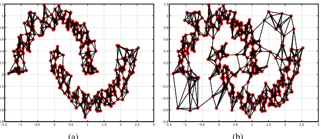
For some synthetic and real data problems, GSSL approaches do achieve promising perfor-mance. However, previous research has identified several realistic settings and labeling situations where this performance can be compromised (Wang et al., 2008b). In particular, both the graph construction methodology and the label initialization conditions can significantly impact prediction accuracy (Jebara et al., 2009). For a well-constructed graph such as the one shown in Figure 1(a),

manyGSSLmethods produce satisfactory predictions. However, for graphs involving non-separable

manifold structure as shown in Figure 1(b), prediction accuracy may deteriorate. Even if one as-sumes that the graph structures used in the above methods faithfully describe the data manifold,

GSSLalgorithms may still be misled by problems in the label information. Figure 3 depicts several

cases where the label information leads to invalid graph transduction solutions for all the aforemen-tioned algorithms.

In order to handle such challenging labeling conditions, we first extend the existingGSSL

for-mulation by casting it as abivariateoptimization problem over the classification functionandthe

labels. Then we demonstrate that minimizing the mixed bivariate cost function can be reduced to a pure integer programming problem that is equivalent to a constrained Max-Cut problem. Though semi-definite programming can be used to obtain approximate solutions, these are impractical due

to scalability issues. Instead, an efficient greedy gradient Max-Cut (GGMC) solution is developed

which remedies the instability previous methods seem to have vis-a-vis the initial labeling condi-tions on the graph. In the proposed greedy solution, initial labels simply act as initial values of the graph cut which is incrementally refined until convergence. During each iteration of the greedy search, the optimal unlabeled vertex is assigned to the labeled subset with minimum connectivity to maximally preserve cross-subset edge weight. Finally, an overall cut is produced after placing the unlabeled vertices into one of the label sets. It is then straightforward to obtain the final label prediction from the graph cut result. Note that this greedy gradient Max-Cut solution is equivalent to alternating between minimization of the cost over the label matrix and minimization of the cost over the prediction function. Moreover, to alleviate dependencies on the initialization of the cut (the given labels), a re-weighting of the connectivity between unlabeled vertices and labeled subsets is proposed. This re-weighting performs a within-class normalization using vertex degree as well as a between-class normalization using class prior information. We demonstrate that the greedy gradient Max-Cut based graph transduction produces significantly better performance on both artificial and real data sets.

The remainder of this paper is organized as the follows. Section 2 provides a brief background

of graph-basedSSLand discusses some open issues. In Section 3, we present our bivariate graph

transduction framework, followed by the theoretical proof of its equivalence with the constrained Max-Cut problem in Section 4. In addition, a greedy gradient Max-Cut algorithm is proposed. Section 5 provides experimental validation for the algorithm on both toy and real classification data sets. Comparisons with leading semi-supervised methods are made. Concluding remarks and discussions are then provided in Section 6.

2. Background and Open Issues

In this section, we introduce some notation and then revisit two critical components of graph-based

SSL: graph construction and label propagation. Subsequently, we discuss some challenging issues

−1.5 −1 −0.5 0 0.5 1 1.5 2 2.5 3 −0.8

−0.6 −0.4 −0.2 0 0.2 0.4 0.6 0.8 1 1.2

(a)

−1.5 −1 −0.5 0 0.5 1 1.5 2 2.5 3

−0.8 −0.6 −0.4 −0.2 0 0.2 0.4 0.6 0.8 1 1.2

(b)

Figure 1: Examples of constructed k-nearest-neighbors (kNN) graphs with k=5 on the artificial

two moon data set for a) the completely separable case; and b) the non-separable case with noisy samples.

2.1 Notations

We first summarize the notation used in this article. Assume we are giveniid(independent and

iden-tically distributed) labeled samples _{(x1,z1), . . . ,(xl,zl)} as well as unlabeled samples

{xl+1, . . . ,xl+u}drawn from a distributionp(x,z). Define the set of labeled inputs asXl={x1, . . . ,xl}

with cardinality_|Xl|=land the set of unlabeled inputsXu={xl+1, . . . ,xl+u}with cardinality|Xu|=

u. The labeled setXlis associated with labels

Z

l={z1,···,zl}, wherezi∈ {1,···,c},i=1,2,···,l.

The goal of semi-supervised learning is to infer the missing labels_{zl+1,···,zn}corresponding to

the unlabeled data _{xl+1,···,xn}, where typically l<<n (l+u=n). A crucial component of

GSSL is the estimation of a weighted sparse graph

G

from the input data X=Xl∪Xu.

Subse-quently, a labeling algorithm uses

G

and the known labels

Z

l ={z1, . . . ,zl} to provide estimates

ˆ

Z

u={zˆl+1, . . . ,zˆl+u}which try to approximate the true labels

Z

u={zl+1, . . . ,zl+u}as measured by

an appropriately chosen loss function.

In this article, assume the undirected graph converted from the data X is represented by

G

= _{X,E_}, where the set of vertices isX=_{xi}and the set of edges isE={ei j}. Each samplexi

is treated as a vertex and the weight of edgeei jiswi j. Typically, one uses a kernel functionk(·)over

pairs of points to compute weights. The weights for edges are used to build a weight matrix which

is denoted byW=_{wi j}. Similarly, the vertex degree matrixD=diag([d1,···,dn])is defined as

di= n

∑

j=1

wi j. The graph Laplacian is defined as∆∆∆=D−Wand the normalized graph Laplacian is

L=D−1/2∆∆∆D−1/2=I₋D−1/2WD−1/2.

The graph Laplacian and its normalized version can be viewed as operators on the space of functions

f which can be used to define a regularization measure of smoothness over strongly-connected

regions in a graph (Chung and Biggs, 1997). For example, the smoothness measurement of functions

f usingLover a graph is defined as

hf,Lf_i=

_∑

i

∑

j

wi j

f(xi) √

di −

f(xj) √

dj

Finally, the label information is formulated as a label matrixY=_{yi j} ∈Bn×c, whereyi j =1

if samplexi is associated with label jfor j∈ {1,2,···,c}, that is,zi= j, andyi j =0 otherwise.

For single label problems (as opposed to multi-label problems), the constraints ∑c

j=1

yi j =1 are also

imposed. Moreover, we will often refer to row and column vectors of such matrices, for instance,

thei’th row and j’th column vectors ofYare denoted as Yi· andY·j, respectively. LetF= f(X)

be the values of classification function over the data set X. Most of the GSSL methods then use

the graph quantityW as well as the known labels to recover a continuous classification function

F_∈Rn×cby minimizing a predefined cost on the graph.

2.2 Graph Construction for Semi-Supervised Learning

To estimate ˆ

Z

u={zˆl+1, . . . ,zˆl+u}using

G

and the known labels

Z

l={z1, . . . ,zl}, we first convert the

data pointsX=Xl∪Xuinto a graph

G

={X,E,W}. This section discusses the graph construction

method, X_→

G

, in detail. Given input data X with cardinality _|X_|=l+u, graph construction

produces a graph

G

consisting ofn=l+uvertices where each vertex is associated with the sample

xi. The estimation of

G

fromXusually proceeds in two steps.

The first step is to compute a score between all pairs of vertices using a similarity function. This

creates a full adjacency matrixK_∈Rn×n, whereKi j =k(xi,xj)is computed using kernel function

k(_·)to measure sample similarity. Subsequently, in the second step of graph construction, the matrix

Kis sparsified and reweighted to produce the final matrixW. Sparsification is important since it

leads to improved efficiency, better accuracy, and robustness to noise in the label inference stage.

Furthermore, the kernel functionk(_·)is often only locally useful as a similarity and does not recover

reliable weights between pairs of samples that are relatively far apart.

2.2.1 GRAPHSPARSIFICATION

Starting with the fully connected matrix K, sparsification removes edges by recovering a binary

matrixB_∈Bn×n whereBi j =1 indicates that an edge is present between samplexi andxj, and

Bi j=0 indicates the edge is absent (assumeBii=0 unless otherwise noted). Here we will primarily

investigate two graph sparsification algorithms: neighborhood approaches including the k-nearest

and ε neighbors algorithms, and matching approaches such as b-matching (BM) (Edmonds and

Johnson, 2003). All such methods operate on the matrixK or, equivalently, the distance matrix

H_∈Rn×nobtained fromKelement-wise asHi j=pKii+Kj j−2Ki j.

Sparsification via Neighborhood Methods:There are two typical ways to build a neighborhood

graph: theε-neighborhood graph connecting samples within a distance ofε, and thekNN (k

-nearest-neighbors) graph connectingk closest samples. Recent studies show the dramatic influences that

different neighborhood methods have on clustering techniques (Carreira-Perpin´an and Zemel, 2005;

Maier et al., 2009). In practice, thekNN graph remains a more common approach since it is more

adaptive to scale variation and data density anomalies while an improper threshold value in the

ε-neighborhood graph may result in disconnected components or subgraphs in the data set or even

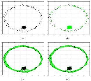
isolated singleton vertices, as shown in Figure 2(b). In this article, we often usekNN neighborhood

graphs since theε-neighborhood graphs provide consistently weaker performance. In the remainder

of this article, we will use neighborhood and kNN neighborhood graph interchangeably without

0.1 0.2 0.3 0.4 0.5 0.6 0.7 0.8 0.1

0.2 0.3 0.4 0.5 0.6 0.7 0.8 0.9

(a)

0.1 0.2 0.3 0.4 0.5 0.6 0.7 0.8

0.1 0.2 0.3 0.4 0.5 0.6 0.7 0.8 0.9

(b)

0.1 0.2 0.3 0.4 0.5 0.6 0.7 0.8

0.1 0.2 0.3 0.4 0.5 0.6 0.7 0.8 0.9

(c)

0.1 0.2 0.3 0.4 0.5 0.6 0.7 0.8

0.1 0.2 0.3 0.4 0.5 0.6 0.7 0.8 0.9

(d)

Figure 2: The synthetic data set used for demonstrating different graph construction approaches. a)

The synthetic data; b) Theε-nearest neighbor graph; c) Thek-nearest neighbor graph; d)

Theb-matched graph.

More specifically, the k-nearest neighbor graph is a graph in which two vertices xi andxj are

connected by an edge if the distanceHi j betweenxi andxj is within or equalk-th smallest among

the distances fromxi to other samples inX. Roughly speaking, thek-nearest neighbors algorithm

starts with a matrix ˆBof all zeros and for each point, searches for thekclosest points to it (without

considering itself). If a point jis one of the k closest neighbors to i, then we set ˆBi j =1. It is

straightforward to show thatk-nearest neighbors search solves the following optimization problem:

min

ˆ

B∈B

∑

i j

ˆ

Bi jHi j (1)

s.t.

_∑

_jBˆi j=k,Bˆii=0,∀i,j∈1, . . . ,n.

The final solution of Equation (1) is produced by symmetrizing ˆBas followsBi j =max(Bˆi j,Bˆji).2

This greedy algorithm is in fact not solving a well defined optimization problem over symmetric

binary matrices. In addition, since it produces a symmetric matrix only via thead hocmaximization

over ˆBand its transpose, the solution Bit produces does not satisfy the equality∑kBi j =k, but,

rather, only satisfies the inequality ∑jBi j ≥k. Ironically, despite conventional wisdom and the

nomenclature, the k-nearest neighbors algorithm is producing an undirected subgraph with more

2. It is possible to replace the maximization operator with minimization to produce a symmetric matrix, yet in the setting

thankneighbors for each vertex. This motivates researchers to investigate theb-matching algorithm which actually achieves the desired output.

Sparsification via b-Matching: The b-matching problem generalizes maximum weight match-ing, that is, the linear assignment problem, where the objective is to find the binary matrix to mini-mize the optimization problem

min

B∈B

∑

i jBi jHi j (2)

s.t.

_∑

_jBi j=b,Bii=0,Bi j=Bji,∀i,j∈1, . . . ,n.

achieving symmetry directly without post-processing. Here, the symmetric solution is recovered

up-front by enforcing the additional constraints Bi j =Bji. The matrix then satisfies the equality

∑jBi j=∑iBi j=bstrictly. The solution to Equation (2) is not quite as straightforward or efficient

as the greedyk-nearest neighbors algorithm. A polynomial time

O

(bn3)solution has been known,

yet recent advances show that much faster alternatives are possible via (guaranteed) loopy belief propagation (Huang and Jebara, 2007).

Compared with the neighborhood graphs, the b-matching graph is balanced or b-regular. In

other words, each vertex in theb-matched graph has exactlybedges connecting it to other vertices.

This advantage plays a key role when conducting label propagation on typical samplesXwhich are

unevenly and non-uniformly distributed. Our previous work appliedb-matching to construct graphs

for semi-supervised learning tasks and demonstrated the superior performance over some unevenly sampled data (Jebara et al., 2009). For example, in Figure 2, this data set clearly contains two clusters of points, a dense Gaussian cluster surrounded by a ring cluster. Furthermore, the cluster

data is unevenly sampled; one cluster is dense and the other is fairly sparse. In this example, thek

-nearest neighbor graph constantly generates many cross-cluster edges whileb-matching efficiently

alleviates this problem by removing most of the improper edges. The example clearly shows that

theb-matching technique produces regular graphs which could overcome the drawback of

cross-structure linkages often generated by nearest neighbor methods. This intuitive study confirms the

importance of graph construction methods and advocatesb-matching as a valuable alternative to

k-nearest neighbors, a method that many practitioners expect to produce regular undirected graphs,

though in practice often generates irregular graphs.

2.2.2 GRAPHEDGERE-WEIGHTING

Once a graph has been sparsified and a binary matrixBis computed and used to delete unwanted

edges, several procedures can then be used to update the weights in the matrixKto produce a final

set of edge weightsW. Specifically, wheneverBi j =0, the edge weight is alsowi j=0; however,

Bi j=1 implies thatwi j ≥0. Two popular approaches are considered here for estimating the

non-zero components ofW.

Binary Weighting:The simplest approach for building the weighted graph is thebinary weight-ing approach, where all the linked edges in the graph are given the weight 1 and the edge weights

of disconnected vertices are given the weight 0. In other words, this setting simply usesW=B.

However, this uniform weight on graph edges can be sensitive, particularly if some of the graph vertices were improperly connected by the sparsification procedure (either the neighborhood based

procedures or theb-matching procedure).

samplesxiandxjis computed as:

wi j=Bi jexp

−d 2_(x

i,xj)

2σ2

,

where the function d(xi,xj) evaluates the dissimilarity of samplesxi and xj, andσ is the kernel

bandwidth parameter. There are many choices for the distance functiond(_·)including anyℓp

dis-tance,χ2_{distance, and cosine distance (Zhu, 2005; Belkin et al., 2005; Jebara et al., 2009).}

This final step in the graph construction procedure ensures that the unlabeled dataXhas now

been converted into a graph

G

with a weighted sparse undirected adjacency matrixW. Given this

graph and some initial label informationYl, any of the current popular algorithms for graph based

SSL can be used to solve the labeling problem.

2.3 Univariate Graph Regularization Framework

Given the constructed graph

G

=_{X,E_}, whose geometric structure is represented by the weight

matrixW, the label inference task is to diffuse the known labels

Z

l to all the unlabeled vertices

Xuin the graph and estimate ˆ

Z

u. Designing a robust label diffusion algorithm for such graphs is a

widely studied problem (Chapelle et al., 2006; Zhu, 2005; Zhu and Goldberg, 2009).

Here we are particularly interested in a category of approaches, which estimate the prediction

functionF_∈Rn×c_{by minimizing a quadratic cost defined over the graph. The cost function typically}

involves a trade-off between the smoothness of the function over the graph of both labeled and unlabeled data (consistency of the predictions on closely connected vertices) and the accuracy of the function at fitting the label information on the labeled vertices. Approaches like the Gaussian fields

and harmonic functions (GFHF) method (Zhu et al., 2003) and the local and global consistency

(LGC) method (Zhou et al., 2004) fall into this category, so does our previous method of graph

transduction via alternating minimization (Wang et al., 2008b).

BothLGCandGFHFdefine a cost function

Q

that involves the combined contribution of two

penalty terms: the global smoothnessQsmooth and local fitting accuracyQf it. The final prediction

functionFis obtained by minimizing the cost function as:

F∗=arg min

F∈Rn×c

Q

(F) =arg min_F∈Rn×c(Qsmooth(F) +Qf it(F)). (3)

A natural formulation of the above cost function isLGC(Zhou et al., 2004) which uses an elastic

regularizer framework as follows

Q

(F) =_kF_k2_G+µ

2kF−Yk

2_{. (4)}

The first term_kF_k2_G represents function smoothness over graph

G

and_kF₋Y_k2measures the

em-pirical loss on given labeled samples. Specifically, inLGC, the function smoothness is defined using

the semi-inner product

Q

smooth=kFk2G =

1

2hF,LFi=

1 2tr(F

⊤_LF).

Note that the coefficientµ in Equation (4) balances global smoothness and local fitting terms.

framework reduces to the harmonic function formulation (Zhu et al., 2003). More precisely, the cost function only preserves the smoothness term as

Q

(F) =tr(F⊤∆∆∆F). (5)

Meanwhile, the harmonic functionFminimizing the above cost also satisfies two conditions:

∂

Q

∂Fu

=∆∆∆Fu=0,

Fl=Yl,

whereFl,Fuare the function values of f(·)over labeled and unlabeled vertices, that is,Fl= f(Xl),

Fu= f(Xu), andF= [Fl Fu]⊤. The first equation above denotes the zero derivative of the object

function on the unlabeled data and the second equation clamps the function value on the given label

valueYl. BothLGCandGFHFare univariate regularization frameworks where the continuous

pre-diction function is treated as the only variable in the optimization procedure. The optimal solutions for Equation (4) and Equation (5) are easily obtained by solving a linear system.

2.4 Open Issues

Existing graph-based SSL methods hinge on having good label information and an appropriately

constructed graph (Wang et al., 2008b; Liu et al., 2012). But the heuristic design of the graph may result in suboptimal inference. In addition, the label propagation procedure can easily be misled if

there exist excessive noise or outliers in the initial labeled set. Finally, iniidsettings, the difference

between empirically estimated class proportions and their true expected value is bounded (Huang

and Jebara, 2010). However, practical annotation procedures are not necessarily iid and labeled

data may have empirical class frequencies that deviate significantly from the expected class ratios. These degenerate situations seem to plague real world problems and compromise the performance

of many state-of-the-art SSLalgorithms. We next discuss some open issues which occur often in

graph construction and label propagation, two critical components of allGSSLalgorithms.

2.4.1 SENSITIVITY TOGRAPHCONSTRUCTION

As shown in Figure 1(a), a well-built graph obtained from separable manifolds of data will achieve

good results with most existingGSSL approaches. However, practical applications often produce

non-separable graphs as shown in Figure 1(b). In addition to the widely usedkNN graph, we showed

thatb-matching could be used successfully for graph construction (Jebara et al., 2009). But both

kNN graphs andb-matched graphs are heuristics and require the careful selection of the parameter

k or b which controls the number of links incident to each vertex in the graph. Moreover, edge

reweighing on the sparse graph often also requires exploration forcing the user to select kernels and various kernel parameters. All these heuristic steps in graph design require extra effort from the user and demand some level of familiarity with the data domain.

2.4.2 SENSITIVITY TOLABELNOISE

Most of the existingGSSLmethods are based on an univariate quadratic regularization framework

−1 0 1 2 3 −0.5

0 0.5

1 Unlabeled samplesLabeled − positve Labeled − negative

(a)

−1 0 1 2 3

−0.5 0 0.5

1 Prediction − positivePrediction − negative

(b)

−1 0 1 2 3

−0.5 0 0.5

1 Prediction − positivePrediction − negative

(c)

−1 0 1 2 3

−0.5 0 0.5

1 Prediction − positivePrediction − negative

(d)

−1 0 1 2 3

−0.5 0 0.5

1 Prediction − positivePrediction − negative

(e)

−1 0 1 2 3

−0.5 0 0.5

1 Prediction − positivePrediction − negative

(f)

−1 0 1 2 3

−0.5 0 0.5

1 Unlabeled samplesLabeled − positve Labeled − negative

(g)

−1 0 1 2 3

−0.5 0 0.5

1 Prediction − positivePrediction − negative

(h)

−1 0 1 2 3

−0.5 0 0.5

1 Prediction − positivePrediction − negative

(i)

−1 0 1 2 3

−0.5 0 0.5

1 Prediction − positivePrediction − negative

(j)

−1 0 1 2 3

−0.5 0 0.5

1 Prediction − positivePrediction − negative

(k)

−1 0 1 2 3

−0.5 0 0.5

1 Prediction − positivePrediction − negative

(l)

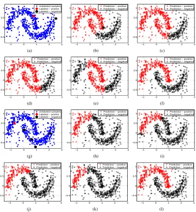
Figure 3: Examples illustrating the sensitivity of graph-based SSLto adverse labeling conditions.

Particularly challenging conditions are shown in (a) where an uninformative label on an outlier sample is the only negative label (denoted by a black circle) and in (g) where

imbalanced labeling is involved. Prediction results are shown for theGFHFmethod (Zhu

et al., 2003) in (b) and (h), theLGCmethod (Zhou et al., 2004) in (c) and (i), theLapSVM

method (Belkin et al., 2006) in (d) and (j), theTSVMmethod (Joachims, 1999) in (e) and

(k); and our method in (f) and (l).

the graph is perfectly constructed from the data, problematic initial labels under practical situations

can easily deteriorate the performance of SSL prediction. Figure 3 provides examples depicting

negative label (dark circle) is located in an outlier region where the low density connectivity limits

its diffusion to the rest of the graph. The leading SSLmethods classify the majority of unlabeled

nodes in the graph as positive (Figure 3(b)-Figure 3(e)). Such conditions are frequent in real prob-lems like content-based image retrieval (CBIR) where the visual query example is not necessarily representative of the class. Another difficult case is due to imbalanced labeling. There, the ratio of training labels is disproportionate to the underlying class proportions. For example, Figure 3(g) depicts two half-circles with an almost equal number of samples. However, since the training labels

contain three negative samples and only one positive example, theSSLpredictions are strongly

bi-ased towards the negative class (see Figures 3(h) to 3(k)). This imbalanced labeling situation occurs frequently in realistic problems such as the annotation of microscopic images (Wang et al., 2008a). Therein, the human labeler favors certain cellular phenotypes due to domain-specific biological

hy-potheses. To tackle these issues, we next propose a novel bivariate framework for graph-basedSSL

and describe an efficient algorithm that achieves it via alternating minimization.

3. Bivariate Framework for Graph-BasedSSL

We first propose an extension to the existing graph regularization-basedSSLformulations by casting

the problem as abivariateoptimization over both the classification function and the unknown labels.

Then we demonstrate that the minimization of this bivariate cost reduces to a linearly constrained binary integer programming (BIP) problem. This problem can be approximated via semi-definite programming yet this approach is impractical due to scalability issues. We instead explore a fast method which alternates minimization of the cost over the label matrix and the prediction function.

3.1 The Cost Function

Recall the univariate regularization formulation for graph-basedSSLin Equation (3). Also note that

the optimization problem in existing approaches such as LGC andGFHFcan be broken up into

separate parallel problems since the cost function decomposes into additive terms that only depend

on individual columns of the prediction matrixF(Wang et al., 2008a). Such a decomposition reveals

that biases may arise if the input labels are disproportionately imbalanced. In addition, when the graph contains background noise and makes class manifolds non-separable (as in Figure 1(b)), these existing graph transduction approaches fail to output reasonable classification results.

Since the univariate framework treats the initial label information as a constant, we propose a novel bivariate optimization framework that explicitly optimizes over both the classification function

Fand the binary label matrixY:

(F∗,Y∗) =arg min_F∈Rn×c_,Y∈Bn×c

Q

(F,Y)

s.t. yi j ∈ {0,1},

∑

cj=1yi j=1,

yi j=1, for zi= j, j=1,···,c.,

where_Bn×c _{is the set of all binary matricesYof sizen×c. For a labeled samplex}

i ∈Xl,yi j =1

ifzi = j, and the constraint∑cj=1yi j =1 indicates that this a single label prediction problem. We

specify the cost function as

Q

(F,Y) =1

2tr

Finally, rewriting the cost as a summation (Zhou et al., 2004) reveals a more intuitive formulation where

Q

(F,Y) =1

2

n

∑

i=1 n

∑

j=1

wi j

Fi· √

di − Fj·

p

dj

2

+µ

2

n

∑

i=1

kFi·−Yi·k2.

3.2 Reduction to a Univariate Problem

In the new graph regularization framework proposed above, the cost function involves two variables to be optimized. Simultaneously recovering both solutions is intractable due to the mixed integer

programming problem over binary Yand continuousF. To solve the issue, we first show how to

reduce the original mixed problem to a univariate optimization problem with respect to the label

variableY.

Foptimization step:

In each loop withYfixed, the classification functionF_∈Rn×c is continuous and the cost function

is convex, allowing the minimum to be recovered by setting the partial derivative to zero:

∂

Q

∂F∗ =0=⇒LF

∗_+µ(F∗_{−Y) =0}

=_⇒F∗= (L/µ+I)−1Y=PY, (7)

where we denote thePmatrix as

P= (L/µ+I)−1_,

and name it thepropagation matrixsince it is used to derived a prediction functionFgiven a label

matrixY. Because the graph is often symmetric, it is easy to show that the graph LaplacianLand

the propagation matrixPare both symmetric.

Yoptimization step:

Next replaceFin Equation (6) by its optimal valueF∗from the solution of Equation (7). This yields

Q

(Y) = 1

2tr(Y

⊤_P⊤_{LPY+µ(PY−Y)}⊤_(PY−Y))

= 1

2tr

Y⊤

h

P⊤LP+µ(P⊤₋I)(P₋I)iY

=1

2tr

Y⊤AY

,

where we group all the constant parts in the above equation and define

A=P⊤LP+µ(P⊤₋I)(P₋I) =P⊤LP+µ(P₋I)2.

The final optimization problem becomes

Y∗=arg min1

2tr

Y⊤AY

s.t. yi j∈ {0,1},

∑

jyi j=1, j=1,···,c

The first constraint produces a binary integer problem and the second one ∑jyi j =1 produces a

single assignment constraint, that is, each vertex can only be assigned one class label. The third

group of constraints encodes the initial label information in the variableY. Since the binary matrix

Y_∈Bn×c _{is subject to linear constraints of the form∑}

jyi j=1 and initial labeling conditions, the

optimization in Equation (8) requires solving a linearly constrained binary integer programming (BIP) problem which is NP hard (Cook, 1971; Karp, 1972).

3.3 Incorporating Label Normalization

A straightforward approach to solving the minimization problem in Equation (8) is to use the

gradi-ent to greedily update the label variableY. However, this may produce biased classification results

in practice since, at each iteration, the class with more labels will be preferred and will propagate more quickly to the unlabeled examples. This arises in practice (as in Figure 3) and is due to the

fact thatYstarts off sparse and contains many unknown entries. To compensate for this bias during

label propagation, we propose using a normalized label variable ˜Y=ΛΛΛY for computing the cost

function in Equation (6) as

Q

= 1

2tr

F⊤LF+µ(F₋Y˜)⊤(F₋Y˜)

= 1

2tr

F⊤LF+µ(F₋ΛΛΛY)⊤(F₋ΛΛΛY). (9)

The diagonal matrixΛΛΛ=diag(λλλ) =diag([λ1,···,λn])is introduced to re-weight or re-balance the

influence of labels from different classes as it modulates the label importance based on node degree.

The value ofλi (i=1,···,n) is computed using the vertex degreedi and label information

λi=

(

pj·_∑kd_{yk j}i _dk : yi j=1

0 : otherwise, (10)

where pj is the prior of class jand is subject to the constraint

c

∑

j=1

pj=1. The value of pj can be

either estimated from the labeled training set or simply set to be uniform pj=1/c(j=1, ···, c)

in agnostic situations (when no better prior is available or if the labeled data is plagued by biased

sampling). Using the normalized label matrix ˜Yin the bivariate formulation allows labeled nodes

with high degrees to contribute more during the label propagation process. However, the total diffusion of each class is kept equal (for agnostic settings with no priors available) or proportional to the class prior (for the setting with prior information). Therefore, the influence of different classes is balanced even if the given class labels are imbalanced. If class proportion information is known, it can be integrated by scaling the diffusion with the appropriate prior. In other words, the label

normalization attempts to enforce simple concentration inequalities which, in theiidcase require

the predicted label results to concentrate around the underlying class ratios (Huang and Jebara, 2010). This intuition is in line with prior work that uses class proportion information in transductive inference where class proportion is enforced as a hard constraint (Chapelle et al., 2007) or as a regularizer (Mann and McCallum, 2007).

3.4 Alternating Minimization Procedure

obtain the optimal solutionF∗and the final cost function with respect to label variableYas

F∗=PY˜ =PΛΛΛY, (11)

Q

=1

2tr

˜

Y⊤AY˜=1

2tr

Y⊤ΛΛΛAΛΛΛY. (12)

Instead of finding the global optimumY∗, we only take an incremental step in each iteration to

modify a single entry in Y. Namely in each iteration, we find the optimal position (i∗,j∗) in the

matrixYand change the binary value ofyi∗_j∗from 0 to 1. To do this, we find the direction with the

largest negative gradient guiding our choice of binary step onY. Specifically, we evaluate_{k ▽}

Q

Yk

and find the largest negative value to determine(i∗,j∗).

Note that the settingyi∗_j∗=1 is equivalent to modifying the normalized label matrix ˜Yby setting

˜

yi∗_,j∗=ε_i∗,0<ε_i∗<1, andY,Y˜ can be converted from each other componentwise. Thus, the greedy

optimization of

Q

with respect toYis equivalent to greedy minimization of

Q

with respect to ˜Y.

More formally, we derive the gradient of the above loss function∇Y˜

Q

= ∂_∂Q_Y˜ and recover it with

respect toYas:

∂

Q

∂Y˜ =A

˜

Y=AΛΛΛY. (13)

As described earlier, we search the gradient matrix∇_Y˜

Q

to find the minimal element

(i∗,j∗) =arg min_{xi∈Xu,1≤j≤c}∇y˜i j

Q

.

Because of the binary nature of Y, we simply set yi∗_j∗ =1 instead of making a continuous

update. Accordingly, the node weight matrixΛΛΛt+1 can be recalculated with the updatedYt+1 in

the iterationt+1. The update ofYis greedy and thus it could backtrack from predicted labels in

previous iterations without convergence guarantees. We propose a straightforward way to guarantee convergence and avoid backtracking or unstable oscillation in the greedy propagation process: once an unlabeled point has been labeled, its labeling can no longer be changed. Thus, we remove the

most recently labeled point(i∗,j∗)from future consideration and conduct search over the remaining

unlabeled data only. In other words, to avoid retroactively changing predicted labels, the labeled

vertexxi∗ is removed fromX_uand added toX_l.

Note that although the optimalF∗can be computed using Equation (11), this need not be done

explicitly. Instead, the new value is implicitly used in Equation (14) only to updateY. In the

fol-lowing, we summarize the update rules from stepttot+1 in the alternating minimization scheme.

. Compute gradient matrix:

(∇_Y˜

Q

)t = AY˜t=AΛΛΛtYt,ΛΛΛt =diag(λλλt).

. Update one label:

(i∗,j∗) = arg min_{xi∈Xu,1≤j≤c}(∇y˜i j

Q

)

t_,

. Update label normalization matrix:

λt+1 =

( _Dii

∑kYtk j+1Dkk : y

t+1 i j =1

0 : otherwise.

. Update the list of labeled and unlabeled data:

Xt_l+1_←−Xt_l+xi∗ ; Xt_u+1←−Xt_u−x_i∗.

Starting with a few given labels, the method iteratively and greedily updates the label matrixY

to derive new labels in each iteration. The newly obtained labels are then use in the next iteration. Notice that the label normalization vector is re-computed for each iteration due to the change of label set. Although the original objective is formed in a bivariate manner in Equation 6, the above alternating optimization procedure drives the prediction of new labels without explicitly calculating

F∗as is done in other graph transduction methods likeLGCandGFHF. This unique feature makes

the proposed algorithm very efficient since we only update the gradient matrix∇Y˜

Q

for prediction

new labels in each iteration.

Due to the greedy assignment step and the lack of back-tracking, the algorithm can repeat the

alternating minimization (or the gradient computation) at most n₋l times. Each minimization

step overF andYrequires

O

(n2)complexity and, thus, the total complexity of the above greedy

algorithm is

O

(n3). However, the update of the graph gradient can be done efficiently by modifying

only a single entry inYper iteration. This further reduces the computational cost down to

O

(n2).

Empirically, the value of the loss function

Q

decreases rapidly in the the first dozen iterations and

steadily converges afterward (Wang et al., 2009). This phenomenon indicates that early stopping strategy could be applied to speed up the training and prediction (Melacci and Belkin, 2011). Once the first few iterations are completed, the new labels are added and the standard propagation step can

be used to predict the optimalF∗as indicated in Equation (11) over the whole graph in one step. The

details of the algorithm, namelygraph transduction via alternating minimization, can be referred to

Wang et al. (2008b). In the following section, we provide a greedy Max-Cut based solution, which essentially interprets the above alternating minimization procedure from a graph cut view.

4. Greedy Max-Cut for Semi-Supervised Learning

In this section, we introduce a connection between the proposed bivariate graph transduction frame-work and the well-known maximum cut problem. Then, a greedy gradient based Max-Cut solution will be developed and related to the above alternating minimization algorithm.

4.1 Equivalence to a Constrained Max-Cut Problem

Recall the optimization problem defined in Equation (8) which is exactly a linearly constrained binary integer programming (BIP) problem. In the case of a two-class problem, this optimization

will be reduced to a weighted Max-Cut problem over the graph

G

A = {X,A} subject to linear

constraints. The cost function in Equation (8) can be rewritten as

Q

(Y) =1

2tr

Y⊤AY

=1

2tr

AYY⊤

=1

whereA=_{ai j}andR=YY⊤. Considering the constraints∑jyi j=1 andY∈Bn×2for a two-class

problem, we let

Y= [y e₋y],

wherey_∈Bn_(i.e.,y={y

i},yi∈ {0,1},i=1,···,n)ande= [1,1,···,1]⊤are column vectors. Then

rewriteRas

R = YY⊤= [y e₋y][y e₋y]⊤

= ee⊤₋y(e⊤₋y⊤)₋(e₋y)y⊤. (14)

Now rewrite the cost function in Equation (14) by replacingRwith Equation (14)

Q

(y) =1

2tr

Ahee⊤₋y(e⊤₋y⊤)₋(e₋y)y⊤i.

Sinceee⊤is the all-ones matrix, we obtain

1 2tr

Aee⊤=1

2

∑

_i

∑

_j Ai j.

It is easy to show thatAis symmetric and

y(e⊤₋y⊤) = [(e₋y)y⊤]⊤.

Next, simplify the cost function

Q

as

Q

(y) = 1

2tr

Aee⊤

−tr

h

(e⊤₋y⊤)Ay

i

= 1

2tr

Aee⊤

−y⊤A(e₋y).

Since the first part is a constant, the optimal value y∗ of the above minimization problem is the

argument of the maximization problem

y∗=arg min

y

Q

(y) =arg maxy y

⊤_A(e−y).

Define a new function f(y)as

f(y) =y⊤A(e₋y).

Again, the variable y_∈Bn _{is a binary vector and e = [1,1,···,1]}⊤ _{is the unit column vector.}

Now we show that maximization of the above function maxyf(y)is exactly a Max-Cut problem if

we treat the symmetric matrixAas the weighted adjacency matrix of an undirected graph

G

A=

{VA,A}. Note that the diagonal elements of A could be non-zeroAii6=0,i=1,2,···,n, which

indicates the undirected graph

G

A has self-connected nodes. Assume A=A0+AΛ, where A0

is the matrix obtained by zeroing the diagonal elements of Aand AΛ is a diagonal matrix with

AΛ_ii =Aii,AΛi j=0,i,j = 1,2,···,n,i6= j. It is straightforward to show that the the function f(y)

can be written as

In other words, the non-zero elements inAdo not affect the value of f(y). Therefore, in the rest

of this article, we can assume that the matrixAhas zero diagonal elements unless the text specifies

otherwise.

Sincey=_{y1,y2,···,yn}is a binary vector, each setting ofypartitions the vertex setVAin the

graph

G

Ainto two disjoint subsets(S1,S2). In other words, the two subsetsS1={vi|yi=1}and

S2={vi|yi=0}satisfyS1∪S2=VAandS1∩S2=/0. The maximization problem can then be written

as

maxf(y) =max

∑

i,j

ai j·yi(1−yj) =max

1

2_v

∑

i∈S1

vj∈S2 ai j.

Because each binary vectoryresulting in a partition(S1,S2)over the graph

G

Aand f(y)is a

corre-spondingcut, the above maximization maxf(y)is easily recognized as a Max-Cut problem (Deza

and Laurent, 2009). However, in graph based semi-supervised learning, the variabley is partially

specified by the initial label values. This given label information can be interpreted as a set of linear constraints on the Max-Cut problem. Thus, the optimal solution can achieved by solving a linearly constrained Max-Cut problem (Karp, 1972). In addition, we also show that a multi-class problem

equals a MaxK-Cut problem (K=c) (refer to Appendix A). Note that previous work used min-cut

over the original data graph

G

=_{X,W_}to perform semi-supervised learning (Blum and Chawla,

2001; Blum et al., 2004). A key difference of the above formulation lies in the fact that we perform

max-cut over the transformed graph

G

A = {X,A}.

However, since there is no guarantee that the weights on the graph

G

A are non-negative,

so-lutions to the Max-Cut problem can be difficult to find (Barahona et al., 1988). Therefore, in the following subsection, we will propose a gradient greedy solution to efficiently solve the above Max-Cut problem, which can be treated as a different view of the previous alternating minimization solution.

4.2 Label Propagation by Gradient Greedy Max-Cut

For the standard Max-Cut problem, many approximation techniques have been developed, including the most remarkable Goemans-Williamson algorithm using semidefinite programming (Goemans and Williamson, 1994, 1995). However, applying these guaranteed approximation schemes to solve

the constrained Max-Cut problem forY mentioned above is infeasible due to the constraints on

initial labels. Furthermore, there is no guarantee that all edge weights ai j of the graph

G

A are

non-negative, a fundamental requirement in solving a standard Max-Cut problem (Goemans and Williamson, 1995). Instead, here we use a greedy gradient based strategy to find local optima by assigning each unlabeled vertex to the label set with minimum connectivity to maximize cross-set edge weights iteratively.

The greedy Max-Cut algorithm randomly selects unlabeled vertices and places each of them into the appropriate class subset depending on the edges between this unlabeled vertex and the vertices

in the labeled subset. Given the label information, the initial label set for class jcan be constructed

as

S

j={xi|yi j=1}or

S

j ={xi|zi= j},i=1,2,···,n;j=1,2,···,c. Define the following as the

connectivity between unlabeled vertexxiand labeled subset

S

j

ci j= n

∑

m=1

Algorithm 1Greedy Max-Cut for Label Propagation

Input:the graph

G

A={X,A}, the given labeled vertexXl, and initial labelsY; Initialization:

obtain the initial cut_{

S

j}by assigning the labeled vertexXl to each subset:

S

j={xi|yi j=1},j=1,2,···,c

unlabeled vertex setXu=X\Xl;

repeat

randomly select an unlabeled vertexxi∈Xu

compute the connectivityci j,j=1,2,···,c

place the vertex to the labeled subject

S

j∗:

j∗=arg minjci j

addxitoXl:Xl←−Xl+xi;

removexifromXu:Xu←−Xu−xi;

until Xu= /0

Output: the final cut and the corresponding labeled subsets

S

j,j=1,2,···,c

whereAi.is thei’th row vector ofAandY.jis the j’th column vector ofY. Intuitively,ci jrepresents

the sum of edge weights between vertexxiand label set

S

jgiven the graph

G

Awith edge weightsA.

Based on this definition, a straightforward local search for the maximum cut involves placing each

unlabeled vertexxi ∈Xuin the labeled subset

S

j with minimum connectivity ci j to maximize the

cross-set edge weights as shown in Algorithm (1). In order to achieve a good solution Algorithm (1) should be run multiple times with different random seeds after which the best cut overall is output (Mathieu and Schudy, 2008).

While the above method is computationally cumbersome, it still does not resolve the issue of undesired local optima and may generate biased cuts. According to the definition in Equation (15), the initialized labels determine the connectivity between unlabeled vertices and labeled subsets. If the computed connectivity is negative, the above random search will prefer assigning unlabeled vertices to the label set with the most labeled vertices which results in biased partitioning. Such biased partitioning also occurs in minimum cut problems over an undirected graph with positive weights (Shi and Malik, 2000). Other label initialization problems may also produce a poor cut. For example, the numbers of labels from different classes may deviate from the underlying class proportions. Alternatively, the labeled vertices may be outliers and lie in regions of the graph with low density. Such labels often lead to weak label prediction results (Wang et al., 2008a). Furthermore, the algorithm’s random selection of an unlabeled vertex results in unstable predictions

since the chosen unlabeled vertexxi could have equally low connectivity to multiple label subsets

S

j.

To address the aforementioned issues, we first modify the original definition of connectivity to alleviate label imbalance across different classes. A weighted connectivity is computed as

ci j=pj· n

∑

m=1

λmaimym j=pj·ΛΛΛAi.Y.j. (16)

The diagonal matrixΛΛΛ=diag([λ1,λ2, ···, λn]is called the label weight matrix as in Equation (10)

λi=

di/dSj : if xi∈

S

j,j=1,···,c

Algorithm 2Greedy Gradient based Max-Cut for Label Propagation

Input:the graph

G

A={X,A}and the given labeled vertexXl, and initial labelY; Initialization:

obtain the initial cut_{

S

j}through assigning the labeled vertexXlto each subset:

S

j={xi|yi j=1},j=1,2,···,c

unlabeled vertex setXu=X\Xl;

repeat

for all j=0 to_|Xu|do

compute weighted connectivity:

ci j= n

∑

k=1

λiaikyk j,xi∈Xu,j=1,···,c

end for

update the cut_{

S

i}by placing the vertexxi∗ to the

S

_j∗’th subset:

(i∗,j∗) =arg min

i,j,xi∈Xu

ci j

addxitoXl:Xl←−Xl+xi;

removexifromXu:Xu←−Xu−xi;

until Xu= /0

Output: the final cut and the corresponding labeled subsets

S

j,j=1,2,···,c

wheredSj =∑xm∈Sjdmis the sum of the degrees of the vertices in the label set

S

j. This heuristic

setting weights the importance of each label based on degree which alleviates the adverse impact of

outliers. If we ignore class priors, this definition ofΛΛΛcoincides with the one in Equation (10).

Finally, to handle any instability due to the random search algorithm, we propose a greedy gradient search approach where the most beneficial vertex is assigned to the label set with minimum

connectivity. In other words, we first compute the connectivity matrixC=_{ci j} ∈Rn×cthat gives

the connectivity between all unlabeled vertices to existing label sets

C=AΛΛΛY.

Then we examineCto identify the element(i∗,j∗)with minimum value as

(i∗,j∗) =arg min

i,j:xi∈Xu

ci j.

This means that the unlabeled vertex xi∗ has the least connectivity with label set

S

_j∗. Then, we

update the labeled set

S

j∗ by adding vertexx_i∗ as one greedy step to maximize the cross-set edge

weights. This greedy search can be repeated until all the unlabeled vertices are assigned to labeled sets. In each iteration of the greedy cut process, the weighted connectivity of all unlabeled vertices to labeled sets is re-computed. Then the vertex with minimum connectivity is placed in the proper labeled set. The algorithm is summarized in Algorithm (2).

The connectivity matrix Ccan also be viewed as the gradient of the cost function

Q

in

Equa-tion (12) with respect to ˜Y. This is precisely the same setting used in Equation (13) of the alternating

minimization algorithm

C=∂

Q

We name the algorithm greedy gradient Max-Cut (GGMC) since, in the greedy step, the

unla-beled vertices are assigned labels in a manner that reduces the value of

Q

along the direction of

the steepest descent. Consider both the variablesYandFin the original bivariate formulation in

Equation (9). The greedy Max-Cut method is equivalent to the alternating minimization procedure

discussed earlier. Unlike graph-cut basedSSLmethods such as mincuts (Blum and Chawla, 2001;

Blum et al., 2004), ourGGMCalgorithm tends to generate more natural graph cuts and avoid biased

solutions since it uses a weighted connectivity matrix. This allows it to effectively handle the issues mentioned earlier and, in practice, achieve significant gains in accuracy while retaining efficiency.

4.3 Complexity and Speed Up

Assume the graph hasn=_|X_|vertices and a subsetXl withl=|Xl|labeled vertices (wherel≪n).

The greedy gradient algorithm terminates after at most n₋l_≃n iterations. In each iteration of

the greedy gradient algorithm, the connectivity matrixCis updated by a matrix multiplication (an

n_×n-matrix is multiplied by a n_×c-matrix). Hence, the complexity of the greedy algorithm is

O

(cn3).

However, the greedy algorithm can be greatly accelerated in practice. For example, the com-putation of the connectivity in Equation (16) can be done incrementally after assigning each new unlabeled vertex to a certain label set. This circumvents the re-calculation of all the entries in the

Cmatrix. Assume in thet’th iteration the connectivity isCt and an unlabeled vertexxiwith degree

di is assigned to the labeled set

S

j. Clearly, for all remaining unlabeled vertices, the connectivity

to the labeled sets remains unchanged except for the j’th labeled set. In other words, only the j’th

column ofCneeds updating. This update is performed incrementally via

Ct_.+_j1= dS

t j

d_St+1

j

Ct_.j+ di

d_St+1

j

A.i,

whered_St+1

j =dS t

j+diis the sum of the degrees of the labeled vertices after assigningxito the labeled

set

S

j. This incremental update reduces the complexity of the greedy gradient search algorithm to

O

(n2).

5. Experiments

In this section, we demonstrate the superiority of the proposedGGMCmethod over state-of-the-art

semi-supervised learning methods using both synthetic and real data. Previous work showed that LapSVM andLapRLS outperform other semi-supervised approaches such as Transductive SVMs

TSVM(Joachims, 1999) and∇TSVM(Chapelle and Zien, 2005). Therefore, we limit our

compar-isons to only theLapRLS,LapSVM(Sindhwani et al., 2005; Belkin et al., 2005),LGC(Zhou et al.,

2004) andGFHF(Zhu et al., 2003). To set various hyper-parameters such asγI,γr inLapRLSand

LapSVM, we followed the default configurations used in the literature. Similarly, forGGMCand

LGC, we set the hyper-parameterµ=0.01 across all data sets. For the computational cost,GGMC,

LGC and GFHF required very similar run-times to output a prediction. However, LapRLS and

LapSVMneed significant longer training time, especially for multiple-class problems since multiple rounds of one-vs-all training have to be performed.

As in Section 2, any real implementation of graph-basedSSLneeds a graph construction method

2 3 4 5 6 7 8 9 10 0

0.1 0.2 0.3

The number of labels

Error Rate LGC GFHF LapSVM LapRLS GGMC (a)

2 3 4 5 6 7 8 9 10 0

0.1 0.2 0.3

The number of labels

Error Rate LGC GFHF LapSVM LapRLS GGMC (b)

2 3 4 5 6 7 8 9 10 0

0.1 0.2 0.3

The number of labels

Error Rate LGC GFHF LapSVM LapRLS GGMC (c)

4 5 6 8 10 12 14 16 18 20 0

0.1 0.2 0.3 0.4

The number of neighborhoods

Error Rate LGC GFHF LapSVM LapRLS GGMC (d)

4 5 6 8 10 12 14 16 18 20 0

0.1 0.2 0.3

The number of neighborhoods

Error Rate LGC GFHF LapSVM LapRLS GGMC (e)

4 5 6 8 10 12 14 16 18 20 0

0.1 0.2 0.3 0.4

The number of neighborhoods

Error Rate LGC GFHF LapSVM LapRLS GGMC (f)

1 2 4 6 8 10 12 14 16 18 20 0 0.1 0.2 0.3 0.4 0.5 Imbalance Ratio Error Rate LGC GFHF LapSVM LapRLS GGMC (g)

1 2 4 6 8 10 12 14 16 18 20 0 0.1 0.2 0.3 0.4 0.5 Imbalance Ratio Error Rate LGC GFHF LapSVM LapRLS GGMC (h)

1 2 4 6 8 10 12 14 16 18 20

0 0.1 0.2 0.3 0.4 0.5 Imbalance Ratio Error Rate LGC GFHF LapSVM LapRLS GGMC (i)

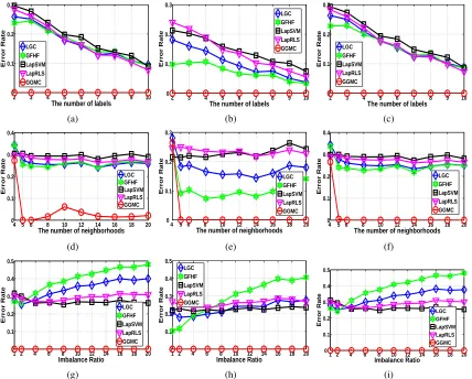
Figure 4: Experimental results on the noisy two-moon data set simulating different graph construc-tion approaches and label condiconstruc-tions. Figures a) d) g) use binary weighting. Figures b) e) h) use fixed Gaussian kernel weighting. Figures c) f) i) use adaptive Gaussian kernel

weighting. Figures a) b) c) vary the number of labels. Figures d) e) f) vary the value ofk

in the graph construction. Figures g) h) i) vary the label imbalance ratio.

procedure to generate the sparse connectivity matrixBand a weighting procedure to obtain weights

on the edges inB. In these experiments, we used the same graph construction procedure for all the

SSLalgorithms. The sparsification was done using the standardk-nearest-neighbors approach and

the edge weighting involved eitherbinary weightingorGaussian kernel weighting. In the latter case,

theℓ2distancedℓ2(xi,xj)is used and the kernel bandwidthσis estimated in two different ways. The

first estimate uses a fixedσdefined as the average distance between each selected sample and itsk’th

nearest neighbor (Chapelle et al., 2006). In addition, a second adaptive approach is also considered

which locally estimates the parameterσto the mean distance in thek-nearest neighborhoods of the

20 30 40 50 60 70 80 90 100 0

0.05 0.1 0.15 0.2 0.25

The number of labels

Error Rate

LGC GFHF LapSVM LapRLS GGMC

(a)

20 30 40 50 60 70 80 90 100 0

0.05 0.1 0.15 0.2 0.25

The number of labels

Error Rate

LGC GFHF LapSVM LapRLS GGMC

(b)

20 30 40 50 60 70 80 90 100 0

0.05 0.1 0.15 0.2 0.25

The number of labels

Error Rate

LGC GFHF LapSVM LapRLS GGMC

(c)

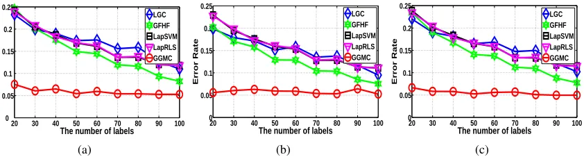
Figure 5: Experimental results on the USPS digits data set under varying levels of labeling using: a) binary weighting; b) fixed Gaussian kernel weighting and c) adaptive Gaussian kernel weighting.

5.1 Noisy Two-Moon Data Set

We first compared GGMC with several representative SSL algorithms using the noisy two-moon

data set shown in Figure 3. Despite the near-perfect classification results reported on clean versions of this data set (Sindhwani et al., 2005; Zhou et al., 2004), small amounts of noise quickly degrade the performance of previous algorithms. In Figure 3, two separable manifolds containing 600 two-dimensional points are mixed with 100 noisy outlier samples. The noise foils previous methods which are sensitive to the locations of the initial labels, disproportional sampling from the classes, and outlier noise. All experiments are repeated with 100 independent folds with random sampling to show the average error rate of each algorithm.

The first group of experiments varies the number of labels provided to the algorithms. We

uniformly usedk=6 in thek-nearest-neighbors graph construction and applied the aforementioned

three edge-weighting schemes. The average error rates of the predictions on the unlabeled points is shown in Figures 4(a), 4(b) and 4(c). These correspond to binary edge weighting, fixed Gaussian kernel edge weighting, and adaptive Gaussian kernel edge weighting, respectively. The results

clearly show thatGGMCis robust to the size of the label set and and generates perfect prediction

results for all three edge-weighting schemes.

The second group of experiments demonstrate the influence of the number of edges (i.e., the

value ofk) in the graph construction method. We varied the value ofkfrom 4 to 20 and Figures 4(d),

4(e), and 4(f) show results for the different edge-weighting schemes. Once again,GGMCachieves

significantly better performance in most cases.

Finally, we studied the effect of imbalanced labeling on theSSL algorithms. We fix one class

to have only one label and then randomly selectr labels from the other classes. Here,r indicates

the imbalance ratio and we study the range 1_≤ r _≤20. Figures 4(g), 4(h), and 4(i) show the

results with different edge-weighting schemes. Clearly,GGMCis insensitive to the imbalance since

it computes a per-class label weight normalization which compensates directly for differences in label proportions.

In summary, Figure 4 depicted the performance advantages ofGGMCrelative toLGC,GFHF,

LapRLS, andLapSVMmethods. We clearly see that the four previous algorithms are sensitive to the initial labeling conditions and none of them produces perfect prediction. Furthermore, the error

6 9 12 15 18 21 24 27 30 0 0.05 0.1 0.15 0.2

The number of labels

Error Rate LGC GFHF LapSVM LapRLS GGMC (a)

6 9 12 15 18 21 24 27 30 0

0.05 0.15 0.25 0.35

The number of labels

Error Rate LGC GFHF LapSVM LapRLS GGMC (b)

4 6 8 10 12 14 16 18 20 0

0.05 0.15 0.25

The number of labels

Error Rate LGC GFHF LapSVM LapRLS GGMC (c)

6 9 12 15 18 21 24 27 30 0

0.05 0.1 0.15 0.2

The number of labels

Error Rate LGC HFGF LapSVM LapRLS GGMC (d)

6 9 12 15 18 21 24 27 30

0 0.05 0.1 0.15 0.2 0.25

The number of labels

Error Rate LGC HFGF LapSVM LapRLS GGMC (e)

4 6 8 10 12 14 16 18 20 0.05

0.1 0.15 0.2 0.25

The number of labels

Error Rate LGC HFGF LapSVM LapRLS GGMC (f)

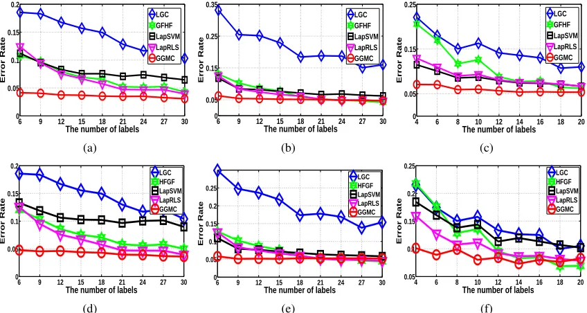
Figure 6: Performance ofLGC,GFHF,LapRLS,LapSVM, andGGMCalgorithms using the UCI

data sets. The horizontal axis is the number of training labels provided while the vertical

axis is the average error rate achieved over 100 random folds. Results are based onk

-nearest neighbor graphs shown in a) for the Iris data set, in b) for the Wine data set and

in c) for the Breast Cancer data set. Results are based onb-matched graphs shown in d)

for the Iris data set, in e) for the Wine data set and in f) for the Breast Cancer data set.

labels are made available. However, GGMC achieves high accuracy regardless of the imbalance

ratio and the size of the label set. Furthermore, GGMCremains robust to the graph construction

procedure and the edge-weighting strategy.

5.2 Handwritten Digit Data Set

We also evaluated the algorithms in an image recognition task where handwritten digits in the USPS

database are to be annotated with the appropriate label_{0,1, . . . ,9_}. The data set contains gray scale

handwritten digit images involving 16_×16 pixels. We randomly sampled a subset of 4000 samples

from the data. For all the constructed graphs, we used thek-nearest-neighbors algorithm withk=6

and tried the three different edge-weighting schemes above. We varied the total number of labels from 20 to 100 while guaranteeing that each digit class had at least one label. For each setting, the average error rate was computed over 20 random folds.

The experimental results are shown in Figures 5(a), 5(b), and 5(c) which correspond to the three

different edge-weighting schemes. As usual,GGMCsignificantly improves classification accuracy

relative to other approaches, especially when few labeled training examples are available. The

average error rates ofGGMCare consistently low with small standard deviations. This demonstrates