Linear Programs for Hypotheses Selection in
Probabilistic Inference Models
Anders Bergkvist [email protected]
Department of Molecular Biology G¨oteborg University
P.O. Box 462
40530 G¨oteborg, Sweden
Peter Damaschke [email protected]
Department of Computer Science and Engineering Chalmers University
41296 G¨oteborg, Sweden
Marcel L ¨uthi [email protected]
Department of Computer Science University of Basel
4056 Basel, Switzerland
Editors: Kristin P. Bennett and Emilio Parrado-Hern´andez
Abstract
We consider an optimization problem in probabilistic inference: Given n hypotheses Hj, m possi-ble observations Ok, their conditional probabilities pk j, and a particular Ok, select a possibly small subset of hypotheses excluding the true target only with some error probabilityε. After specifying the optimization goal we show that this problem can be solved through a linear program in mn vari-ables that indicate the probabilities to discard a hypothesis given an observation. Moreover, we can compute optimal strategies where only O(m+n)of these variables get fractional values. The man-ageable size of the linear programs and the mostly deterministic shape of optimal strategies makes the method practicable. We interpret the dual variables as worst-case distributions of hypotheses, and we point out some counterintuitive nonmonotonic behaviour of the variables as a function of the error boundε. One of the open problems is the existence of a purely combinatorial algorithm that is faster than generic linear programming.
Keywords: probabilistic inference, error probability, linear programming, cycle-free graphs,
net-work flows
1. Introduction
Suppose that we are given one of m possible observations Ok, k=1, . . . ,m, and n hypotheses Hj, j=1, . . . ,n, each of which might have caused the observed Ok. Moreover we know the conditional probabilities pk j=P(Ok|Hj)to observe Okif Hjis the true hypothesis, also called the target. Since exactly one Ok is observed, the pk jmust satisfy∑mk=1pk j=1 for every j. The pk jmay come from background knowledge of causal relations, or they may be estimated from statistical data.
then examined closer, in order to identify the target, whereas we would come back to discarded hypotheses only if we missed the target in our selection. In Section 2 we will state this problem formally as an optimization problem, namely, the minimization of the expected weight of excluded hypotheses, given an error probability bound for each target. We think that the problem is very fundamental and its optimization view could be interesting for any setting where one has to guess hypotheses from data with known conditional distributions.
An obvious application scenario is diagnosis. The probabilities of various syndromes caused by any disease may be known from a database. In each particular case with a given syndrome, one wants to narrow down the set of suspects, that is, of possible diseases to be examined more carefully. But the true hypothesis should, with high probability, not be discarded in the beginning. See the discussion by Szolovits et al. (1988) which refers, however, to complex and structured models rather than “atomic” hypotheses and data.
Our particular motivation however came from a protein structure prediction project. Proteins are sequences of residues, each residue being derived from one of 20 possible amino acids. The 3D structure of the protein backbone is uniquely determined by its torsion angles. Since it is dif-ficult and costly to determine them experimentally, various methods have been developed to infer torsion angles and other structure elements from easier measurable, correlated data, partly with help of sequence homology. Nuclear magnetic resonance (NMR) chemical shifts of nuclei in the amino acids are certain spectroscopic data influenced by the local molecular conformation, see Beger and Bolton (1997); Cornilescu et al. (1999); Wang and Jardetzky (2002); Xu and Case (2002) for more background information. Due to the correlations, it is a natural idea to infer torsion angles from measured chemical shifts. Torsion angle restraints that are narrow but still contain the (unknown) true torsion angle values in the majority of cases are important for correct 3D structure reconstruc-tion of whole protein sequences. Since the correlareconstruc-tions are complicated and can hardly be put in a neat formula, we have chosen a statistical approach based on large samples of data. That is, the “local” task of predicting single torsion angle restraints leads to instances of the optimization prob-lem as considered here: Our hypotheses are torsion angles, our observations are measured chemical shifts, both discretized in finitely many intervals, and the pk j are estimated from a database. Our raw data are scatterplots of chemical shift vs. torsion angle values from public databases. The dis-cretization is done in a preprocessing phase, with the aim to partition the scatterplot into a coarse grid where the data points in each rectangle are approximately evenly distributed (so that further splitting would be meaningless). The current partitioning heuristic is described by Christin (2006). Then, we apply different prediction heuristics to the discretized scatterplots, that is, point count matrices. The role of optimization in this application is discussed after the main part of the paper, in Section 7. We have to treat in a semi-automated way a huge number of problem instances: for 6 different nuclei, 20 different amino acids, and 2 torsion angles we get nearly 240 data sets. (A few are empty.) Actually, the number of instances is a multiple of this number when we consider several error probability bounds and their combinations, maybe several discretizations, different sources of raw data, etc. In this sense our application is large-scale, even though the single problem instances are not. On the contrary, we need to reduce every instance to some efficiently solvable optimization problem in order to keep the project feasible. In this paper we will show several beneficial properties of the optimization problem that comply with this goal:
possi-ble strategies are described in the first place by variapossi-bles for the probabilities of all 2nsubsets of hypotheses. However, by the nature of our objective function and by linearity of expec-tation, we actually need only variables for the probability to exclude any single hypothesis under any observation.
• We can always find an optimal solution where at most min{m,n}+n of the mn variables are strictly between 0 and 1 (Section 4). We conjecture that the actual number of fractional variables is even somewhat smaller. Hence, most decisions are deterministic, which greatly simplifies the practical use of our approach.
• The linear program formulation is quite flexible. We can work, for example, with larger error probabilities for hypotheses that are unlikely to appear as target, or hard to discriminate from others. We will also assign a weight wjto every hypothesis Hj. Our goal is then to minimize the total weight of selected hypotheses, under given error probability constraints. The weights are just coefficients that do not complicate the problem to solve, but give us further modelling options (see below).
• It is easy to combine predictions from several unrelated observations, if their conditional dis-tributions are available for the considered set of hypotheses. This can further reduce the se-lected set of hypotheses, for prescribed bounds on the error probability. Since most variables in optimal strategies are 0 or 1, the necessary calculations are fast (Section 6).
• Since the predictors are just linear programs, it is straightforward to implement the approach using standard software packages.
Regarding the weights, in the simplest case all wj are equal. Otherwise, weight wj may be used, for example, to indicate the time needed to verify or falsify Hj, so that the total weight of the selected set corresponds to the time to actually identify the target. In the diagnosis example, weights may also be proportional to time or costs to check the hypotheses, however we may divide each by a factor for the seriousness of the disease. In interval prediction applications like protein torsion angle prediction, it is sensible to choose the weight of each interval proportional to the interval length.
In Section 3 we also connect a game-theoretic interpretation of the problem to some Lagrange dual giving the worst-case probability distribution of hypotheses (in the sense that the achievable exlusiveness is minimized). We discuss the use of the dual optimum. Moreover we disprove in Section 4 the tempting conjecture that the exclusion probabilities in optimal strategies are always monotone in the error bounds. Such counterintuitive behaviour suggests that our optimization prob-lem does not exhibit a simple structure that would also allow a simpler algorithm. Despite the fact that linear programs are a standard task being well solvable in practice, it would be interesting to devise a faster, purely combinatorial algorithm for our special class. This would speed up applica-tions with massive sets of instances. We must leave this as an open question. Hints may come from some relationship to flow problems in lossy networks (briefly discussed in Section 5) for which such algorithms exist.
in finite probabilistic inference models with the goal to minimize the expected search time, when switching between the hypotheses (preemptive scheduling of verification jobs) is possible.
One may compare our optimization to very common and simple heuristic inference rules such as the maximum likelihood (ML) and the maximum a-posteriori (MAP) rule: For an observed Ok, ML selects the desired number of hypotheses Hj with the highest pk j. MAP proceeds similarly with the posterior probabilities of the Hj, for prior probabilities given along with the pk j, whereas ML ignores prior probabilities. Both ML and MAP can easily exclude some potential targets Hj completely even though they appear considerably often. This happens if pk jis not among the top values for any k. In our approach we explicitly take care of the probabilities to wrongly discard the target (below denotedεj). Similarly to ML we do not make explicit use of prior probabilities, but we can, for example, assign higherεj to rare Hj. Finally we optimize the specificity of our hypotheses selection for the desired prescribed error bounds.
2. Hypothesis Selection by Linear Programs
Now we treat our problem more formally. Recall that pk jis the (known) probability to observe Ok if Hj is the target. Based on an observed Ok, a player wants to discard a set of hypotheses that should have large weight but should not contain the target. A strategyσis completely characterized by a probability distribution on the set of subsets (power set) of{H1, . . . ,Hn}, depending on Ok. It specifies the probability to discard any set. This is in fact the most general form of a strategy, since the selection can be randomized, and the player does not learn more than just Ok. Next, we also make our optimization goal explicit.
Definition 1 Consider a fixed strategyσ. The error probability ofσfor target Hj is the probability to discard the target. The exclusiveness ofσfor any fixed target Hj is the expected total weight of the hypotheses discarded by σ. (Here, randomness comes from the choice of Ok according to the pk j and fromσ’s randomized choices.) Finally, the exclusiveness of σ is defined to be the worst (smallest) exclusiveness for all Hj.
HYPOTHESIS SELECTION WITH ERRORBOUNDS is the following problem: Given an m×n
matrix P= (pk j)and error probabilitiesεjfor all Hj, devise a strategy with maximum exclusiveness.
Comments:
(1) By defining the exclusiveness as the minimum over all hypotheses we optimize the guaran-teed exclusiveness (in the sense of an expectation in the long run), independently of the frequencies of hypotheses which may be unknown or subject to changes: In the diagnosis example, the rela-tive frequencies of diseases can vary a lot in time, and in torsion angle prediction, the distribution of angles in a protein under consideration is not known in advance. We avoid the explicit use of questionable prior probabilities.
(2) In the simplest case, allεj may be equal to some global error probability ε. However, we also allow individual error probabilities. This will not make our problem more complicated, but it gives us the option to assign higher error probabilities to certain hypotheses, and thus to raise the exclusiveness. The choice of theεj is up to the application, but, generally speaking, higherεj are advisable if Hj is considered unlikely, or if the vector of the pk jfor Hj ( jth column of P) is in the convex hull of other columns of P, so that none of the Ok is characteristic for Hj alone.
probabilities. In applications, typically the pk j are estimated from statistical data, and instead of setting pk j=0 in the absence of cases, it is common in statistical learning methods to apply some correction rules that yield small positive values.
Note that a strategy is described by as many as m2nvariables. However, for maximizing exclu-siveness we actually need only mn variables, and this makes the approach feasible. Namely, let xk j be the probability thatσdiscards hypothesis Hj if Okhas been observed. Let X be the m×n matrix X= (xk j). Matrix X is well-defined, and X is uniquely determined byσ. (The converse is not true: The same X can be “realized” by many differentσ, we come back to this point later.)
Theorem 2 Matrix X of an optimal strategy for HYPOTHESISSELECTION WITHERRORBOUNDS
is the solution to the linear program written below.
max u (1)
∀j : m
∑
k=1
pk jxk j≤εj (2)
∀j : m
∑
k=1 pk j
n
∑
i=1
wixki≥u (3)
∀k,j : 0≤xk j≤1 (4)
Proof The left-hand side of (2) is obviously the probability to discard Hj if Hj is the target. The left-hand side of (3) is the exclusiveness for Hj, hence (3) says that the exclusiveness for every Hj is at least some u that is maximized in (1). That is, we are maximizing the exclusiveness of the strategy as desired. Constraint (4) just ensures that the xk jare probabilities.
Corollary 3 We can compute an optimal strategyσfor HYPOTHESIS SELECTION WITH ERROR
BOUNDSthrough a linear program in only mn variables.
In particular, it follows that the problem has polynomial time complexity in n,m. We remark that, because of (3), the exclusiveness actually depends only on the weighted sum of variables in each row of X , defined by xk :=∑n
i=1wixki. Corollary 3 needs some discussion. Strategyσis not uniquely determined by X , but it is easy to obtain someσ. To mention only two natural options: We may take a random number rand uniformly from interval[0,1]and discard all Hjwith xk j≥rand, or we may discard the Hj independently with probabilities xk j. This arbitrariness is not an issue here. Firstly, all σwith the same X have also the same exclusiveness. Thus we will henceforth consider the exclusion probabilities xk jas the strategy variables. Accordingly, we also call a matrix X a strategy. Secondly, we will show later that there always exist optimal strategies where only a limited number of variables in X is fractional, so that most decisions are in fact deterministic.
Some applications may prefer hypotheses of some guaranteed weight for every Ok (although this can be rather unnatural, especially when rows of P contain very different numbers of safely discarded small entries pk j). Then, a similar linear program where constraint (3) is replaced with
3. Game-theoretic Interpretation, Knapsack Strategies, and the Dual
Our linear program from Theorem 2 is equivalent to a matrix game between a player who selects hypotheses and an adversary (“Nature”) which tries to make a successful choice as difficult as possible. More precisely, the player can choose a strategy X that respects (2) and (4), the adversary chooses a hypothesis, and the payoff to the player is exclusiveness u in (3). The set of possible strategies X is infinite, but we can turn the game into an equivalent finite game, by observing that (a) exclusiveness is linear in X , and (b) all feasible X build a polytope with finitely many vertices. Hence it suffices to consider only these vertices as the player’s pure strategies, all other X are convex linear combinations of them. Claim (a) is obvious from the left-hand side of (3), and (b) is clear since the X form a (bounded) feasible region of a linear program. The adversary’s mixed strategies can be interpreted as prior probabilities qj of the Hj. In the following, q= (q1, . . . ,qn) denotes a vector of prior probabilities. By von Neumann’s minmax theorem, there exists a pair X∗,q∗ of optimal mixed strategies for both opponents, and the expected payoff for X∗,q∗is the value of the game.
For the moment assume that the player knows q= (q1, . . . ,qn). The optimal solutions against q are easy to characterize by means of the following definitions. In every column j of X we set up an instance of the fractional knapsack problem, with capacityεjand items k=1, . . . ,m having sizes pk j and utilities wj∑ni=1pkiqi; see Martello and Toth (1990) for an introduction to knapsack problems. Note that the fractional knapsack problem is trivially solved by a greedy algorithm: Start from xk j:= 0 for all k, and then set xk j:=1 for k with decreasing utility-to-size ratio rk j:=wj∑in=1pkiqi/pk j, until the capacity is exhausted. The last xk j>0 can be fractional. (Possible division by 0 does not cause problems, cf. Comment (3) below Definition 1. If pk j=0, we get rk j=∞and also xk j=1. If the whole kth row of P is zero, we can even ignore it right from the beginning.)
Now, we call a matrix X a knapsack strategy against prior q if each column of X is an optimal solution to the fractional knapsack problem introduced above.
Proposition 4 The optimal strategies X against a prior q are exactly the knapsack strategies against that prior q. In particular, if X∗is optimal then X∗is a knapsack strategy against every optimal q∗.
Proof The first assertion is obvious, since the utility term wj∑ni=1pkiqi is the coefficient of xk jin the exclusiveness. Let q∗ be any optimal strategy of the adversary. A player’s strategy achieving the value of the game must be optimal under prior q∗. But since the latter strategies are knapsack strategies against q∗, the second assertion follows.
We remark that the converse cannot be concluded: A knapsack strategy against the optimal q∗ is not necessarily optimal in the whole game, since it may be worse against other priors. Optimality requires an additional condition that we can get from duality theory of linear programs. The fact that a worst-case prior q∗corresponds to a certain Lagrangian dual might be an interesting structural property in itself:
Proof The Lagrange function is given by
L(X,u,λ) =u+ n
∑
j=1 λj
m
∑
k=1 pk j
n
∑
i=1
wixki−u
!
.
For any fixed vectorλ= (λ1, . . . ,λn), the Lagrangian subproblemθ(λ) =maxX,uL(X,u,λ)can be separated for u and X :
θ(λ) =max
u u(1−
n
∑
j=1
λj) +max X
n
∑
j=1 λj
m
∑
k=1 pk j
n
∑
i=1 wixki.
The Lagrangian dual is minλθ(λ). We observe that∑nj=1λj ≥1, otherwise θ(λ) is unbounded. Since the X term is increasing in theλj, and the same matrices X give the maximum when vectorλ is multiplied with any positive factor,θ(λ)attains its minimum for someλwith∑nj=1λj=1. Thus the Lagrangian dual simplifies to
min
λ θ(λ) =minλ maxX n
∑
j=1 λj
m
∑
k=1 pk j
n
∑
i=1 wixki
subject to∑nj=1λj =1 and the original constraints (2),(4). Note also thatθ(λ)is precisely the ex-clusiveness for priorλ, thusλ=q∗.
Theorem 6 (X,q)is a pair of optimal solutions if and only if: X is a knapsack strategy against q, and X has its lowest exclusiveness for all Hj where qj>0.
Proof As we have dualized constraints (3), we get from the complementary slackness conditions that(X,q)is optimal if and only if X has optimal exclusiveness against q, and the following alter-native holds true for every j: Variable qj is zero, or the slackness in constraint (3) is zero, which means that X ’s exclusiveness for target Hj is exactly u (and not larger). Together with Proposition 4 the criterion follows.
Note that this optimality criterion can be checked in O(mn) time for given X and q: One just has to solve the fractional knapsack instances for all columns j and to compare the left-hand sides of constraints (3). Since optimality is that easy to check, and the Lagrangian subproblem (fractional knapsack) is trivial, a gradient descent method for the Lagrangian dual is efficient in every step. Therefore it would be interesting to study whether some gradient descent heuristic approaches q∗ already in a few iterations. This would be valuable for applications with many instances like our torsion angle prediction project.
4. Structural Properties of Optimal Solutions
In the following we consider, for simplicity, a special case of our linear program from Theorem 2 where allεj are equal to someε. Regarding the dependency of u from this parameter we have:
Proposition 7 For any fixed likelihood matrix P, the optimal exclusiveness u is a monotone increas-ing and concave function inε.
Proof Monotonicity: Parameterεappears only in constraints (2). If one raisesεthen, obviously, the set of feasible solutions becomes only larger, and since we have a maximization problem, the optimal u increases.
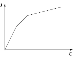
Concavity: Consider the(mn+2)-dimensional space with the mn variables xk jand, additionally, εand u as coordinates. Let F be the feasible region of our linear program in this space, that is, the set of(mn+2)-vectors that fulfill constraints (2),(3),(4). Clearly, F is convex. Hence the projection F|ε,u of F to the εvs. u plane is convex, too. (F|ε,u is the set of all pairs(ε,u) for which there exist values of the xk jso that the constraints are satisfied.) Remember that we have to maximize u for a givenε. Geometrically this means to take the point at the upper boundary of F|ε,uat abscissa ε. Since F|ε,u is convex, the upper boundary is the graph of a (piecewise linear) concave function. (Figure 1.)
6
u
ε
Figure 1. u is monotone and concave inε. The graph limits the the feasible region from above.
One might expect that also every single variable xk jin the strategy matrix X is monotone in the error boundε, but this is not true in general. A small example demonstrates the reason. Recall the notations pk j for the probability to observe Ok given Hj, the weighted row sums xk :=∑ni=1wixki, and the utility-to-size ratios rk j:=wj∑ni=1pkiqi/pk jfrom the fractional knapsack problems. Example 1 Suppose that all hypotheses have unit weights wj=1. Consider the following matrix P of conditional probabilities pk j:
P=
0.1 0.5 0.8 0.9 0.5 0.2
.
satisfies the criterion in Theorem 6. Hence
X∗=
0.73+x 0 0 0.03−x 0.2 0.5
with 0≤x≤0.03 (arbitrary) is optimal, and(1,0,0)is a worst prior. This in turn implies that every optimal X must be a knapsack solution against(1,0,0). In particular, x22=0.2 is enforced.
Now let ε=0.2 instead. Then, every knapsack solution against(1,0,0) has x1<x2, so that prior(0,0,1)would be worse. But, similarly, every knapsack solution against(0,0,1)has x1>x2, so that prior(1,0,0)would be worse. It follows that x1=x2holds in every optimal X , and that an optimal q∗ differs from these two priors. But each prior except the mentioned two gives r11>r21 and r23>r13, which determines column 1 and 3 of X∗ uniquely. Together with x1=x2 this finally yields (matrix entries rounded to three decimals):
X∗=
1 0.256 0 0.111 0.144 1
.
Note that x22 is smaller than before! The explanation is that x11 reached 1, thus only x21 could increase, and x22decreased in favour of x12, in order to keep x1and x2balanced.
Next we consider arbitrary individual error boundsεj again. As announced, we show that our linear programs from Theorem 2 have optimal solutions where only a minority of the mn variables xk j is fractional, that is, properly between 0 and 1. It means that these selection strategies are to a large extent deterministic, which makes them much easier to handle in practice.
Theorem 8 Any optimal solution being a vertex of the feasible region has at most 2n fractional variables.
Proof Some optimal solution X of a linear program is always a vertex of the feasible region. Con-straints (4) describe the hypercube in mn-dimensional space where all vertices have coordinates 0 or 1. Furthermore, the number of binding constraints in a vertex X is at least the dimension mn, but only one of any two constraints xk j≥0, xk j≤1 can be binding. Thus, in a vertex X with more than 2n fractional coordinates, more than 2n other constraints must be binding. Since we have only 2n constraints (2),(3), the assertion follows.
We can also say something about the positions of fractional entries in optimal strategy matrices X and get a better bound in case that m≤n. Let B(X) be the bipartite graph with vertices rk for all rows k, and vertices cj for all columns j, where an edge between rk and cj exists iff xk j is a fractional value.
Theorem 9 There exists an optimal solution X with cycle-free B(X), and thus at most m+n−1 fractional entries.
rows and columns in X is arbitrary, hence we may rename them such that, without loss of generality, indices in C are 1,2, . . . ,l as defined above.
Let d be some real number that we fix later. We change the matrix entries corresponding to the edges in C by the following procedure. First, define d11=d and replace x11with x11−d11. Define d21 = pp1121d11 and replace x21 with x21+d21. Obviously, the error bound constraint (2) remains valid for column j=1. Next, define d22=ww12d21and replace x22with x22−d22. The effect is that xk :=∑ni=1wixkiremains unchanged for row k=2. We walk the cycle C and continue in this way. The general step is: Define dii=wi−1
wi di,i−1and replace xiiwith xii−dii, then define di+1,i= pii pi+1,1dii and replace xi+1,iwith xi+1,i+di+1,1. Following this scheme we finally we update x1l, according to
l+1 mod l=1.
Note that all these changes neither affect the left-hand sides of constraints (2) nor the weighted row sums xk defined above, with x1as the only exception. If x1 has not decreased, constraints (3) remain satisfied, too. If x1has decreased, we use−d instead of d, so that x1 now increases. Since all xk jon edges of C are fractional, constraints (4) also remain valid for small enough|d|. Hence we get a new feasible solution for any d which has the suitable sign and small enough absolute value. Finally we adjust our d so that some entry in C becomes exactly 0 or 1.
Hence we can destroy some cycle C of fractional entries. Since the optimal value u is monotone in the xk, the new solution X is no worse. Applying the same procedure repeatedly we destroy all such cycles. Since every step also properly decreases the number of fractional entries, the process terminates with an X as desired. Since a cycle-free graph has fewer edges than vertices, the bound m+n−1 follows.
We remark that this proof gives also a polynomial algorithm that computes a cycle-free optimal solution.
The 3×2 instances from Example 1 admit optimal solutions with n=3 fractional entries. An obvious question is whether our combinatorial bounds are already tight. More precisely: Given numbers m,n, let f(m,n)denote the largest number such that there exists an m×n instance P of HYPOTHESIS SELECTION WITH ERRORBOUNDS where every optimal solution X needs at least f(m,n)fractional variables. We have shown f(m,n)≤min{m,n}+n, and it is trivial to give general examples where the number of fractional variables must be n, so that f(m,n)≥n. On the other hand, note that the “fractional knapsack” property of optimal solutions does not imply f(m,n)≤n: Knapsack solutions are not always unique and may allow several fractional variables in a column j (namely if several rk jare equal), and since a knapsack solution against a dual optimal q∗is not necessarily already optimal, we may have to take a solution with more fractional variables. We must leave the exact f(m,n)as an open problem.
5. Is There a Faster Algorithm?
In this more informal section we briefly discuss another open problem: to devise a purely combina-torial algorithm for our class of linear programs that is faster than a generic linear program solver. We point out two ways, but also the reasons why these attempts have not been successful so far.
due to the following discussion. Let us call two matrix entries in the same row or column a monotone pair if the values of these entries in X and P stand in the same relation (larger or smaller). For an input P and a strategy X , define a directed graph C(X) whose vertices are the columns, with a directed arc from i to j if pki>pk jand xki>xk jholds for some k. The directed graph R(X)whose vertices are rows is defined similarly. By an argument similar to the proof of Theorem 9 we can show the existence of an optimal solution X where B(X)is cycle-free and also C(X)and R(X)are free of directed cycles. Hence there is some topological order of the rows and columns such that all monotone pairs in rows and columns decrease in the same direction, for example, to the right and downwards, respectively. However this does not limit the number of monotone pairs. Moreover, the topological orders are not obvious from P, and even if we knew them, we could not compute the optimal X from them in a simple way. In summary, the observation above did not lead us to an efficient algorithm.
(2) Another idea is a reduction to flow problems in bipartite lossy networks. For that problem which has many other applications in transportation and finance (for example, currency exchange), purely combinatorial polynomial-time algorithms have been given by Tardos and Wayne (1998); Wayne (2002). However, the idea works only for a variant of HYPOTHESIS SELECTION WITH
ERRORBOUNDSwith “observation-wise” exclusiveness demands instead of a global exclusiveness objective: Recall again the weighted row sums xk:=∑ni=1wixki. For given parametersεj and yk for all j and k, respectively, we may raise the following existence problem: Is there a solution X with error probabilities at most εj for all Hj, and xk ≥yk for all Ok? This problem is easily seen to be a flow problem in a bipartite lossy network with arc capacities 1 and gain factors 1/pk j; see Tardos and Wayne (1998); Wayne (2002) for the definitions. In contrast, a reduction from HYPOTHESIS SELECTION WITHERRORBOUNDS does not seem to exist, for the intuitive reason that flow variables cannot be “copied” in order to “participate” in several linear combinations of the xk. Still, algorithmic techniques similar to those used for flows in lossy networks might be applicable. We have to leave this subject for future research.
6. Combining Data
Suppose that we have several matrices P(1),P(2), . . .of conditional probabilities for the same set of hypotheses but for different types of observations, such as different groups of symptomes in diagnosis, or chemical shifts of several nuclei in protein torsion angle prediction. We do not assume that the joint distribution of vectors of observations is known: Since the number of vectors is the product of m(1),m(2), . . ., there may be not enough cases in the database that would allow meaningful probability estimates for all these vectors. Still, combining these data sets can further narrow down the selected hypotheses (if the observations “complement each other” well), and at the same time preserve guaranteed error bounds. For ease of presentation we describe the method for two matrices, but it can be readily extended to any number.
Proof In fact, the combined strategy is designed so that we discard any Hjif at least one of the pre-dictors X or X′does. The decision to discard a hypothesis is taken independently in both instances. Hence, if Ok,O′l are observed, we keep Hj with probability
(1−xk j)(1−x′l j) =1−(xk j+x′l j−xk jx′l j).
On the other hand, since the probability of a union of events is at most the sum of probabilities of the single events, we discard target Hj with at most the probabilityεj+ε′j.
Proposition 10 gives only a guarantee on the error probabilities. However, concavity of exclu-siveness (see Proposition 7) suggests that combining two predictors with half error bound in general improves the exclusiveness. For concrete instances and a desired total error probability we may try various partitions into summands, with some resonable step length, and take the combination that works best. We also remark that, since by Theorem 8 and 9 most strategy variables xk j,x′l j are 0 or 1, the calculations are fast.
If several P(i)are available (for example, in our protein structure application, the chemical shifts of 6 nuclei, and also from neighbored residues), then exhaustive search is expensive, but we may choose to combine only the most informative data, that is, only those P(i)with largest exclusiveness.
Finally, a deliberately very simple, symmetric toy example with two hypotheses of equal weight illustrates the principle of combining predictions.
Example 2
P=
1 0.5 0 0.5
P′=
0.5 1 0.5 0
We choose ε=0.2 for both hypotheses in both instances. Then the optimal solutions for the separate instances are, rather obviously:
X=
0.2 0.4
1 0
X′=
0.4 0.2
0 1
.
In the first instance, the exclusiveness is only 0.6 if H1is the target (since always O1is observed), and for H2 we get exclusiveness 0.8 (average of both rows), the second instance is symmetric. If we use the information from both instances, we can improve the exclusiveness for the sameε=0.2. First we optimize both instances separately, but now with half error bound 0.1:
X=
0.1 0.2
1 0
X′=
0.2 0.1
0 1
.
For the four combinations (k,l) = (1,1),(1,2),(2,1),(2,2)we compute new exclusion proba-bilities as specified above:
0.28 0.28 0.1 1
1 0.1
1 1
.
7. Application Note: Protein Torsion Angle Prediction
We studied properties of a class of linear programs for hypotheses selection in probabilistic infer-ence which is hopefully of fundamental interest. We were led to the problem class by a concrete challenge: a project where we are comparing different methods for predicting protein torsion angles from NMR chemical shifts, see Section 1. Characteristic features of our scatterplot data are large empty regions with almost no data points, in them clouds of data points with a variety of shapes and different densities. Optimization assists in the creation of a predictor:
Any prediction heuristic has to take a measured chemical shift value and output predicted torsion angle values. In a statistical approach it is sensible to precompute the predictions, based on the sampled data. The actual application is then a simple table look-up, done by an auxiliary program. The main relevant question for spectroscopists is the achievable confidence when predicting torsion angle intervals of a prescribed length (error probability vs. exclusiveness, in our terminology). Then they can make their specific decisions using this tradeoff. Besides the actual predictions, the optimization results also quantify how informative the chemical shifts of different nuclei (or their combinations) are for this purpose.
Basic heuristics working purely “row-wise” (MAP, ML, or similar) do not pay attention to error probabilities for specific hypothesis intervals and easily discard certain torsion angles completely, despite a considerable frequency of occurrence. Hence such heuristics generate systematically mis-leading predictions when these neglected ranges of torsion angles appear. Even worse, they can appear more frequently in a protein under consideration than in the database: Recall that the scatter-plots are sampled from a large collection of various proteins so that we know only average torsion angle frequencies. A more even distribution of errors to different torsion angles gives more robust-ness against varying torsion angle frequencies. We can also expect that the global structure recon-struction process itself works smoother if the local restraints have balanced errors: Most wrong sequences of torsion angles, that is, sequences with errors injected, are already geometrically im-possible, which gives us a chance to correct such occasional errors.1 Since the precise effects are hard to know beforehand, free parametersεj seem to be a valuable feature.
A simple MAP heuristics, for example, would take the measured chemical shift value and select the torsion angle ranges (columns) with highest point densities in the row containing the measured value. Other preferences may be taken into account, for instance, one interval is easier to handle as a restraint than a union of several intervals. In either case, a selection yields a matrix X and a vector of error probabilitiesεj which are typically low (high) in densely (sparsely) populated columns. Now we can adjust error probabilities for individual torsion angle intervals in any desired direction and re-optimize.
As an illustration we discuss an arbitrary example (point count matrix) from the real data: As-partic Acid, nucleus Cα, and torsion angleφ, partitioned into homogeneous regions using the method from Christin (2006):
1 0 7 12 4 1 1 0
0 0 0 19 18 1 2 0
5 4 22 212 116 16 4 0
2 3 21 90 32 3 5 0
10 6 38 93 28 7 39 3 98 86 304 193 39 11 63 5 34 43 86 27 4 0 7 3 22 60 67 18 1 1 2 2
3 12 19 6 4 0 2 0
40 30 30 20 15 80 45 100
.
The bottom line gives the torsion angle interval lengths in degrees, that is, our weights. The frequencies of hypotheses in the database are (in percent, rounded):
8.5 10.5 27.5 33.0 12.0 2.0 6.0 0.5
.
Suppose we want to predict torsion angle intervals of about 60 degrees and start with a naive MAP heuristic that takes the intervals of exactly 60 degrees with maximum density in each row. It leads to the following matrix X (entries indicate the discarded fractions of intervals, values are rounded):
1 1 0.17 0 0 1 1 1 1 1 1 0 0 0.69 1 1 1 1 0.17 0 0 1 1 1 1 1 0.17 0 0 1 1 1 1 1 0.17 0 0 1 1 1 1 0.67 0 0 1 1 1 1
1 0 0 1 1 1 1 1
1 0 0 1 1 1 1 1
1 0 0 1 1 1 1 1
100.0 33.0 2.5 7.5 19.5 99.0 100.0 100.0
.
The bottom line indicates the error boundsεj in percent (rounded). For the prior probabilities from the database, the overall error probability would be about 26%. Optimization with the sameεj yields only marginal changes:
1 1 0 0 0 1 1 1
1 1 1 0 0 0.69 1 1 1 1 0.18 0 0 1 1 1 1 1 0.16 0 0 1 1 1 1 1 0.17 0 0 1 1 1 1 0.67 0 0 1 1 1 1
1 0 0 1 1 1 1 1
1 0 0 1 1 1 1 1
1 0 0.06 1 1 1 1 1
Columns 6 and 8 are completely discarded, which is reasonable because only 2.5% of cases are to be expected in the corresponding large intervals. The separate cluster in column 7 which appeared with 6% is always discarded, too. We may accept this error when we prefer a single predicted interval to a union of two (see the remark above). The most relevant part is the dense region in columns 1 to 5. Observe that also column 1 is completely discarded, even though it contains a considerable cluster of points. This makes up for 8.5 of the 26% total error. Let us reduce ε1 and see how this affects the predictions. For instance, after changing ε1 to 0.4, optimization (followed by raising some sporadic xk j<1 to 1 when pk jis small) yields this X :
1 1 0 0 0 1 1 1
1 1 1 0 0 0.69 1 1
1 1 0 0 0 1 1 1
0.76 0 0 0 0 1 1 1
1 1 0 0 0 1 1 1
0.26 0.7 0 0.03 1 1 1 1 0.16 0 0.16 1 1 1 1 1
1 0 0 1 1 1 1 1
1 0 0 0 1 1 1 1
.
We remark that the optimal dual solution moved from q3=1 to q1=1. The (expected) length of predicted intervals increased to 84 degrees. On the other hand, the global error went down to 21%, and we can afford to raise the very small initialε3. For instance, withε3=0.2 we are back to the initial total error of 26%, now with an expected hypothesis length of 77 degrees and the following X :
1 1 0 0 0 1 1 1
1 1 1 0 0 0.69 1 1
1 1 0 0 0 1 1 1
1 0.06 0 0 0 1 1 1
1 1 0 0 0 1 1 1
0.46 0.7 0 0 1 1 1 1
0 0 1 1 1 1 1 1
0.16 0 0.4 1 1 1 1 1
1 0 0 1 1 1 1 1
.
Interestingly, this step pressed the predictions in rows 7,8 more to the lower left corner, while x61became higher again. The apparent reason is that, in row 6, the element in column 1 has strong competitors in columns 3 and 4. Hence it is not predicted definitely, even though p61>p71,p81. The result in row 6 suggests to choose either columns 1-2 or 3-4. In order to avoid predicting intervals of excessive lengths in some rows, we may cut the longest intervals down, for example, at the end with the smallest increase of error. In our example, the longest predicted interval, with 93 degrees, appears in row 4. Changing x42to 1 increasesε2marginally to 0.345 but shortens this interval to 65 degrees. In row 8 we may cut at column 3, etc.
plausible heuristics: εj proportional to the weight-by-frequency ratio, equalεj, and combinations of them. However, since no simple automatic rule seems to be satisfactory for all diverse shapes of scatterplots (apparently bad examples exist for each), some minor intervention as shown above is required.
Acknowledgments
The first author has been supported by the Knut and Alice Wallenberg Foundation, Carl Tryggers Foundation, and Assar Gabrielsson Foundation. The second author has been partially supported by the Swedish Research Council (Vetenskapsr˚adet), grant no. 621-2002-4574.
We thank the anonymous referees for their helpful suggestions.
References
R. D. Beger and P. H. Bolton. Protein φandψ dihedral restraints determined from multidimen-sional hypersurface correlations of backbone chemical shifts and their use in the determination of protein tertiary structures. Journal of Biomolecular NMR, 10:129–142, 1997.
K. P. Bennett. Decision tree construction via linear programming. In Proceedings of the 4th Midwest AI and Cognitive Science Sociecty Conference, pages 97–101, 1992.
K. P. Bennett and O. L. Mangasarian. Neural network training via linear programming. In Advances in Optimization and Parallel Computing, pages 56–67. North-Holland, 1992a.
K. P. Bennett and O. L. Mangasarian. Robust linear programming discrimination of two linearly inseparable sets. Optimization Methods and Software, 1:23–34, 1992b.
K. P. Bennett and O. L. Mangasarian. Multicategory separation via linear programming. Optimiza-tion Methods and Software, 3:27–39, 1993.
P. S. Bradley. Mathematical Programming Approaches to Machine Learning and Data Mining. PhD thesis, University of Wisconsin, 1998.
C. Christin. Scatterplot partitioning algorithm for LETA-NMR. Master’s thesis, International Mas-ter’s Programme in Bioinformatics, Chalmers University, G¨oteborg (Sweden), 2006.
G. Cornilescu, F. Delaglio, and A. Bax. Protein backbone angle restraints from searching a database for chemical shift and sequence homology. Journal of Biomolecular NMR, 13:289–302, 1999.
P. Damaschke. Scheduling search procedures. Journal of Scheduling, 7:349–364, 2004.
F. Glover. Improved linear programming models for discriminant analysis. Decision Sciences, 21: 771–785, 1990.
S. Martello and P. Toth. Knapsack Problems: Algorithms and Computer Implementations. Wiley, 1990.
E. Tardos and K. D. Wayne. Simple generalized maximum flow algorithms. In Proceedings of the 6th Integer Programming and Combinatorial Optimization Conference, Lecture Notes in Com-puter Science, volume 1412, pages 310–324, 1998.
Y. Wang and O. Jardetzky. Probability-based protein secondary structure identification using com-bined NMR chemical-shift data. Protein Science, 11:852–861, 2002.
K. D. Wayne. A polynomial combinatorial algorithm for generalized minimum cost flow. Mathe-matical Operations Research, 27:445–459, 2002.