Large Scale Transductive SVMs

(1)

Large Scale Transductive SVMs

Ronan Collobert [email protected]

NEC Laboratories America 4 Independence Way Princeton, NJ 08540, USA

Fabian Sinz [email protected]

NEC Laboratories America 4 Independence Way

Princeton, NJ 08540, USA, and

Max Planck Institute for Biological Cybernetics Spemannstrasse 38

72076 Tuebingen, Germany

Jason Weston [email protected]

L´eon Bottou [email protected]

NEC Laboratories America 4 Independence Way Princeton, NJ 08540, USA

Editor: Thorsten Joachims

Abstract

We show how the concave-convex procedure can be applied to transductive SVMs, which tradition-ally require solving a combinatorial search problem. This provides for the first time a highly scal-able algorithm in the nonlinear case. Detailed experiments verify the utility of our approach. Soft-ware is available athttp://www.kyb.tuebingen.mpg.de/bs/people/fabee/transduction. html.

Keywords: transduction, transductive SVMs, semi-supervised learning, CCCP

1. Introduction

Transductive support vector machines (TSVMs) (Vapnik, 1995) are a method of improving the generalization accuracy of SVMs (Boser et al., 1992) by using unlabeled data. TSVMs, like SVMs, learn a large margin hyperplane classifier using labeled training data, but simultaneously force this hyperplane to be far away from the unlabeled data.

(2)

it seems clear that algorithms such as TSVMs can give considerable improvement in generalization over SVMs, if the number of labeled points is small and the number of unlabeled points is large.

Unfortunately, TSVM algorithms (like other semi-supervised approaches) are often unable to deal with a large number of unlabeled examples. The first implementation of TSVM appeared in (Bennett and Demiriz, 1998), using an integer programming method, intractable for large prob-lems. Joachims (1999b) then proposed a combinatorial approach, known as SVMLight-TSVM, that is practical for a few thousand examples. Fung and Mangasarian (2001) introduced a sequential op-timization procedure that could potentially scale well, although their largest experiment used only 1000 examples. However, their method was for the linear case only, and used a special kind of SVM with a 1-norm regularizer, to retain linearity. Finally, Chapelle and Zien (2005) proposed a primal method, which turned out to show improved generalization performance over the previous approaches, but still scales as(L+U)3_{, where L and U are the numbers of labeled and unlabeled} examples. This method also stores the entire(L+U)×(L+U)kernel matrix in memory. Other methods (Bie and Cristianini, 2004; Xu et al., 2005) transform the non-convex transductive problem into a convex semi-definite programming problem that scales as(L+U)4_{or worse.}

In this article we introduce a large scale training method for TSVMs using the concave-convex procedure (CCCP) (Yuille and Rangarajan, 2002; Le Thi, 1994), expanding on the conference pro-ceedings paper (Collobert et al., 2006). CCCP iteratively optimizes non-convex cost functions that can be expressed as the sum of a convex function and a concave function. The optimization is car-ried out iteratively by solving a sequence of convex problems obtained by linearly approximating the concave function in the vicinity of the solution of the previous convex problem. This method is guaranteed to find a local minimum and has no difficult parameters to tune. This provides what we believe is the best known method for implementing transductive SVMs with an empirical scaling of

(L+U)2_{, which involves training a sequence of typically 1-10 conventional convex SVM} optimiza-tion problems. As each of these problems is trained in the dual we retain the SVM’s linear scaling with problem dimensionality, in contrast to the techniques of Fung and Mangasarian (2001).

2. The Concave-Convex Procedure for TSVMs

Notation We consider a set of L training pairs

L

={(x1,y1), . . . ,(xL,yL)},x∈Rn, y∈ {1,−1}

and an (unlabeled) set of U test vectors

U

={xL+1, . . . ,xL+U}. SVMs have a decision function fθ(.)

of the form

fθ(x) =w·Φ(x) +b,

whereθ= (w,b)are the parameters of the model, andΦ(·)is the chosen feature map, often imple-mented implicitly using the kernel trick (Vapnik, 1995).

TSVM Formulation The original TSVM optimization problem is the following (Vapnik, 1995; Joachims, 1999b; Bennett and Demiriz, 1998). Given a training set

L

and a test set

U

, find among the possible binary vectors

{

Y

= (yL+1, . . . ,yL+U)}

the one such that an SVM trained on

L

∪(

U

×

Y

)yields the largest margin.

(3)

−30 −2 −1 0 1 2 3 0.2

0.4 0.6 0.8 1

z −3 −2 −1 0 1 2 3

0 0.2 0.4 0.6 0.8 1

z −3 −2 −1 0 1 2 3

0 0.1 0.2 0.3 0.4 0.5 0.6

z

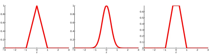
Figure 1: Three loss functions for unlabeled examples, from left to right (i) the Symmetric Hinge H1(|t|) =max(0,1−|t|), (ii) Symmetric Sigmoid S(t) =exp(−3t2); and (iii) Symmetric Ramp loss, Rs(|t|) =min(1+s,max(0,1− |t|)). The last loss function has a plateau of

width 2|s|where s∈(−1,0]is a tunable parameter, in this case s=−0.3.

as possible from the margin. This can be written as minimizing

1 2kwk

2₊_C

∑

L

i=1

ξi+C∗ L+U

∑

i=L+1

ξi

subject to

yifθ(xi)≥1−ξi, i=1, . . . ,L

|fθ(xi)| ≥1−ξi, i=L+1, . . . ,L+U

This minimization problem is equivalent to minimizing

J(θ) =1

2kwk

2₊_C

∑

L

i=1

H1(yifθ(xi)) +C∗ L+U

∑

i=L+1

H1(|fθ(xi)|), (1)

where the function H1(·) =max(0,1− ·) is the classical Hinge Loss (Figure 2, center). The loss function H1(| · |) for the unlabeled examples can be seen in Figure 1, left. For C∗=0 in (1) we obtain the standard SVM optimization problem. For C∗ >0 we penalize unlabeled data that is inside the margin. This is equivalent to using the hinge loss on the unlabeled data as well, but where we assume the label for the unlabeled example is yi=sign(fθ(xi)).

Losses for transduction TSVMs implementing formulation (1) were first introduced in SVM-Light (Joachims, 1999b). As shown above, it assigns a Hinge Loss H1(·)on the labeled examples (Figure 2, center) and a “Symmetric Hinge Loss” H1(| · |)on the unlabeled examples (Figure 1, left). More recently, Chapelle and Zien (2005) proposed to handle unlabeled examples with a smooth ver-sion of this loss (Figure 1, center). While we also use the Hinge Loss for labeled examples, we use for unlabeled examples a slightly more general form of the Symmetric Hinge Loss, that we allow to be “non-peaky” (Figure 1, right). Given an unlabeled examplexand using the notation z= fθ(x),

this loss can be written as

z7→Rs(z) +Rs(−z) +const.1, (2)

where−1<s≤0 is a hyper-parameter to be chosen and Rs=min(1−s,max(0,1−t))is what we

call the “Ramp Loss”, a “clipped” version of the Hinge Loss (Figure 2, left).

(4)

Losses similar to the Ramp Loss have been already used for different purposes, like in the Doom II algorithm (Mason et al., 2000) or in the context of “Ψ-learning” (Shen et al., 2003). The s parameter controls where we clip the Ramp Loss, and as a consequence it also controls the wideness of the flat part of the loss (2) we use for transduction: when s=0, this reverts to the Symmetric Hinge H1(| · |). When s6=0, we obtain a non-peaked loss function (Figure 1, right) which can be viewed as a simplification of Chapelle’s loss function. We call this loss function (2) the “Symmetric Ramp Loss”.

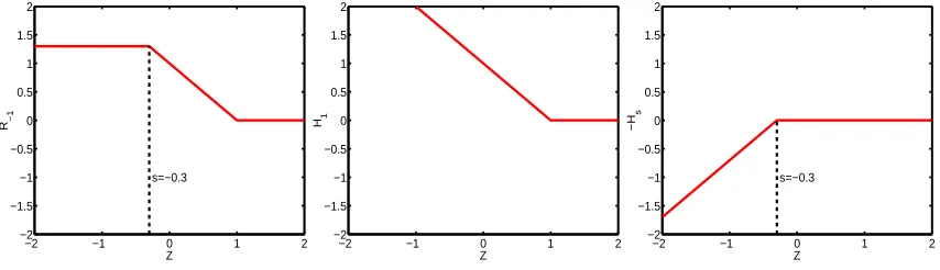
−2 −1 0 1 2

−2 −1.5 −1 −0.5 0 0.5 1 1.5 2 s=−0.3 Z R−1

−2 −1 0 1 2

−2 −1.5 −1 −0.5 0 0.5 1 1.5 2 Z H1

−2 −1 0 1 2

−2 −1.5 −1 −0.5 0 0.5 1 1.5 2 s=−0.3 Z −H s

Figure 2: The Ramp Loss function Rs(t) =min(1−s,max(0,1−t)) =H1(t)−Hs(t)(left) can be

decomposed into the sum of the convex Hinge Loss (center) and a concave loss (right), where Hs(t) =max(0,s−t). The parameter s controls the cutoff point of the usual Hinge

loss.

Training a TSVM using the loss function (2) is equivalent to training an SVM using the Hinge loss H1(·)for labeled examples, and using the Ramp loss Rs(·)for unlabeled examples, where each

unlabeled example appears as two examples labeled with both possible classes. More formally, after introducing

yi = 1 i∈[L+1. . .L+U]

yi = −1 i∈[L+U+1. . .L+2U]

xi = xi−U i∈[L+U+1. . .L+2U],

we can rewrite (1) as

Js(θ) =1

2kwk

2₊_C

∑

L

i=1

H1(yifθ(xi)) +C∗ L+2U

∑

i=L+1

Rs(yifθ(xi)). (3)

This is the minimization problem we now consider in the rest of the paper.

Balancing constraint One problem with TSVM as stated above is that in high dimensions with few training examples, it is possible to classify all the unlabeled examples as belonging to only one of the classes with a very large margin, which leads to poor performance. To cure this problem, one further constrains the solution by introducing a balancing constraint that ensures the unlabeled data are assigned to both classes. Joachims (1999b) directly enforces that the fraction of positive and negatives assigned to the unlabeled data should be the same fraction as found in the labeled data. Chapelle and Zien (2005) use a similar but slightly relaxed constraint, which we also use in this work:

1 U

L+U

∑

i=L+1

fθ(xi) =

1 L

L

∑

i=1

(5)

Concave-Convex Procedure (CCCP) Unfortunately, the TSVM optimization problem as given above is not convex, and minimizing a non-convex cost function is often considered difficult. Gra-dient descent techniques, such as conjugate graGra-dient descent or stochastic graGra-dient descent, often involve delicate hyper-parameters (LeCun et al., 1998). In contrast, convex optimization seems much more straight-forward. For instance, the SMO algorithm (Platt, 1999) locates the SVM solu-tion efficiently and reliably.

We propose to solve this non-convex problem using the “Concave-Convex Procedure” (CCCP) (Yuille and Rangarajan, 2002). The CCCP procedure is closely related to the “Difference of Con-vex” (DC) methods that have been developed by the optimization community during the last two decades (Le Thi, 1994). Such techniques have already been applied for dealing with missing values in SVMs (Smola et al., 2005), for improving boosting algorithms (Krause and Singer, 2004), and in the “Ψ-learning” framework (Shen et al., 2003).

Assume that a cost function J(θ) can be rewritten as the sum of a convex part Jvex(θ) and

a concave part Jcav(θ). Each iteration of the CCCP procedure (Algorithm 1) approximates the

concave part by its tangent and minimizes the resulting convex function.

Algorithm 1 : The concave-convex procedure (CCCP)

Initializeθ0_{with a best guess.}

repeat

θt+1=arg min

θ

Jvex(θ) +Jcav′ (θt)·θ

(5)

until convergence ofθt

One can easily see that the cost J(θt₎_{decreases after each iteration by summing two inequalities}

resulting from (5) and from the concavity of Jcav(θ).

Jvex(θt+1) +Jcav′ (θt)·θt+1 ≤ Jvex(θt) +Jcav′ (θt)·θt (6)

Jcav(θt+1) ≤ Jcav(θt) +Jcav′ (θt)· θt+1−θt

(7)

The convergence of CCCP has been shown by Yuille and Rangarajan (2002) by refining this argu-ment. The authors also showed that the CCCP procedure remains valid ifθ is required to satisfy some linear constraints. Note that no additional hyper-parameters are needed by CCCP. Further-more, each update (5) is a convex minimization problem and can be solved using classical and efficient convex algorithms.

CCCP for TSVMs Interestingly, the Ramp Loss can be rewritten as the difference between two Hinge losses (see Figure 2):

Rs(z) =H1(z)−Hs(z). (8)

(6)

J_cavs (θ)part as follows:

Js(θ) =1

2kwk

2₊_C

∑

L

i=1

∑

i=L+1

Rs(yifθ(xi))

= 1

2kwk

2₊_C

∑

L

i=1

H1(yi fθ(xi)) +C∗ L+2U

∑

i=L+1

H1(yifθ(xi))

| {z }

J_vexs (θ)

−C∗

L+2U

∑

i=L+1

Hs(yifθ(xi))

| {z }

J_cavs (θ)

.

(9)

This decomposition allows us to apply the CCCP procedure as stated in Algorithm 1. The convex optimization problem (5) that constitutes the core of the CCCP algorithm is easily reformulated into dual variablesαusing the standard SVM technique.

After some algebra, we show in Appendix A that enforcing the balancing constraint (4) can be achieved by introducing an extra Lagrangian variableα0and an examplex0implicitely defined by

Φ(x0) = 1 U

L+U

∑

i=L+1

Φ(xi),

with label y0=1. Thus, if we note K the kernel matrix such that

Ki j=Φ(xi)·Φ(xj),

the column corresponding to the examplex0is computed as follow:

Ki0=K0i= 1 U

L+U

∑

j=L+1

Φ(xj)·Φ(xi) ∀i. (10)

The computation of this special column can be achieved very efficiently by computing it only once, or by approximating the sum (10) using an appropriate sampling method.

Given the decomposition of the cost (9) and the trick of the special extra example (10) to enforce the balancing constraint, we can easily apply Algorithm 1 to TSVMs. To simplifiy the first order approximation of the concave part in the CCCP procedure (5), we denote

βi = yi

∂J_cavs (θ) ∂fθ(xi)

=

C∗ if yi fθ(xi)<s

0 otherwise , (11)

for unlabeled examples (that is i≥L+1).2 The concave part J_cavs does not depend on labeled examples (i≤L) so we obviously haveβi=0 for all i≤L. This yields Algorithm 2, after some

standard derivations detailed in Appendix A.

Convergence of Algorithm 2 in finite time t∗ is guaranteed because variable β can only take a finite number of distinct values, because J(θt₎ _{is decreasing, and because inequality (7) is strict}

unlessβremains unchanged.

(7)

Algorithm 2 : CCCP for TSVMs

Initializeθ0= (w0,b0)with a standard SVM solution on the labeled points. Computeβ0_i =

C∗ if yi fθ0(x_i)<s and i≥L+1

0 otherwise

Setζi=yifor 1≤i≤L+2U andζ0=_L1∑Li=1yi

repeat

•Solve the following convex problem ( with Ki j=Φ(xi)·Φ(xj) )

max

α

α·ζ−1

2α

T_{K α}

subject to  



α·1=0

0≤yiαi≤C ∀1≤i≤L

−βi≤yiαi≤C∗−βi ∀i≥L+1

•Compute bt+1using f_θt+1(x_i) = L+2U

∑

j=0

αt+1

j Ki j +bt+1and

∀i≤L : 0<yiαi<C =⇒ yifθt+1(x_i) =1 ∀i>L : −βi<yiαi<C∗−βi =⇒ yifθt+1(x_i) =1

• Computeβt_i+1=

C∗ if yifθt+1(x_i)<s and i≥L+1

0 otherwise

until βt+1₌_βt

Complexity The main point we want to emphasize in this paper is the advantage in terms of training time of our method compared to existing approaches. Training a CCCP-TSVM amounts to solving a series of SVM optimization problems with L+2U variables. Although SVM training has a worst case complexity of

O

((L+2U)3₎_{it typically scales quadratically (see Joachims, 1999a;} Platt, 1999), and we find this is the case for our TSVM subproblems as well. Assuming a constant number of iteration steps, the whole optimization of TSVMs with CCCP should scale quadratically in most practical cases (see Figure 3, Figure 8 and Figure 9). From our experience, around five iteration steps are usually sufficient to reach the minimum, as shown in the experimental section of this paper, Figure 4.

3. Previous Work

SVMLight-TSVM Like our work, the heuristic optimization algorithm implemented in SVM-Light (Joachims, 1999b) solves successive SVM optimization problems, but on L+U instead of L+2U data points. It improves the objective function by iteratively switching the labels of two unlabeled pointsxi andxj withξi+ξj>2. It uses two nested loops to optimize a TSVM which

(8)

SVMLight uses annealing heuristics for the selection of C∗. It begins with a small value of C∗ (C∗=1e−5), and multiplies C∗by 1.5 on each iteration until it reaches C. The numbers 1e−5 and 1.5 are hard coded into the implementation. On each iteration the tolerance on the gradients is also changed so as to give more approximate (but faster) solutions on earlier iterations. Again, several heuristics parameters are hard coded into the implementation.

∇TSVM The∇TSVM of Chapelle and Zien (2005) is optimized by performing gradient descent in the primal space: minimize

1 2kwk

2₊_C

∑

L

i=1

H2(yifθ(xi)) +C∗ L+U

∑

i=L+1

H∗(yifθ(xi)),

where H2(t) =max(0,1−t)2 _{and H}∗₍_t_{) =}_exp₍₋_3t2₎ _{(cf. Figure 1, center). This optimization} problem can be considered a smoothed version of (1).∇TSVM also has similar heuristics for C∗as SVMLight-TSVM. It begins with a small value of C∗(C∗=bC), and iteratively increases C∗over l iterations until it finally reaches C. The values b=0.01 and l=10 are default parameters in the code available at:http://www.kyb.tuebingen.mpg.de/bs/people/chapelle/lds.

Since the gradient descent is carried out in the primal, to learn nonlinear functions it is necessary to perform kernel PCA (Sch¨olkopf et al., 1997). The overall algorithm has a time complexity equal to the square of the number of variables times the complexity of evaluating the cost function. In this case, evaluating the objective scales linearly in the number of examples, so the overall worst case complexity of solving the optimization problem for∇TSVM is

O

((U+L)3₎_{. The KPCA calculation} alone also has a time complexity of

O

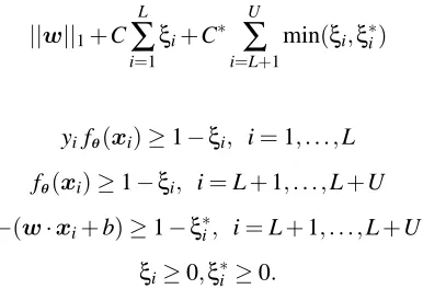
((U+L)3₎_{. This method also requires one to store the entire} kernel matrix in memory, which clearly becomes infeasible for large data sets.

CS3VM The work of Fung and Mangasarian (2001) is algorithmically the closest TSVM approach to our proposal. Following the formulation of transductive SVMs found in Bennett and Demiriz (1998), the authors consider transductive linear SVMs with a 1-norm regularizer, which allow them to decompose the corresponding loss function as a sum of a linear function and a concave function. Bennett proposed the following formulation which is similar to (1): minimize

||w||1+C

L

∑

i=1

ξi+C∗ U

∑

i=L+1

min(ξi,ξ∗i)

subject to

yifθ(xi)≥1−ξi, i=1, . . . ,L

fθ(xi)≥1−ξi, i=L+1, . . . ,L+U

−(w·xi+b)≥1−ξ∗i, i=L+1, . . . ,L+U ξi≥0,ξ∗i ≥0.

(9)

Note also that the algorithm presented in their paper did not implement a balancing constraint for the labeling of the unlabeled examples as in (4). Our transduction algorithm is nonlinear and the use of kernels, solving the optimization in the dual, allows for large scale training with high dimensionality and number of examples.

4. Small Scale Experiments

This section presents small scale experiments appropriate for comparing our algorithm with ex-isting TSVM approaches. In order to provide a direct comparison with published results, these experiments use the same setup as (Chapelle and Zien, 2005). All methods use the standard RBF kernel,Φ(x)·Φ(x′) =exp(−γ||x−x′||2₎_.

data set classes dims points labeled

g50c 2 50 500 50

Coil20 20 1024 1440 40

Text 2 7511 1946 50

Uspst 10 256 2007 50

Table 1: Small-Scale Data Sets. We used the same data sets and experimental setup in these exper-iments as found in Chapelle and Zien (2005).

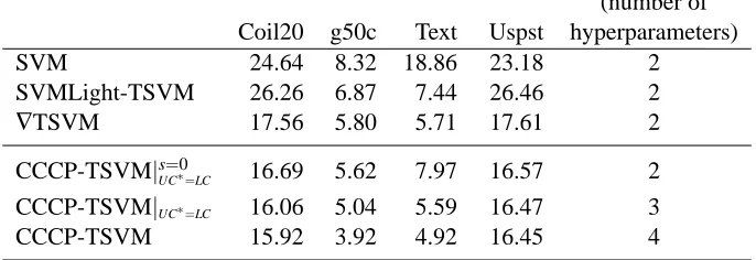
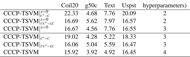
(number of Coil20 g50c Text Uspst hyperparameters)

SVM 24.64 8.32 18.86 23.18 2

SVMLight-TSVM 26.26 6.87 7.44 26.46 2

∇TSVM 17.56 5.80 5.71 17.61 2

CCCP-TSVM|s=0

UC∗=LC 16.69 5.62 7.97 16.57 2

CCCP-TSVM|UC∗=LC 16.06 5.04 5.59 16.47 3

CCCP-TSVM 15.92 3.92 4.92 16.45 4

Table 2: Results on Small-Scale Data Sets. We report the best test error over the hyperparameters of the algorithms, as in the methodology of Chapelle and Zien (2005). SVMLight-TSVM is the implementation in SVMLight. ∇TSVM is the primal gradient descent method of Chapelle and Zien (2005). CCCP-TSVM|s=0

UC∗=LCreports the results of our method using the

heuristic UC∗=LC with the Symmetric Hinge Loss, that is with s=0. We also report CCCP-TSVM|UC∗=LC where we allow the optimization of s, and CCCP-TSVM where we

allow the optimization of both C∗and s.

(10)

placed in such a way that the Bayes error is 5%. Thecoil20data is a set of gray-scale images of 20 different objects taken from different angles, in steps of 5 degrees (S.A.Nene et al., 1996). Thetext

data set consists of the classesmswindowsandmacof theNewsgroup20data set preprocessed as in Szummer and Jaakkola (2001a). Theuspstdata set is the test part of theUSPShand written digit data. All data sets are split into ten parts with each part having a small amount of labeled examples and using the remaining part as unlabeled data.

4.1 Accuracies

Consistent with (Chapelle and Zien, 2005), all hyperparameters are tuned on the test set. Chapelle and Zien (2005) argue that, in order to perform algorithm comparisons, it is sufficient to be “inter-ested in the best performance and simply select the parameter values minimizing the test error”. However we should be more cautious when comparing algorithms that have different sets of hyper-parameters. For CCCP-TSVMs we have two additional parameters, C∗and s. Therefore we report the CCCP-TSVM error rates for three different scenarios:

• CCCP-TSVM, where all four parameters are tuned on the test set.

• CCCP-TSVM|UC∗=LCwhere we choose C∗using a heuristic method. We use heuristic UC∗=

LC because it decreases C∗when the number of unlabeled data increases. Otherwise, for large enough U no attention will be paid to minimizing the training error. Further details on this choice are given in Section 4.3.

• CCCP-TSVM|s=0

UC∗=LCwhere we choose s=0 and C

∗_{using heuristic UC}∗₌_{LC. This setup has}

the same free parameters (C andγ) as the competing TSVM implementations, and therefore provides the most fair comparison.

The results are reported in Table 2. CCCP-TSVM in all three scenarios achieves approximately the same error rates as∇TSVM and appears to be superior to SVMLight-TSVM. Section 4.3 pro-vides additional results using different hyperparameter selection strategies and discusses more pre-cisely the impact of each hyperparameter.

4.2 Training Times

At this point we ask the reader to simply assume that all authors have chosen their hyperparameter selection method as well as they could. We now compare the computation times of these three algorithms.

The CCCP-TSVM algorithm was implemented in C++.3 The successive convex optimizations are performed using a state-of-the-art SMO implementation. Without further optimization, CCCP-TSVMs run orders of magnitude faster than SVMLight-CCCP-TSVMs and ∇TSVM.4 Figure 3 shows the training time on g50c and text for the three methods as we vary the number of unlabeled examples. For each method we report the training times for the hyperparameters that give optimal performance as measured on the test set on the first split of the data (we use CCCP-TSVM|s=0

UC∗=LCin

these experiments). Using all 2000 unlabeled data on Text, CCCP-TSVMs are approximately 133 times faster than SVMLight-TSVM and 50 times faster than∇TSVM.

3. Source code available athttp://www.kyb.tuebingen.mpg.de/bs/people/fabee/transduction.html. 4.∇TSVM was implemented by adapting the Matlab LDS code of Chapelle and Zien (2005) available athttp://www.

(11)

1000 200 300 400 500 10

20 30 40 50

Time (secs)

Number Of Unlabeled Examples SVMLight TSVM

∇TSVM

CCCP TSVM

0 500 1000 1500 2000 0

500 1000 1500 2000 2500 3000 3500 4000

Time (secs)

Number Of Unlabeled Examples SVMLight TSVM

∇TSVM

CCCP TSVM

Figure 3: Training times for g50c (left) and text (right) for SVMLight-TSVMs, ∇TSVMs and CCCP-TSVMs using the best parameters for each algorithm as measured on the test set in a single trial. For the Text data set, using 2000 unlabeled examples CCCP-TSVMs are

133x faster than SVMLight-TSVMs, and 50x faster than∇TSVMs.

1 2 3 40

2 4 6 8 10

Test Error

Number Of Iterations g50c

0 200 400 600 800 1000

Objective

Objective Function Test Error (%)

2 4 6 8 100

5 10 15 20 25 30

Test Error

Number Of Iterations Text

1.4 1.5 1.6 1.7 1.8 1.9x 10

6

Objective

Objective Function Test Error (%)

Figure 4: Value of the objective function and test error during the CCCP iterations of training TSVM on two data sets (single trial),g50c(left) andtext (right). CCCP-TSVM tends to converge after only a few iterations.

We expect these differences to increase as the number of unlabeled examples increases further. In particular,∇TSVM requires the storage of the entire kernel matrix in memory, and is therefore clearly infeasible for some of the large scale experiments we attempt in Section 5.

(12)

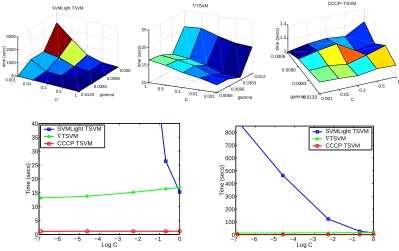
0.0006 0.0096 0.0383 0.6129 0.001 0.01 0.1 0.5 1 20 1000 2000 3000 gamma SVMLight TSVM C time (secs) 0.0006 0.0096 0.0383 0.6129 0.001 0.01 0.1 0.5 1 10 15 20 25 gamma ∇TSVM C time (secs) 0.0006 0.0096 0.0383

0.6129 0.001 0.01

0.1 0.5 1 1 1.2 1.4 C CCCP−TSVM gamma time (secs)

−70 −6 −5 −4 −3 −2 −1 0 5 10 15 20 25 30 35 40 Log C Time (secs) SVMLight TSVM ∇TSVM CCCP TSVM

−70 −6 −5 −4 −3 −2 −1 0 100 200 300 400 500 600 700 800 Log C Time (secs) SVMLight TSVM ∇TSVM CCCP TSVM

Figure 5: Computation times for different choices of hyperparameters on data setg50c(first split only) for the three TSVM implementations tested (top three figures). The bottom two figures show the computation time for all three algorithms with respect to the parameter C only, where the time is the mean training time taken over the possible values of γ. The bottom right figure is a scale up of the bottom left figure, as SVMLight-TSVM is so slow it hardly appears on the left figure. In general, SVMLight-TSVM computation time appears very sensitive to parameter choices, with small values of C andγresulting in computation times around 2250 seconds, whereas large values of C andγare much faster.

∇TSVM has almost the opposite trend on this data set: it is slower for large values of C orγ, although even the slowest time is still only around 20 seconds. Our CCCP-TSVM takes only around 1 second for all parameter choices.

4.3 Hyperparameters

We now discuss in detail how the hyperparameters γ, C, C∗ and s affect the performance of the TSVM algorithms.

(13)

choice. This means that during cross validation the CCCP-TSVM speedup over SVMLight-TSVM is even larger than the 133x speedup observed for the relatively benign choice of hyperparameters in Figure 3.

Effect of the parameter C∗ As mentioned before, both SVMLight-TSVM and∇TSVM use an annealing heuristic for hyperparameter C∗. They start their optimization using a small value of C∗ and slowly increase C∗ until it reaches the final desired value C∗ =C. CCCP-TSVM solves the optimization problem for the desired value of C∗without an annealing heuristic. When one wishes to avoid optimizing C∗, we suggest the heuristic UC∗=LC.

Comparing the heuristics C∗=C and UC∗=LC Table 3 compares the C∗=C and UC∗=LC heuristics on the small scale data sets. Results are provided for the case s=0 and the case where we allow the optimization of s. Although the heuristic C∗=C gives reasonable results for small amounts of unlabeled data, we prefer the heuristic UC∗ =LC. When the number of unlabeled examples U becomes large, setting C∗=C will mean the third term in the objective function (1) will dominate, resulting in almost no attention being paid to minimizing the training error. In these experiments the heuristic UC∗=LC is close to the best possible choice of C∗, whereas C∗=C is a little worse.

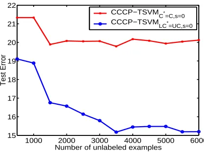
We also conducted an experiment to compare these two heuristics for larger unlabeled data sizes U . We took the sameuspstdata set (that is, the test part of the USPS data set) and we increased the number of unlabeled examples by adding up to 6000 additional unlabeled examples taken from the original USPS training set. Figure 6 reports the best test error for both heuristics over possible choices of γand C, taking the mean of the same 10 training splits with 50 labeled examples as before. The results indicate that C∗=C works poorly for large U .

(number of Coil20 g50c Text Uspst hyperparameters) CCCP-TSVM|s=0

C∗=C 22.33 4.68 7.76 20.09 2

CCCP-TSVM|s=0

UC∗=LC 16.69 5.62 7.97 16.57 2

CCCP-TSVM|s=0 _16.67 _4.56 _7.76 _16.55 ₃ CCCP-TSVM|C∗=C 19.02 4.28 5.22 18.33 3

CCCP-TSVM|UC∗=LC 16.06 5.04 5.59 16.47 3

CCCP-TSVM 15.92 3.92 4.92 16.45 4

Table 3: Comparison of C∗=C and C∗= _ULC heuristics on on Small-Scale Data Sets with the best optimized value of C∗(CCCP-TSVM|s=0_{or CCCP-TSVM, depending on whether s} is fixed). The heuristic C∗= L

UC maintains the balance between unlabeled points U and

labeled points L as U and L change, and is close to the best possible choice of C∗. The C∗=C heuristic also works for relatively small values of U as in this case. We report all methods with and without the optimization of s.

(14)

1000 2000 3000 4000 5000 6000 15

16 17 18 19 20 21 22

Number of unlabeled examples

Test Error

CCCP−TSVM

C*=C,s=0

CCCP−TSVM

LC*=UC,s=0

Figure 6: Comparison of the C∗=C and UC∗=LC heuristics on theuspstdata set as we increase the number of unlabeled examples by adding extra unlabeled data from the original usps training set. We report the best test error for both heuristics over possible of choices ofγ and C, taking the mean of the same 10 training splits with 50 labeled examples as before. As the number of unlabeled examples increases, the C∗ =C heuristic gives too much weight to the unlabeled data, resulting in no improvement in performance. Intuitively, the UC∗=LC heuristic balances the weight of the unlabeled and labeled data and empirically performs better.

also has a regularizing effect. The optimization is more likely to get stuck in a local minimum that appears when C∗ has a value much smaller than C. This may be why the C∗=C heuristic works well for algorithms that also use the annealing trick.

We conducted an experiment to see the performance of SVMLight-TSVM with and without the annealing heuristic. Ong50c, we chose a linear kernel and computed the optimal value of C on the test set using C∗=C. With the annealing heuristic, we obtain a test error of 7.6%. For the same parameters without the annealing procedure, we obtain 12.4%. Clearly the annealing heuristic has a strong effect on the results of SVMLight-TSVM. CCCP-TSVM has no such heuristic.

Effect of the parameter s The parameter s in CCCP-TSVM controls the choice of loss function to minimize over. It controls the size of the plateau of the Symmetric Ramp function (Figure 1, right). Training our algorithm with a tuned value of s appears to give slightly improved results over using the Symmetric Hinge loss (s=0, see Figure 1, left), especially on thetextdata set, as can be seen in Tables 2 and 3. Furthermore, Figure 7 highlights the importance of the parameter s of the loss function (2) by showing the best test error over different choices of s for two data sets,textand

g50c.

(15)

−15 −0.8 −0.6 −0.4 −0.2 0 7.5

10 12.5 15 17.5 20

s

Testing Error (%)

−14 −0.8 −0.6 −0.4 −0.2 0

4.5 5 5.5 6 6.5 7 7.5 8

Testing Error (%)

s

Figure 7: Effect of the parameter s of the Symmetric Ramp loss (see Figure 1 and equation (2) ) on thetext data set (left) and theg50cdata set (right). The peaked loss of the Symmetric Hinge function (s=0) forces early decisions for theβvariables and might lead to a poor local optimum. This effect then disappears as soon as we clip the loss.

In fact, the∇T SV M authors make a similar argument to explain why they prefer their algorithm over SVMLight: “(SVMLight) TSVM might suffer from the combinatorial nature of its approach. By deciding, from the very first step, the putative label of every point (even with low confidence), it may lose important degrees of freedom at an early stage and get trapped in a bad local minimum”. Here, the authors are refering to the way SVMLight TSVM has a discrete rather than continuous approach of assigning labels to unlabeled data. However, we think that the smoothed loss function of∇TSVM may help it to outperform the Symmetric Hinge loss of SVMLight TSVM, making it similar to the clipped loss when we use s<0. Indeed, the∇TSVM smoothed loss, exp(−3t2), has small gradients when t is close to 0.

A potential issue of the Symmetric Ramp loss is the fact that the gradient is exactly 0 for points lying on the plateau. Points are not updated at all in this region. This may be sub-optimal: if we are unlucky enough that all unlabeled points lie in this region, we perform no updates at all. Performing model selection on parameter s eliminates this problem. Alternatively, we could use a piece-wise linear loss with two different slopes for|f(x)|>s and for |f(x)|<s. Although it is possible to optimize such a loss function using CCCP, we have not evaluated this approach.

5. Large Scale Experiments

In this section, we provide experimental results on large scale experiments. Since other methods are intractable on such data sets, we only compare CCCP-TSVM against SVMs.

5.1 RCV1 Experiments

(16)

la-Method Train Unlabeled Parameters Test

size size Error

SVM 100 0 C=252.97,σ=15.81 16.61%

TSVM 100 500 C=2.597,C∗₌₁₀_,_s₌₋₀_.₂_,_σ₌₃_.₉₅ _11.99% TSVM 100 1000 C=2.597,C∗₌₁₀_,_s₌₋₀_.₂_,_σ₌₃_.₉₅ _11.67% TSVM 100 2000 C=2.597,C∗=10,s=−0.2,σ=3.95 11.47%

TSVM 100 5000 C=2.597,C∗₌₂_.₅₂₉₇_,_s₌₋₀_.₂_,_σ₌₃_.₉₅ 10.65% TSVM 100 10000 C=2.597,C∗₌₂_.₅₂₉₇_,_s₌₋₀_.₄_,_σ₌₃_.₉₅ _10.64% SVM 1000 0 C=25.297,σ=7.91 11.04%

TSVM 1000 500 C=2.597,C∗=10,s=−0.4,σ=3.95 11.09%

TSVM 1000 1000 C=2.597,C∗₌₂_.₅₂₉₇_,_s₌₋₀_.₄_,_σ₌₃_.₉₅ 11.06% TSVM 1000 2000 C=2.597,C∗₌₁₀_,_s₋₀_.₄₌_,_σ₌₃_.₉₅ _10.77% TSVM 1000 5000 C=2.597,C∗₌₂_.₅₂₉₇_,_s₌₋₀_.₂_,_σ₌₃_.₉₅ _10.81% TSVM 1000 10000 C=2.597,C∗₌₂₅_.₂₉₇₀_,_s₌₋₀_.₄_,_σ₌₃_.₉₅ 10.72%

Table 4: Comparing CCCP-TSVMs with SVMs on the RCV1 problem for different number of labeled and unlabeled examples. See text for details.

beled examples. For model selection we use a validation set with 2000 and 4000 labeled examples for the two experiments. The remaining 12754 examples were used as a test set.

We chose the parameter C and the kernel parameterγ(using an RBF kernel) that gave the best performance on the validation set. This was done by training a TSVM using the validation set as the unlabeled data. These values were then fixed for every experiment.

We then varied the number of unlabeled examples U , and reported the test error for each choice of U . In each case we performed model selection to find the parameters C∗and s. A selection of the results can be seen in Table 4.

The best result we obtained for 1000 training points was 10.58% test error, when using 10500 unlabeled points, and for 100 training points was 10.42% when using 9500 unlabeled points. Com-pared to the best performance of an SVM of 11.04% for the former and 16.61% for the latter, this shows that unlabeled data can improve the results on this problem. This is especially true in the case of few training examples, where the improvement in test error is around 5.5%. However, when enough training data is available to the algorithm, the improvement is only in the order of one percent.

(17)

0 2 4 6 8 10 12 14 0

500 1000 1500 2000 2500 3000 3500 4000 4500

number of unlabeled examples [k]

optimization time [sec]

1k training set

0 2 4 6 8 10 12 14

0 500 1000 1500 2000 2500 3000 3500 4000 4500

number of unlabeled examples [k]

optimization time [sec]

0.1k training set

Figure 8: Optimization time for the Reuters data set as a function of the number of unlabeled data. The algorithm was trained on 1,000 points (left) and on 100 points (right). The dashed lines represent a parabola fitted at the time measurements.

Method Training Unlabeled Parameters Test

size size Error

SVM 100 0 C=10,γ=0.0128 23.44% TSVM 100 2000 C∗=1, s=−0.1 16.81% SVM 1000 0 C=10,γ=0.0128 7.77% TSVM 1000 2000 C∗=5, s=−0.1 7.13% TSVM 1000 5000 C∗=1, s=−0.1 6.28% TSVM 1000 10000 C∗=0.5, s=−0.1 5.65% TSVM 1000 20000 C∗=0.3, s=−0.1 5.43% TSVM 1000 40000 C∗=0.2, s=−0.1 5.31% TSVM 1000 60000 C∗=0.1, s=−0.1 5.38%

Table 5: Comparing CCCP-TSVMs with SVMs on the MNIST problem for different number of labeled and unlabeled examples. See text for details.

5.2 MNIST Experiments

(18)

0 1 2 3 4 5 6 x 104 −10

0 10 20 30 40

Time (Hours)

Number of Unlabeled Examples CCCP−TSVM

Quadratic fit

Figure 9: Optimization time for the MNIST data set as a function of the number of unlabeled data. The algorithm was trained on 1,000 labeled examples and up to 60,000 unlabeled exam-ples. The dashed lines represent a polynomial of degree two with a least square fit on the algorithm’s time measurements.

more unlabeled data, we only reperformed model selection on C∗as it appeared that this parameter was the most sensitive to changes in the unlabeled set, and kept the other parameters fixed. For the larger labeled set we took 2000, 5000, 10000, 20000, 40000 and 60000 unlabeled examples. We always measure the error rate on the complete test set. The test error rate and parameter choices for each experiment are given in the Table 5, and the training times are given in Figure 9.

The results show an improvement over SVM for CCCP-TSVMs which increases steadily as the number of unlabeled examples increases. Most experiments in semi-supervised learning only use a few labeled examples and do not use as many unlabeled examples as described here. It is thus reassuring to know that these methods do not apply just to toy examples with around 50 training points, and that gains are still possible with more realistic data set sizes.

6. Discussion and Conclusions

TSVMs are not the only means of using unlabeled data to improve generalization performance on classification tasks. In the following we discuss some competing algorithms for utilizing unlabeled data, and also discuss the differences between the transductive and semi-supervised learning frame-works. Finally, we conclude with some closing remarks.

6.1 Cluster Kernels and Manifold-Learning

(19)

et al., 2002; Chapelle and Zien, 2005; Sindhwani et al., 2005; Szummer and Jaakkola, 2001b); and (Weston et al., 2003).

Other notable methods include generalizations of nearest-neighbor or Parzen window type ap-proaches to learning manifolds given labeled data (Zhu et al., 2003; Belkin and Niyogi, 2002; Zhou et al., 2004). Finally, Bayesian approaches have also been pursued (Graepel et al., 2000; Lawrence and Jordan, 2005).

We note that some cluster kernel methods (Chapelle and Zien, 2005) can perform significantly better than TSVM on some data sets. In fact, Chapelle and Zien (2005) show that, as these methods provide a new representation, one can just as easily run TSVM on the new representation. The combination of TSVM and cluster kernels then provides state-of-the-art results.

6.2 Semi-Supervised Versus Transductive Learning

From a theoretical point of view, there is much ideological debate over which underlying theory that explains TSVM is correct. The argument here is largely about which framework, semi-supervised learning or transductive, is interesting to study theoretically or to apply practically.

Semi-supervised school The majority of researchers appear to be in the semi-supervised school of thought, which claims that TSVMs help simply because of a regularizer that reflects prior knowl-edge, see e.g. (Chapelle and Zien, 2005). That is, one is given a set of unlabeled data, and one uses it to improve an inductive classifier to improve its generalization on an unseen test set.

Transductive school Vapnik (1982) describes transduction as a mathematical setup for describing learning algorithms that benefit from the prior knowledge of the unlabeled test patterns. Vapnik claims that transduction is an essentially easier task than first learning a general inductive rule and then applying it to the test examples. Transductive bounds address the performance of the trained system on these test patterns only. They do not apply to test patterns that were not given to the algorithm in the first place. As a consequence, transductive bounds are purely derived from combinatorial arguments (Vapnik, 1982) and are more easily made data-dependent (Bottou et al., 1994; Derbeko et al., 2004). Whether this is a fundamental property or a technical issue is a matter of debate.

Experiments The following experiments attempt to determine whether the benefits of TSVMs are solely caused by the prior knowledge represented by the distribution of the unlabeled data. If this is the case, the accuracy should not depend on the presence of the actual test patterns in the unlabeled data.

The following experiments consider three distinct subsets: a small labeled training set and two equally sized sets of unlabeled examples. Generalization accuracies are always measured on the third set. On the other hand, we run CCCP-TSVM using either the second or the third set as unlabeled data. We respectively name these results “Semi-Supervised TSVM” and “Transductive TSVM”. Experiments were carried out on both the Text and MNIST data set (class 8 vs rest) using ten splits. For Text, we fixed to a linear kernel, C=1000, and s=−0.3. For MNIST-8 we fixed

γ=0.0128 and C=10. We report the best test error over possible values of C∗. Table 6 shows that transductive TSVMs perform slightly better than semi-supervised TSVMs on these data sets.

(20)

Text MNIST-8

SVM 18.86% 6.68%

semi-supervised TSVM 6.60% 5.27% transductive TSVM 6.12% 4.87%

Table 6: Transductive TSVM versus Semi-Supervised TSVM.

6.3 Conclusion and Future Directions

In this article we have described an algorithm for TSVMs using CCCP that brings scalability im-provements over existing implementation approaches. It involves the iterative solving of standard dual SVM QP problems, and usually requires just a few iterations. One nice thing about being an extension of standard SVM training is that any improvements in SVM scalability can immediately also be applied to TSVMs. For example in the linear case, one could easily apply fast linear SVM training such as in (Keerthi and DeCoste, 2005) to produce very fast linear TSVMs. For the non-linear case, one could apply the online SVM training scheme of Bordes et al. (2005) to give a fast online transductive learning procedure.

Acknowledgments

We thank Hans Peter Graf, Eric Cosatto, and Vladimir Vapnik for their advice and support. Part of this work was funded by NSF grant CCR-0325463.

Appendix A. Derivation of the Optimization Problem

We consider a set of L training pairs

L

={(x1,y1), . . . ,(xL,yL)}, x∈Rn, y∈ {1,−1}and a

(un-labeled) set of U test vectors

U

={xL+1, . . . ,xL+U}. SVMs have a decision function fθ(.) of the

form

fθ(x) =w·Φ(x) +b,

whereθ= (w,b)are the parameters of the model, andΦ(·)is the chosen feature map.

We are interested in minimizing the TSVM cost function (3), under the constraint (4). We rewrite the problem here for convenience: minimizing

Js(θ) =1

2kwk

2₊_C

∑

L

i=1

∑

i=L+1

Rs(yifθ(xi)), (12)

under the constraint

1 U

L+U

∑

i=L+1

fθ(xi) =

1 L

L

∑

i=1

yi. (13)

Assume that a cost function J(θ) can be rewritten as the sum of a convex part Jvex(θ) and a

concave part Jcav(θ). As mentioned above in Algorithm 1, the minimization of J(θ)with respect to

θ(θbeing possibly restricted to a space

A

defined by some linear constraints) can be achieved by iteratively updating the parametersθusing the following update

θt+1=arg min

θ∈A

Jvex(θ) +Jcav′ (θt)·θ

(21)

In the case of our cost (12), we showed (see (9)) that Js(θ)can be decomposed into the sum of J_vexs (θ)and J_cavs (θ)where

J_vexs (θ) =1

2kwk

2₊_C

∑

L

i=1

H1(yi fθ(xi)) +C∗ L+2U

∑

i=L+1

H1(yi fθ(xi)) (15)

and

J_cavs (θ) =−C∗

L+2U

∑

i=L+1

Hs(yifθ(xi)). (16)

In order to apply the CCCP update (14) we first have to calculate the derivative of the concave part (16) with respect toθ:

∂J_cavs (θ)

∂θ =−C

∗L+

∑

2U

i=L+1

∂fθ(xi) ∂θ

We introduce the notation

βi=yi

=

C∗H_s′[yifθ(xi)] if i≥L+1

0 otherwise

=

C∗ if yifθ(xi)<s and i≥L+1

0 otherwise .

Since fθ(xi) =w·Φ(xi) +b withθ= (w,b), and∂fθ(xi)/∂θ= (Φ(xi),1), each update (14)

of the CCCP procedure applied to the our minimization problem (12) consists in minimizing the following cost

J_vexs (θ) +∂J

s cav(θ)

∂θ ·θ=J

s vex(θ) +

L+2U

∑

i=L+1

yiβi

∂fθ(xi) ∂θ

!

·θ

=J_vexs (θ) +

L+2U

∑

i=L+1

βiyi[w·Φ(xi) +b],

(17)

under the linear constraint (13).

The convex part (16) contains Hinge Losses which can be rewritten as

H1(z) =max(0,1−z) =minξ s.t ξ≥0,ξ≥1−z.

It is thus easy to see that the minimization of (17) under the constraint (13) is equivalent to the following quadratic minimization problem under constraints:

arg min

θ,ξ

1 2||w||

2₊_C

∑

L

i=1

ξi+C∗ L+2U

∑

i=L+1

ξi+ L+2U

∑

i=L+1

βiyifθ(xi)

s.t. 1 U

L+U

∑

i=L+1

fθ(xi) =

1 L

L

∑

i=1

yi (18)

yifθ(xi)≥1−ξi ∀1≤i≤L+2U (19)

(22)

Introducing Lagrangian variablesα0,αandν corresponding respectively to constraints (18), (19) and (20), we can write the Lagrangian of this problem as

L

(θ,ξ,α,ν) =1

2||w||

2₊_C

∑

L

i=1

ξi+C∗ L+2U

∑

i=L+1

ξi+ L+2U

∑

i=L+1

βiyi fθ(xi)

−α0 1 U

L+U

∑

i=L+1

fθ(xi)−

1 L

L

∑

i=1

yi

!

− L+2U

∑

i=1

αi(yifθ(xi)−1+ξi)

− L+2U

∑

i=1

νiξi,

(21)

whereα0can be positive or negative (equality constraint) andαi,i≥1 are non-negative (inequality

constraints).

Taking into account thatβi=0 for i≤L, calculating the derivatives with respect to the primal

variables yields

∂

L

∂w = w−

L+2U

∑

i=1

yi(αi−βi)Φ(xi)− α0

U

L+U

∑

i=L+1

Φ(xi)

∂

L

∂b = −

L+2U

∑

i=1

yi(αi−βi)−α0

∂

L

∂ξi

= C−αi−νi ∀1≤i≤L

∂

L

∂ξi

= C∗−αi−νi ∀L+1≤i≤L+2U.

For simplifying the notation, we now define an extra special examplex0in an implicit manner:

Φ(x0) = 1 U

L+U

∑

i=L+1

Φ(xi),

and we set y0=1 andβ0=0. Setting the derivatives to zero gives us

w=

L+2U

∑

i=0

yi(αi−βi)Φ(xi) (22)

and

L+2U

∑

i=0

yi(αi−βi) =0 (23)

and also

C−αi−νi=0 ∀1≤i≤L, C∗−αi−νi ∀L+1≤i≤L+2U. (24)

(23)

Lagrangian (21) yields the following maximization problem

arg max

α

−1

2

L+2U

∑

i,j=0

yiyj(αi−βi) (αj−βj)Φ(xi)·Φ(xj)

+

L+2U

∑

i=1

αi+α0 1 L

L

∑

i=1

yi

! (25)

under the constraints

0≤αi≤C ∀1≤i≤L

0≤αi≤C∗ ∀L+1≤i≤L+2U ∑L+2U

i=0 yi(αi−βi) =0.

(26)

The parameterwis then given by (22) and b is obtained using one of the following Karush-Kuhn-Tucker (KKT) conditions:

α06=0 =⇒ 1 U

L+U

∑

i=L+1

[w·Φ(xi) +b] =

1 L

L

∑

i=1

yi

∀1≤i≤L, 0<αi<C =⇒ yi[w·Φ(xi) +b] =1 ∀L+1≤i≤L+2U,0<αi<C∗ =⇒ yi[w·Φ(xi) +b] =1

If we defineζi=yifor 1≤i≤L+2U andζ0=_L1∑Li=1yi, and consider the kernel matrix K such

that

Ki j=Φ(xi)·Φ(xj),

and we perform the substitution

˜

αi=yi(αi−βi),

then we can rewrite the maximization problem (25) under the constraints (26) as the following

arg max ˜

α

ζ·α˜ −1

2α˜

T

K ˜α

under the constraints

0≤yiα˜i≤C ∀1≤i≤L

−βi≤yiα˜i≤C∗−βi ∀L+1≤i≤L+2U (27)

∑L+2U

i=0 α˜i=0.

Obviously this optimization problem is very close to an SVM optimization problem. It is thus possible to optimize it with a standard optimizer for SVMs. Note that only the bounds in (27) on the ˜αi have to be adjusted after each update ofβ.

References

(24)

K. Bennett and A. Demiriz. Semi-supervised support vector machines. In M. S. Kearns, S. A. Solla, and D. A. Cohn, editors, Advances in Neural Information Processing Systems 12, pages 368–374. MIT Press, Cambridge, MA, 1998.

T. De Bie and N. Cristianini. Convex methods for transduction. In S. Thrun, L. Saul, and B. Sch¨olkopf, editors, Advances in Neural Information Processing Systems 16. MIT Press, Cam-bridge, MA, 2004.

A. Bordes, S. Ertekin, J. Weston, and L. Bottou. Fast kernel classifiers with online and active learning. Journal of Machine Learning Research, May 2005. http://jmlr.csail.mit.edu/papers/v6/bordes05a.html.

B. E. Boser, I. M. Guyon, and V. N. Vapnik. A training algorithm for optimal margin classifiers. In Proceedings of the 5th Annual ACM Workshop on Computational Learning Theory, pages 144–152, Pittsburgh, PA, 1992. ACM Press.

L. Bottou, C. Cortes, and V. Vapnik. On the effective VC dimension. Technical Report bottou-effvc.ps.Z, Neuroprose (ftp://archive.cse.ohio-state.edu/pub/neuroprose), 1994.

O. Chapelle and A. Zien. Semi-supervised classification by low density separation. In Proceedings of the Tenth International Workshop on Artificial Intelligence and Statistics, 2005.

O. Chapelle, J. Weston, and B. Sch¨olkopf. Cluster kernels for semi-supervised learning. Neural Information Processing Systems 15, 2002.

R. Collobert, F. Sinz, J. Weston, and L. Bottou. Trading convexity for scalability. In ICML ’06: Proceedings of the 23rd international conference on Machine learning, pages 201–208, New York, NY, USA, 2006. ACM Press.

P. Derbeko, R. El-Yaniv, and R. Meir. Explicit learning curves for transduction and application to clustering and compression algorithms. Journal of Artificial Intelligence Research, 22:117–142, 2004.

G. Fung and O. Mangasarian. Semi-supervised support vector machines for unlabeled data clas-sification. In Optimisation Methods and Software, pages 1–14. Kluwer Academic Publishers, Boston, 2001.

T. Graepel, R. Herbrich, and K. Obermayer. Bayesian transduction. In Advances in Neural Infor-mation Processing Systems 12, NIPS, pages 456–462, 2000.

T. Joachims. Making large-scale support vector machine learning practical. In B. Sch¨olkopf, C. Burges, and A. Smola, editors, Advances in Kernel Methods. The MIT Press, 1999a.

T. Joachims. Transductive inference for text classification using support vector machines. In Inter-national Conference on Machine Learning, ICML, 1999b.

S. Keerthi and D. DeCoste. A modified finite newton method for fast solution of large scale linear svms. Journal of Machine Learning Research, 6:341–361, 2005.

(25)

N. Krause and Y. Singer. Leveraging the margin more carefully. In International Conference on Machine Learning, ICML, 2004.

N. D. Lawrence and M. I. Jordan. Semi-supervised learning via gaussian processes. In Advances in Neural Information Processing Systems, NIPS. MIT Press, 2005.

H. A. Le Thi. Analyse num´erique des algorithmes de l’optimisation D.C. Approches locales et globale. Codes et simulations num´eriques en grande dimension. Applications. PhD thesis, INSA, Rouen, 1994.

Y. LeCun, L. Bottou, G. B. Orr, and K.-R. M¨uller. Efficient backprop. In G.B. Orr and K.-R. M¨uller, editors, Neural Networks: Tricks of the Trade, pages 9–50. Springer, 1998.

D. D. Lewis, Y. Yang, T. Rose, and F. Li. Rcv1: A new benchmark collection for text categorization research. Journal of Machine Learning Research, 5:361–397, 2004. URLhttp://www.jmlr.

org/papers/volume5/lewis04a/lewis04a.pdf.

L. Mason, P. L. Bartlett, and J. Baxter. Improved generalization through explicit optimization of margins. Machine Learning, 38(3):243–255, 2000.

J. C. Platt. Fast training of support vector machines using sequential minimal optimization. In B. Sch¨olkopf, C. Burges, and A. Smola, editors, Advances in Kernel Methods. The MIT Press, 1999.

S.A.Nene, S.K.Nayar, and H.Murase. Columbia object image libary (coil-20). Technical Report CUS-005-96, Columbia Univ. USA, Febuary 1996.

B. Sch¨olkopf, A. Smola, and K.-R. M¨uller. Kernel principal component analysis. In Proceedings ICANN97, Springer Lecture Notes in Computer Science, page 583, 1997.

X. Shen, G. C. Tseng, X. Zhang, and W. H. Wong. On (psi)-learning. Journal of the American Statistical Association, 98(463):724–734, 2003.

V. Sindhwani, P. Niyogi, and M. Belkin. Beyond the point cloud: from transductive to semi-supervised learning. In International Conference on Machine Learning, ICML, 2005.

A. J. Smola, S. V. N. Vishwanathan, and T. Hofmann. Kernel methods for missing variables. In Proceedings of the Tenth International Workshop on Artificial Intelligence and Statistics, 2005.

M. Szummer and T. Jaakkola. Partially labeled classification with markov random walks. NIPS, 14, 2001a.

M. Szummer and T. Jaakkola. Partially labeled classification with Markov random walks. Neural Information Processing Systems 14, 2001b.

V. Vapnik. The Nature of Statistical Learning Theory. Springer, second edition, 1995.

(26)

J. Weston, C. Leslie, D. Zhou, A. Elisseeff, and W. S. Noble. Cluster kernels for semi-supervised protein classification. Advances in Neural Information Processing Systems 17, 2003.

L. Xu, J. Neufeld, B. Larson, and D. Schuurmans. Maximum margin clustering. In L. K. Saul, Y. Weiss, and L. Bottou, editors, Advances in Neural Information Processing Systems 17, pages 1537–1544. MIT Press, Cambridge, MA, 2005.

A. L. Yuille and A. Rangarajan. The concave-convex procedure (CCCP). In T. G. Dietterich, S. Becker, and Z. Ghahramani, editors, Advances in Neural Information Processing Systems 14, Cambridge, MA, 2002. MIT Press.

D. Zhou, O. Bousquet, T. N. Lal, J. Weston, and B. Sch¨olkopf. Learning with local and global consistency. In Advances in Neural Information Processing Systems, NIPS, 2004.