The Thirty-Third AAAI Conference on Artificial Intelligence (AAAI-19)
Object Detection Based on Region Decomposition and Assembly
Seung-Hwan Bae
Computer Vision Lab., Department of Computer Science and Engineering Incheon National University, 119 Academy-ro, Yeonsu-gu, Incheon, 22012, Korea
Abstract
Region-based object detection infers object regions for one or more categories in an image. Due to the recent advances in deep learning and region proposal methods, object detec-tors based on convolutional neural networks (CNNs) have been flourishing and provided the promising detection results. However, the detection accuracy is degraded often because of the low discriminability of object CNN features caused by occlusions and inaccurate region proposals. In this paper, we therefore propose a region decomposition and assembly de-tector (R-DAD) for more accurate object detection.
In the proposed R-DAD, we first decompose an object re-gion into multiple small rere-gions. To capture an entire appear-ance and part details of the object jointly, we extract CNN features within the whole object region and decomposed re-gions. We then learn the semantic relations between the object and its parts by combining the multi-region features stage by stage with region assembly blocks, and use the combined and high-level semantic features for the object classification and localization. In addition, for more accurate region proposals, we propose a multi-scale proposal layer that can generate ob-ject proposals of various scales. We integrate the R-DAD into several feature extractors, and prove the distinct performance improvement on PASCAL07/12 and MSCOCO18 compared to the recent convolutional detectors.
Introduction
Object detection is to find all the instances of one or more classes of objects given an image. In the recent years, the great progress of object detection have been also made by combining the region proposal algorithms and CNNs. The most notable work is the R-CNN (Girshick et al. 2014) framework. They first generate object region proposals us-ing the selective search (Uijlus-ings et al. 2013), extract CNN features (Krizhevsky, Sutskever, and Hinton 2012) of the re-gions, and classify them with class-specific SVMs. Then, Fast RCNN (Girshick 2015) improve the R-CNN speed us-ing feature sharus-ing and RoI poolus-ing. The recent detectors (Ren et al. 2015; Redmon et al. 2016; Liu et al. 2016) inte-grate the external region proposal modules into a CNN for boosting the training and detection speed further. As a re-sult, the detection accuracy can be also enhanced by joint learning of region proposal and classification modules.
Copyright c2019, Association for the Advancement of Artificial Intelligence (www.aaai.org). All rights reserved.
The modern convolutional detectors usually simplify fea-ture extraction and object detection processes with a fixed input scale. But even with the robustness of the CNNs to the scale variance, the region proposal accuracy is frequently degraded by the mismatches of produced proposals and ob-ject regions. Also, the mismatch tends to be increased for the small object detection (Lin et al. 2017a). To improve the proposal accuracy, multi-scale feature representation us-ing feature pyramid is used for generatus-ing stronger synthetic feature maps. However, featurizing each level of an image pyramid increases the inference time significantly. In an at-tempt to reduce the detection complexity, (Lin et al. 2017a) leverage the feature pyramid of CNNs.
In general, detections failures are frequently caused for occluded objects. In this case, the CNN feature discriminat-bility for the occluded one can be reduced considerably since the some part details of the object are missing in the oc-cluded regions. It implies that exploiting global appearance features for an entire object region could be insufficient to classify and localize objects accurately.
In this paper, we propose a novel region decomposition and assembly detector (R-DAD) to resolve the limitations of the previous methods. The proposed method is based on (1)multi-scale-based region proposalto improve region pro-posal accuracy of the region propro-posal network (RPN) and (2)
multi-region-based appearance modelto describe the global and part appearances of an object jointly.
In a multi-scale region proposal layer, we first generate region proposals using RPN and re-scale the proposals with different scaling factors to cover the variability of the object size. We then select the region proposals suitable for train-ing and testtrain-ing in considerations of the ratios of object and non-object samples to handle the data imbalanced problem. The main benefits of our method is that we can deal with the variability of the object size using the region scaling with-out expensive image or feature pyramids while maintaining the appropriate number of region proposals using the region sampling. In addition, we can capture local and global text cues by rescaling the region proposals. To be more con-crete, we can capture the local details with smaller proposals than its original region and the global context between object and surround regions with larger proposals.
combining features of an entire object and its parts. The main idea behind this method is that a maximum response from each feature map is a strong visual cue to identify ob-jects. However, we also need to learn the semantic relations
(i.e.weights) between the entire and decomposed regions for
combining them adaptively. For instance, when the left part of an object is occluded, the weights should be adjusted to be used features of the right part more for object detection since the features of the less occluded part are more reliable. To this end, we propose a region assembly block (RAB) for ensembling multi-region features. Using the RABs, we first learn the relations between part feature maps and gen-erate a combined feature map of part models by aggregat-ing maximum responses of part features stage-by-stage. We then produce strong high-level semantic features by combin-ing global appearance and part appearance features, and use them for classification and localization.
To sum up, the main contributions of this paper can be summarized as follows: (i) proposition of the R-DAD archi-tecture that can perform multi-scale-based region proposal and multi-region-based appearance learning through end-to-end training (ii) achievement of state-of-the-art results with-out employing other performance improvement methods
(e.g. feature pyramid, multi-scale testing, data
augmenta-tion, model ensemble, etc.) for several detection benchmark challenge on PASCAL07 (mAP of 81.2%), PASCAL12 (mAP of 82.0%), and MSCOCO18 (mAP of 43.1%) (iii) extensive implementation of R-DADs with various feature extractors and thorough ablation study to prove the effective-ness and robusteffective-ness of R-DAD. In this work, we first apply the proposed detection methods for the Faster RCNN (Ren et al. 2015), but we believe that our methods can be applied for other covolutional detectors (Girshick 2015; Bell et al. 2016; Kong et al. 2016; Dai et al. 2016) including RPN since these methods do not depend on a structure of a network.
Related Works
In spired of the recent advances in deep learning, a lot of progress has been made on object detection. In particular, convolutional detectors have become popular since it allows effective feature extraction and end-to-end training from im-age pixels to object classification and localization. In par-ticular, the remarkable improvement of deep networks for large scale object classification has also leaded to the im-provement of detection methods. For feature extraction and object classification, the recent object detectors are therefore constructed based on the deep CNNs (Simonyan and Zis-serman 2014; He et al. 2016) trained beforehand with large image datasets, and combined with region proposal and box regression networks for object localization. Among several works, Faster-RCNN (Ren et al. 2015) achieve the notice-able performance improvement by integrating RPN and Fast RCNN (Girshick 2015). In addition, (Redmon et al. 2016; Liu et al. 2016) develop the faster detectors by predicting object class and locations from feature maps directly with-out the region proposal stage.
For improving detection and segmentation, multiple fea-ture maps extracted from different resolutions and regions
have been exploited. (Gidaris and Komodakis 2015) im-prove the feature discriminability and diversity by combin-ing several region features. (Zeng et al. 2016) learn the rela-tion and dependency between feature maps of different reso-lutions via message passing. (Lin et al. 2017a) connect
con-volved and deconcon-volved (or up-sampled) feature mas from
bottom-up and top-down pathways for multi-scale feature representation. HyperNet (Kong et al. 2016) and ION (Bell et al. 2016) concatenate different layer feature maps, and then predict the objects with the transformed maps hav-ing more contextual and semantic information. Basically, the previous works based on multiple feature maps focus on (1) multi-region representation to improving the feature discriminability and diversity (2) multi-scale representation to detect the objects with small sizes without image pyra-mid. Although most previous detection methods with multi-ple features focus on only one of both issues, the proposed R-DAD can efficiently handle both issues together.
Region Decomposition and Assembly Detector
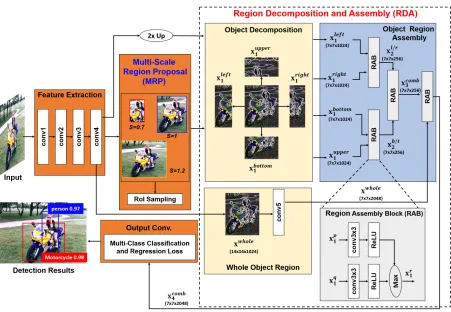
The architecture of our R-DAD is shown in Fig. 1. It mainly consists of feature extraction, multi-scale-based region pro-posal (MRP) and object region decomposition and assem-bly (RDA) phases. For extracting a generic CNN features, similar to other works, we use a classification network trained with ImageNet (Russakovsky et al. 2015). In our case, to prove the flexibility of our methods for the fea-ture extractors, we implement different detectors by com-bining our methods with several feature extractors: ZF-Net (Zeiler and Fergus 2014), VGG16/VGGM1024-Nets (Si-monyan and Zisserman 2014), Res-Net101/152 (He et al. 2016). In Table 3, we compare the detectors with different feature extractors. In Fig. 1, we however design the archi-tecture using ResNet as a base network.In the MRP network, we generate region proposals (i.e.
bounding boxes) of different sizes. By using the RPN (Ren et al. 2015), we first generate proposal boxes. We then re-scale the generated proposals with different re-scale factors for enhancing diversity of region proposals. In the RoI sampling layer, we select appropriate boxes among them for training and inference in consideration of the data balance between foreground and background samples.
In addition, we learn the global (i.e.an entire region) and
part appearance (i.e. decomposed regions) models in the
RDA network. The main process is that we decompose an entire object region into several small regions and extract features of each region. We then merge the several part mod-els while learning the strong semantic dependencies between decomposed parts. Finally, the combined feature maps be-tween part and global appearance models are used for object regression and classification.
Faster RCNN
We briefly introduce Faster-RCNN (Ren et al. 2015) since we implement our R-DAD on this framework. The detec-tion process of Faster-RCNN can be divided into two stages. In the first stage, an input image is resized to be fixed and
Figure 1: Proposed R-DAD architecture: In the MRP network, rescaled proposals are generated. For each rescaled proposal, we decompose it into several part regions. We design a region assembly block (RAB) with 3x3 convolution filters, ReLU, and max units. In the RDA network, by using RABs we combine the strong responses of decomposed object parts stage by stage, and then learn the semantic relationship between the whole object and part-based features.
network) such as VGG16 or ResNet. Then, the PRN uses
mid-level features at some selected intermediate level (e.g.
“conv4” and “conv5” for VGG and ResNet) for generating class-agnostic box proposals and their confidence scores.
In the second stage, features of box proposals are cropped by RoI pooling from the same intermediate feature maps used for box proposals. Since feature extraction for each pro-posal is simplified by cropping the extracted feature maps previously without the additional propagation, the speed can be greatly improved. Then, the features for box proposals are
subsequently propagated in other higher layers (e.g.“fc6”
followed by “fc7”) to predict a class and refine states (i.e.
locations and sizes) for each candidate box.
Multi-scale region proposal (MRP) network
Each bounding box can be denoted as d = (x, y, w, h),
where x, y, w and h are the center positions, width and
height. Given a region proposald, the rescaled box isds=
(x, y, w·s, h·s)with a scaling factors(≥0). By applying
differentsto the original box, we can generatedswith
dif-ferent sizes. Figure 2 shows the rescaled boxes with difdif-ferent
s, where the original boxdhass = 1. In our
implementa-tion, we use differents= [0.5,0.7,1,1.2,1.5].
Even though boxes with different scales can be generated
by the RPN in the Faster RCNN, we can further increase diversity of region proposals by using the multi-scale
detec-tion. By using largers, we can capture contextual
informa-tion (e.g. background or an interacting object) around the
object. On the other hand, by using smallerswe can
investi-gate local details in higher resolution and it can be useful for identifying the object under occlusion where the complete object details are unavailable. The effects of the multi-scale
proposals with differentsare shown in Table 1.
Since huge number of proposals (63×38×9×5) are
gen-erated for the feature maps of size63×38at the “conv4”
layer when using 9 anchors and 5 scale factors, exploiting all the proposals for training a network is impractical. Thus, we
maintain the appropriate number of proposals (e.g.256) by
removing the proposals with low confidence and low over-lap ratios over ground truth. We then make a ratio of object and non-object samples in a mini-batch to be equal and use the mini-batch for fine-tuning a detector shown in Fig 1.
Region decomposition and assembly (RDA)
network
Figure 2: (Left) Rescaled proposals by the MRP. (Right) Several decomposed regions for a whole object region.
the MRP network, we therefore infer strong cues by com-bining features of multiple regions stage-by-stage as shown in Fig. 1. To this end, we need to learn the weights which can represent semantic relations between the features of dif-ferent parts, and using the weights we control the amount of features to be propagated in the next layer.
A region proposal from RPN is assumed usually to cover the whole region of an object. We generate smaller
decom-posed regions by divingdinto several part regions. We make
the region cover different object parts as shown in Fig. 2. From the feature map used as the input of the MRP
network, we first extract the warped features xl of size
hroi×wroifor the whole object region using RoI pooling
(Girshick 2015), wherehroiandwroiare the height and the
width of the map (for ResNet,hroi = 14andwroi = 14).
Before extracting features of each part, we first upsample the spatial resolution of the feature map by a factor of 2 us-ing bilinear interpolation. We found that these finer resolu-tion feature maps improve the detecresolu-tion rate since the ob-ject details can be captured more accurately as shown in Table 1. Using RoI pooling, we also extract warped fea-ture maps of sizedhroi/2e × dwroi/2e, and denote them as
xpl, p∈ {left, right, bottom, upper}.
In the forward propagation, we convolve part features
xpi,l−1at layerl−1of sizehpl−1×wlp−1with different kernels
wijl of sizeml×ml, and then pass the convolved features
a nonlinear activation function f(·) to obtain an updated
feature mapxpj,lof size(hpl−1−ml+1)×(wpl−1−ml+1)as
xpj,l=fPkl
i=1x
p i,l−1∗w
l ij+blj
, l= 2, 3, 4 (1)
where p represent each part (left, right, bottom, upper)
or combined parts (left-right(l/r), bottom-upper (b/u) and
comb) as in Fig. 1.blj is a bias factor,klis the number of
kernels.∗means convolution operation. We use the
element-wise ReLU function asf(·)for scaling the linear input.
Then, the bi-directional outputsxpl andxql Eq. (1) of dif-ferent regions are merged to produce the combined feature
xr
l by using an element-wise max unit over each channel as
xr
l =max(x
p l,x
q
l) (2)
p,q andr also represent each part or a combined part as
shown in Fig. 2. The element-wise max unit is used to merge
information between xpl and xql and producexr
l with the
same size. As a result, the bottom-up feature maps are fined state-by-stage by comparing features of different re-gions and strong semantics features remained only. The holistic feature of the object is propagated through several
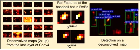
Figure 3: Intermediate semantic features and detection re-sults generated by our R-DAD.
layers (in “conv5 block” for ResNet) of the base network,
and the featuresxwhole for the whole object appearance at
the last layer is also compared with the combined feature
xcomb
3 of part models, and then the refined featuresxcomb4 are
connected with the object classification and box regression
layers withcls+ 1neurons and4(cls+ 1)neurons, where
clsis the number of object classes and the one is added due
to the background class.
Figure 3 shows the semantic features at several layers of the learned R-DAD. Some strong feature responses within objects are extracted by our R-DAD.
R-DAD Training
For training our R-DAD, we exploit the pre-trained and
shared parameters of a feature extractor (e.g.“conv1-5” of
ResNet) from the ImageNet dataset as initial parameters of R-DAD. We then fine-tune parameters of higher lay-ers (“conv3-5”) of the R-DAD while keeping parametlay-ers
of lower layers (e.g.“conv1-2”). We freeze the parameters
for batch normalization which was learned during ImageNet pre-training. The parameters of the MRP and RDA networks are initialized with the Gaussian distribution.
For each box d, we find the best matched ground truth
box d∗ by evaluating IoU. If a boxdhas an IoU than 0.5
with anyd∗, we assign positive labelo∗ ∈ {1...cls}, and
a vector representing the 4 parameterized coordinates ofd∗.
We assign a negative label (0) todthat has an IoU between
0.1 and 0.5. From the output layers of the R-DAD, 4
pa-rameterized coordinates and the class labeloˆare predicted
to each boxd. The adjusted boxdˆis generated by applying
the predicted regression parameters. For box regression, we use the following parameterization (Girshick et al. 2014).
tx= (ˆx−x)/w, ty= (ˆy−y)/h, tw=log( ˆw/w), th=log(ˆh/h),
(3)
whereˆxandxare for the predicted and anchor box,
respec-tively (likewise fory,w,h). Similarly,t∗ = [t∗x, t∗y, t∗w, t∗h]
is evaluated with the predicted box and ground truth boxes. We then train the R-DAD by minimizing the classification and regression losses Eq.(4).
L(o,o∗,t,t∗) =Lcls(o,o∗) +λ[o≥1]Lreg(t,t∗) (4) Lcls(o,o∗) =−Puδ(u, o∗)log(pu), (5)
Lloc(t,t∗) =−Pv∈{x,y,w,h}smoothL1(tv, t
∗
Table 1: Ablation study: effects of the proposed methods.
Method Combination
Multi-scale region proposal √ √ s= [0.7,1.0,1.5]
Multi-scale region proposal √ √ √
s= [0.5,0.7,1.0,1.2,1.5]
Decomposition/assembly √ √ √ √
Up-sampling √
Mean AP 68.90 70.0 70.30 71.95 72.65 73.90 74.90
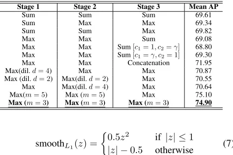
Table 2: Ablation study: the detection comparison of differ-ent region assembly blocks.
Stage 1 Stage 2 Stage 3 Mean AP
Sum Sum Sum 69.61
Sum Max Max 69.34
Sum Sum Max 69.82
Max Max Sum 69.08
Max Max Sum[c1= 1, c2=γ] 68.80
Max Max Sum[c1=γ, c2= 1] 69.30
Max Max Concatenation 71.95
Max(dil.d= 4) Max Max 70.87
Max (dil.d= 2) Max(dil.d= 2) Max 70.55
Max Max(dil.d= 4) Max 70.64
Max(m= 5) Max (m= 5) Max 75.10
Max (m= 3) Max (m= 3) Max (m= 3) 74.90
smoothL1(z) =
0.5z2 if |z| ≤1
|z| −0.5 otherwise (7)
wherepuis the predicted classification probability for class
u.δ(u, o∗) = 1ifu=o∗andδ(u, o∗) = 0otherwise. Using the SGD with momentum of 0.9, we train the parameters.
λ= 1in our implementation.
Discussion of R-DAD
There are several benefits of the proposed object region assembly method. Since we extract maximum responses across spatial locations between feature maps of object parts, we can improve the spatial invariance more to feature posi-tion without a deep hierarchy than using max pooling which
supports a small region (e.g.2×2). Since our RAB is
sim-ilar to the maxout unit except for using ReLU, the RAB can be used as a universal approximator which can approximate arbitrary continuous function (Goodfellow et al. 2013). This indicates that a wide variety of object feature configurations can be represented by combining our RABs hierarchically. In addition, the variety of region proposals generated by the MRP network can improve the robustness further to feature variation occurred by the spatial configuration change be-tween objects.
Implementation
We apply our R-DAD for various feature extractors to show its flexibility to the base network. In general, a feature ex-tractor affects the accuracy and speed of a detectors. In this work, we use five different feature extractors and combine each extractor with our R-DAD to compare each other as shown in Table 3 and 4. We implement all the detectors us-ing the Caffe on a PC with a sus-ingle TITAN Xp GPU without parallel and distributed training.
Table 3: Comparison between the R-DAD and Faster-RCNN by using different feature extractors on the VOC07 test set.
Train set Detector mAP Train set Detector mAP
FRCN/ZF 60.8 FRCN/ZF 66.0
R-DAD/ZF 63.7 R-DAD/ZF 68.2
PASCAL FRCN/VGGM1024 61.0 PASCAL FRCN/VGGM1024 65.0 VOC R-DAD/VGGM1024 65.0 VOC R-DAD/VGGM1024 69.1 07 FRCN/VGG16 69.9 07++12 FRCN/VGG16 73.2
R-DAD/VGG16 73.9 R-DAD/VGG16 78.2
FRCN/Res101 74.9 FRCN/Res101 76.6
R-DAD/Res101 77.6 R-DAD/Res101 81.2
ZF and VGG networks
We use the fast version of ZF (Zeiler and Fergus 2014) with 5 shareable convolutional and 3 fully-connected layers. We also use the VGG16 (Simonyan and Zisserman 2014) with 13 shareable convolutional and 3 fully connected layers. Moreover, we exploit the VGGM1024 (variant of VGG16) with the same depth of AlexNet (Krizhevsky, Sutskever, and Hinton 2012). All these models pre-trained with the ILSVRC classification dataset are given by (Ren et al. 2015).
To generate region proposals, we feed the feature maps of the last shared convolutional layer (“conv5” for ZF and VGGM1024, and “conv5 3” for VGG-16) to the MRP net-work. Given a set of region proposals, we also feed the shared maps of the last layer to the RDA network for learn-ing high-level semantic features by combinlearn-ing the features
of decomposed regions. We usexcomb
4 produced by the RDA
network as inputs of regression and classification layers. We fine-tune all layers of ZF and VGG1024, and conv3 1 and up for VGG16 to compare our R-DAD with Faster RCNN (Ren et al. 2015). The sizes of a mini-batch used for training MRP and RAD networks are set to 256 and 64, respectively.
Residual networks
We use the ResNets (He et al. 2016) with different depths by stacking different number of residual blocks. For the ResNets50/101/152 (Res50/101/152), the layers from “conv1” to “conv4” blocks are shared in the Faster RCNN. In a similar manner, we use the features from the last layer of the “conv4” block as inputs of the MRP and RDA networks. We fine-tune the layers of MRP and RDA networks includ-ing layers of “conv3-5” while freezinclud-ing layers of “conv1-2” layers. We also use the same mini-batch sizes (256/64) when training MRP and RDA networks per iteration.
Experimental results
We train and evaluate our R-DAD on standard detection benchmark datasets: PASCAL VOC07/12 (Everingham et al. 2015) and MSCOCO18 (Lin et al. 2014) datasets.
Table 4: The speed of the Faster R-CNN (FRCN) and R-DAD (input size: 600×1000).
Base Network ZF VGGM1024 VGG16 Res101 Res152
Detector FRCN R-DAD FRCN R-DAD FRCN R-DAD FRCN R-DAD R-DAD(m= 5) FRCN R-DAD R-DAD(m= 5) Time(sec/frame) 0.041 0.048 0.046 0.054 0.15 0.177 0.208 0.245 0.53 0.301 0.385 0.574
Table 5: Performance comparison with other detectors in PASCAL VOC 2012 challenge. The more results can be found in the PASCAL VOC 2012 website.
Train set Detector mAP aero bike bird boat bottle bus car cat chair cow table dog horse mbike person plant sheep sofa train tv Fast (Girshick 2015) 68.4 82.3 78.4 70.8 52.3 38.7 77.8 71.6 89.3 44.2 73.0 55.0 87.5 80.5 80.8 72.0 35.1 68.3 65.7 80.4 64.2 Faster (Ren et al. 2015) 70.4 84.9 79.8 74.3 53.9 49.8 77.5 75.9 88.5 45.6 77.1 55.3 86.9 81.7 80.9 79.6 40.1 72.6 60.9 81.2 61.5 PASCAL SSD512 (Liu et al. 2016) 74.9 87.4 82.3 75.8 59.0 52.6 81.7 81.5 90.0 55.4 79.0 59.8 88.4 84.3 84.7 83.3 50.2 78.0 66.3 86.3 72.0 VOC YOLOv2 (Redmon and Farhadi 2017) 73.4 86.3 82.0 74.8 59.2 51.8 79.8 76.5 90.6 52.1 78.2 58.5 89.3 82.5 83.4 81.3 49.1 77.2 62.4 83.8 68.7 07++12 MR-CNN (Gidaris and Komodakis 2015) 73.9 85.5 82.9 76.6 57.8 62.7 79.4 77.2 86.6 55.0 79.1 62.2 87.0 83.4 84.7 78.9 45.3 73.4 65.8 80.3 74.0 HyperNet (Kong et al. 2016) 71.4 84.2 78.5 73.6 55.6 53.7 78.7 79.8 87.7 49.6 74.9 52.1 86.0 81.7 83.3 81.8 48.6 73.5 59.4 79.9 65.7 ION (Bell et al. 2016) 76.4 87.5 84.7 76.8 63.8 58.3 82.6 79.0 90.9 57.8 82.0 64.7 88.9 86.5 84.7 82.3 51.4 78.2 69.2 85.2 73.5 R-DAD/Res101 80.2 90.0 86.6 81.3 71.2 66.0 83.4 83.7 94.5 63.2 84.0 64.2 92.8 90.1 88.6 87.3 62.2 82.8 70.9 88.8 72.2 R-DAD/Res152 82.0 90.2 88.1 85.3 73.3 71.4 84.5 87.4 94.6 65.1 86.8 64.0 94.1 89.7 89.2 89.3 64.5 83.5 72.2 89.5 77.6
Learning strategy: We use different learning rates for
each evaluation. We use a learning rateµ= 1e−3for 50k
it-erations, andµ= 1e−4for the next 20k iterations on VOC07
evaluation. For VOC12 evaluation, we train a detector with
µ = 1e−3 for 70k iterations, and continue it for 50k
iter-ations with µ = 1e−4. For MSCOCO evaluation, we use
µ= 1e−4andµ= 1e−5for the first 700k and the next 500k
iterations.
Ablation experiments
To show the effectiveness of the methods used for MRP and RDA networks, we perform several ablation studies. For this evaluation, we train detectors with VOC07+(trainval) set and test them on the VOC07 test set.
Effects of proposed methods:In Table. 1, we first show mAPs of a baseline detector without the multi-scale and
re-gion decomposition/assembly methods (i.e. Faster RCNN)
and the detector by using the proposed methods. Compared to the mAP of the baseline, we achieve the better rates when applying our methods. We also compare mAP of detec-tors with different number of scaling facdetec-tors. By using five scales, mAP is improved slightly. In particular, using
decom-position/assembly method can improve mAP to3.05%.
Us-ing up-samplUs-ing improves mAP to1%. This indicates that
part features extracted in finer resolution yield the better de-tection. As a result, combining all proposed methods with the baseline enhances the mAP to 6%.
Structure of the RDA network: To determine the best structure of the RDA network, we evaluate mAP by chang-ing its components as shown in Table 2. We first compare feature aggregation methods. As in Fig. 1, we combine the bi-directional outputs of different regions at each stage us-ing a max unit. We change this unit one-by-one with sum or concatenation units. When summing both outputs at the stage 3, we try to merge outputs with different coefficients.
Sum [c1 = γ, c2 = 1] means that xwhole andxcomb3 are
summed withγand 1 weights. This is a similar concept to
the identity mapping (He et al. 2016). The scale parameterγ
is learned during training. However, we found that summing feature maps or using identity mapping show the minor im-provement. In addition, concatenating features improves the mAP, but it also increases the memory usage and complexity
Figure 4: Comparisons of R-DAD without (top) /with (bot-tom) the RDA method under occlusions on COCO18.
of convolution at the next layer. From this comparison, we verify that merging the features using the max units for all the stages provides the best mAP while the computational complexity. This evaluation supports that our main idea of that maximum responses of features are strong visual cues for detecting objects.
Moreover, to determine the effective receptive field size,
we change the size of convolution kernels with m = 5at
the stage 1 and 2 in the RDA network. Moreover, we also
tryd-dilated convolution filters to expand the receptive field
more. However, exploiting the dilated convolutions and 5x5 convolution filters does not increase the mAP significantly. It indicates that we can cover the receptive fields of each part and combined regions sufficiently with the 3x3 filters.
Comparison with Faster-RCNN
Accuracy:To compare the Faster-RCNN (FRCN), we train
both detectors with the VOC07trainval (VOC07, 5011
im-ages) and VOC12trainval sets (VOC07++12, 11540
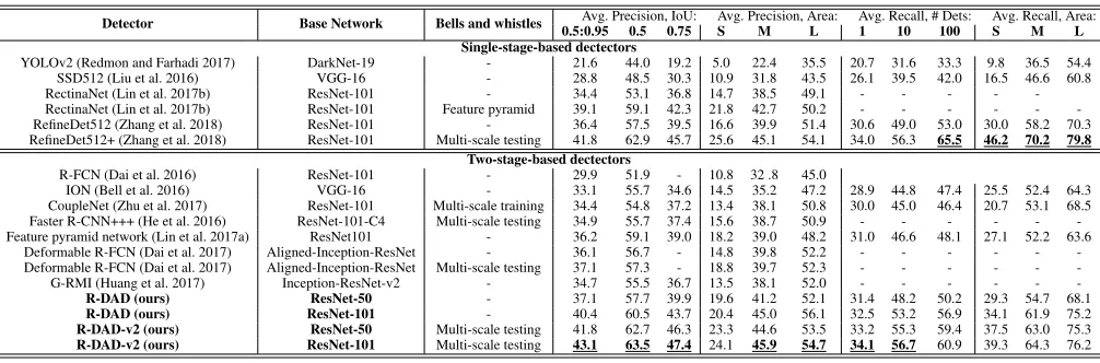
Table 6: Comparison of state-of-the-art detectors on MSCOCO18 test-dev set. More results can be founded in the MSCOCO evaluation website (test-dev2018). For each metric, the best results are underlined.
Detector Base Network Bells and whistles 0.5:0.95Avg. Precision, IoU:0.5 0.75 SAvg. Precision, Area:M L Avg. Recall, # Dets:1 10 100 Avg. Recall, Area:S M L Single-stage-based dectectors
YOLOv2 (Redmon and Farhadi 2017) DarkNet-19 - 21.6 44.0 19.2 5.0 22.4 35.5 20.7 31.6 33.3 9.8 36.5 54.4 SSD512 (Liu et al. 2016) VGG-16 - 28.8 48.5 30.3 10.9 31.8 43.5 26.1 39.5 42.0 16.5 46.6 60.8 RectinaNet (Lin et al. 2017b) ResNet-101 - 34.4 53.1 36.8 14.7 38.5 49.1 - - - - -RectinaNet (Lin et al. 2017b) ResNet-101 Feature pyramid 39.1 59.1 42.3 21.8 42.7 50.2 - - - -RefineDet512 (Zhang et al. 2018) ResNet-101 - 36.4 57.5 39.5 16.6 39.9 51.4 30.6 49.0 53.0 30.0 58.2 70.3 RefineDet512+ (Zhang et al. 2018) ResNet-101 Multi-scale testing 41.8 62.9 45.7 25.6 45.1 54.1 34.0 56.3 65.5 46.2 70.2 79.8
Two-stage-based dectectors
R-FCN (Dai et al. 2016) ResNet-101 - 29.9 51.9 - 10.8 32 .8 45.0
ION (Bell et al. 2016) VGG-16 - 33.1 55.7 34.6 14.5 35.2 47.2 28.9 44.8 47.4 25.5 52.4 64.3 CoupleNet (Zhu et al. 2017) ResNet-101 Multi-scale training 34.4 54.8 37.2 13.4 38.1 50.8 30.0 45.0 46.4 20.7 53.1 68.5 Faster R-CNN+++ (He et al. 2016) ResNet-101-C4 Multi-scale testing 34.9 55.7 37.4 15.6 38.7 50.9 - - - -Feature pyramid network (Lin et al. 2017a) ResNet101 - 36.2 59.1 39.0 18.2 39.0 48.2 31.0 46.6 48.1 27.1 52.2 63.6
Deformable R-FCN (Dai et al. 2017) Aligned-Inception-ResNet - 36.1 56.7 - 14.8 39.8 52.2 - - - -Deformable R-FCN (Dai et al. 2017) Aligned-Inception-ResNet Multi-scale testing 37.1 57.3 - 18.8 39.7 52.3 - - - -G-RMI (Huang et al. 2017) Inception-ResNet-v2 - 34.7 55.5 36.7 13.5 38.1 52.0 - - -
-R-DAD (ours) ResNet-50 - 37.1 57.7 39.9 19.6 41.2 52.1 31.4 48.2 50.2 29.3 54.7 68.1
R-DAD (ours) ResNet-101 - 40.4 60.5 43.7 20.4 45.0 56.1 32.5 53.2 56.9 34.1 61.9 75.2
R-DAD-v2 (ours) ResNet-50 Multi-scale testing 41.8 62.7 46.3 23.3 44.6 53.5 33.2 55.3 59.4 37.5 63.0 75.3
R-DAD-v2 (ours) ResNet-101 Multi-scale testing 43.1 63.5 47.4 24.1 45.9 54.7 34.1 56.7 60.9 39.3 64.3 76.2
mAP about 3∼5% using R-DAD. We also confirm that
us-ing feature extractors with higher classification accuracies leads to better detection rate.
Speed:In Table 4, we have compared the detection speed of both detectors. Since the speed depends on size of the base network, we evaluate them by using various base net-works. We also fix the number of region proposals to 300 as done in (Girshick 2015). The speed of our R-DAD is com-parable with it of the FRCN. Indeed, to reduce the detec-tion complexity while maintaining the accuracy, we design the R-DAD structure in consideration of several important factors. We found that the spatial sizes of RoI feature maps (hroi and wroi) and convolution filters (m) can affect the
speed significantly. When usinghroi = 14,wroi = 14and
m = 5 in RABs, R-DAD gets 1.5x∼2.1x slower but
en-hanced only about 0.2% as in Table 2. Therefore, we confirm that adding MRP and RDA networks to the Faster RCNN does not increase the complexity significantly.
Detection Benchmark Challenges
In this evaluation, our R-DAD performance is evaluated from PASCAL VOC and MSCOCO servers. We also post our detection scores to the leaderboard of each challenge.
PASCAL VOC 2012 challenge:We evaluate our R-DAD on the PASCAL VOC 2012 challenge. For training our R-DAD, we use VOC07++12 only and test it on VOC2012test (10911 images). Note that we do not use extra datasets such as the COCO dataset for improving mAP as done in many top ranked teams.
Table 5 shows the results. As shown, we achieve the best mAP among state-of-the-art convolutional detectors. In ad-dition, our detector shows the higher mAP by using the Res152 model. Compared to the Faster RCNN and MR-CNN (Gidaris and Komodakis 2015) using multi-region ap-proach, we improve the mAP to 11.6% and 8.1%.
MS Common Objects in Context (COCO) 2018 chal-lenge:We participate in the MSCOCO challenge. This chal-lenge is detection for 80 object categories. We use
COCO-style evaluation metrics: mAP averaged for IoU ∈ [0.5 :
0.05 : 0.95], average precision/recall on small (S), medium
(M) and large (L) objects, and average recall on the number
of detections (# Dets). We train our R-DAD with the union of train and validation images (123k images). We then test it on the test-dev set (20k images). For enhancing detection for the small objects, we use 12 anchors consisting of 4 scales (64, 128, 256, 512) and 3 aspect ratios (1:1, 1:2, 2:1).
Table 6 compares the performance of detectors based on a single network. We divide detectors with single-stage-based and two-stage-based detectors depending on region proposal approach. Note that our R-DAD with ResNet-50 is superior to other detectors. The performance of R-DAD is further im-proved to 40.4% by using ResNet-101 with higher accuracy. Compared to the scores of this challenge winners of Faster R-CNN+++ (2015) and G-RMI (2016), our detectors pro-duce the better results. Remarkably, we achieve the best
scores without bell and whistles (e.g. multi-scale testing,
hard example mining, feature pyramid (Lin et al. 2017a), model ensemble, etc). By applying multi-scale testing for R-DADs with ResNet50 and ResNet101, we can improve mAP to 41.8% and 44.9%, respectively. As shown in this chal-lenge leaderboard, our R-DAD is ranked on the high place.
In Fig. 4, we have directly compared detection results with/without the RDA network. Some detection failures (in-accurate localizations and false positives) for occluded ob-jects are occurred when not using the proposed network.
Conclusion
compari-son with other state-of-the-art convolutional detectors, we have proved that the proposed methods lead to the notice-able performance improvements on several benchmark chal-lenges such as PASCAL VOC07/12, and MSCOCO18. We clearly show that the robustness and flexibility of our meth-ods by implementing several versions of R-DADs with dif-ferent feature extractors and detection methods through ab-lation studies.
Acknowledgement
This work was supported by the National Research Founda-tion of Korea (NRF) grant funded by the Korea government (MSIT) (No. NRF-2018R1C1B6003785).
References
Bell, S.; Zitnick, C. L.; Bala, K.; and Girshick, R. B. 2016. Inside-outside net: Detecting objects in context with skip pooling and re-current neural networks. InCVPR, 2874–2883.
Dai, J.; Li, Y.; He, K.; and Sun, J. 2016. R-FCN: object detection via region-based fully convolutional networks. InNIPS, 1–9. Dai, J.; Qi, H.; Xiong, Y.; Li, Y.; Zhang, G.; Hu, H.; and Wei, Y. 2017. Deformable convolutional networks. InICCV, 764–773. Everingham, M.; Eslami, S. M. A.; Van Gool, L.; Williams, C. K. I.; Winn, J.; and Zisserman, A. 2015. The pascal visual ob-ject classes challenge: A retrospective.IJCV111(1):98–136. Gidaris, S., and Komodakis, N. 2015. Object detection via a multi-region and semantic segmentation-aware cnn model. In ICCV, 1134–1142.
Girshick, R. B.; Donahue, J.; Darrell, T.; and Malik, J. 2014. Rich feature hierarchies for accurate object detection and semantic seg-mentation. InCVPR, 580–587.
Girshick, R. B. 2015. Fast R-CNN. InICCV, 1440–1448. Goodfellow, I. J.; Warde-Farley, D.; Mirza, M.; Courville, A. C.; and Bengio, Y. 2013. Maxout networks. InICML, 1319–1327. He, K.; Zhang, X.; Ren, S.; and Sun, J. 2016. Deep residual learn-ing for image recognition. InCVPR, 770–778.
Huang, J.; Rathod, V.; Sun, C.; Zhu, M.; Korattikara, A.; Fathi, A.; Fischer, I.; Wojna, Z.; Song, Y.; Guadarrama, S.; and Murphy, K. 2017. Speed/accuracy trade-offs for modern convolutional object detectors. InCVPR, 7310–7319.
Kong, T.; Yao, A.; Chen, Y.; and Sun, F. 2016. Hypernet: Towards accurate region proposal generation and joint object detection. In CVPR, 845–853.
Krizhevsky, A.; Sutskever, I.; and Hinton, G. E. 2012. Imagenet classification with deep convolutional neural networks. InNIPS, 1106–1114.
Lin, T.; Maire, M.; Belongie, S. J.; Bourdev, L. D.; Girshick, R. B.; Hays, J.; Perona, P.; Ramanan, D.; Doll´ar, P.; and Zitnick, C. L. 2014. Microsoft COCO: common objects in context. CoRR abs/1405.0312.
Lin, T.; Doll´ar, P.; Girshick, R. B.; He, K.; Hariharan, B.; and Be-longie, S. J. 2017a. Feature pyramid networks for object detection. InCVPR, 936–944.
Lin, T.; Goyal, P.; Girshick, R. B.; He, K.; and Doll´ar, P. 2017b. Focal loss for dense object detection. InICCV, 2999–3007. Liu, W.; Anguelov, D.; Erhan, D.; Szegedy, C.; Reed, S. E.; Fu, C.; and Berg, A. C. 2016. SSD: single shot multibox detector. In ECCV, 21–37.
Redmon, J., and Farhadi, A. 2017. YOLO9000: better, faster, stronger. InCVPR, 6517–6525.
Redmon, J.; Divvala, S. K.; Girshick, R. B.; and Farhadi, A. 2016. You only look once: Unified, real-time object detection. InCVPR, 779–788.
Ren, S.; He, K.; Girshick, R. B.; and Sun, J. 2015. Faster R-CNN: towards real-time object detection with region proposal networks. InNIPS, 91–99.
Russakovsky, O.; Deng, J.; Su, H.; Krause, J.; Satheesh, S.; Ma, S.; Huang, Z.; Karpathy, A.; Khosla, A.; Bernstein, M.; Berg, A. C.; and Fei-Fei, L. 2015. ImageNet Large Scale Visual Recognition Challenge.IJCV115(3):211–252.
Simonyan, K., and Zisserman, A. 2014. Very deep convolutional networks for large-scale image recognition.CoRRabs/1409.1556. Uijlings, J. R. R.; van de Sande, K. E. A.; Gevers, T.; and Smeul-ders, A. W. M. 2013. Selective search for object recognition.IJCV 104(2):154–171.
Zeiler, M. D., and Fergus, R. 2014. Visualizing and understanding convolutional networks. InECCV, 818–833.
Zeng, X.; Ouyang, W.; Yan, J.; Li, H.; Xiao, T.; Wang, K.; Liu, Y.; Zhou, Y.; Yang, B.; Wang, Z.; Zhou, H.; and Wang, X. 2016. Crafting gbd-net for object detection.CoRRabs/1610.02579. Zhang, S.; Wen, L.; Bian, X.; Lei, Z.; and Li, S. Z. 2018. Single-shot refinement neural network for object detection. CVPR4203– 4212.