Hypergraph Neural Networks

The Thirty-Third AAAI Conference on Artificial Intelligence (AAAI-19)

Hypergraph Neural Networks

Yifan Feng,

Haoxuan You,

Zizhao Zhang,

Rongrong Ji,

Yue Gao

School of Information Science and Engineering, Xiamen University, 361005, China 2_{Peng Cheng Laboratory, China}

3_{BNRist, KLISS, School of Software, Tsinghua University, 100084, China.}

{evanfeng97, haoxuanyou}@gmail.com, [email protected],{zz-z14,gaoyue}@tsinghua.edu.cn

Abstract

In this paper, we present a hypergraph neural networks (HGNN) framework for data representation learning, which can encode high-order data correlation in a hypergraph struc-ture. Confronting the challenges of learning representation for complex data in real practice, we propose to incorpo-rate such data structure in a hypergraph, which is more flexi-ble on data modeling, especially when dealing with complex data. In this method, a hyperedge convolution operation is designed to handle the data correlation during representation learning. In this way, traditional hypergraph learning proce-dure can be conducted using hyperedge convolution opera-tions efficiently. HGNN is able to learn the hidden layer rep-resentation considering the high-order data structure, which is a general framework considering the complex data correla-tions. We have conducted experiments on citation network classification and visual object recognition tasks and com-pared HGNN with graph convolutional networks and other traditional methods. Experimental results demonstrate that the proposed HGNN method outperforms recent state-of-the-art methods. We can also reveal from the results that the pro-posed HGNN is superior when dealing with multi-modal data compared with existing methods.

Introduction

Graph-based convolutional neural networks (Kipf and Welling 2017), (Defferrard, Bresson, and Vandergheynst 2016) have attracted much attention in recent years. Dif-ferent from traditional convolutional neural networks, graph convolution is able to encode the graph structure of different input data using a neural network model and it can be used in the semi-supervised learning procedure. Graph convolu-tional neural networks have shown superiority on represen-tation learning compared with traditional neural networks due to its ability of using data graph structure.

In traditional graph convolutional neural network meth-ods, the pairwise connections among data are employed. It is noted that the data structure in real practice could be be-yond pairwise connections and even far more complicated. Confronting the scenarios with multi-modal data, the situa-tion for data correlasitua-tion modelling could be more complex.

∗

Corresponding author. This work was finished when Yifan Feng visited Tsinghua University.

Copyright c2019, Association for the Advancement of Artificial Intelligence (www.aaai.org). All rights reserved.

Figure 1: Examples of complex connections on social me-dia data. Each color point represents a tweet or microblog, and there could be visual connections, text connections and social connections among them.

Figure 1 provides examples of complex connections on so-cial media data. On one hand, the data correlation can be more complex than pairwise relationship, which is difficult to be modeled by a graph structure. On the other hand, the data representation tends to be multi-modal, such as the vi-sual connections, text connections and social connections in this example. Under such circumstances, traditional graph structure has the limitation to formulate the data correlation, which limits the application of graph convolutional neural networks. Under such circumstance, it is important and ur-gent to further investigate better and more general data struc-ture model to learn representation.

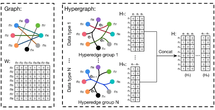
Figure 2: The comparison between graph and hypergraph.

data representation using its flexible hyperedges. For exam-ple, a hypergraph can jointly employ multi-modal data for hypergraph generation by combining the adjacency matrix, as illustrated in Figure 2. Therefore, hypergraph has been employed in many computer vision tasks such as classifi-cation and retrieval tasks (Gao et al. 2012). However, tra-ditional hypergraph learning methods (Zhou, Huang, and Sch¨olkopf 2007) suffer from their high computation com-plexity and storage cost, which limits the wide application of hypergraph learning methods.

In this paper, we propose a hypergraph neural networks framework (HGNN) for data representation learning. In this method, the complex data correlation is formulated in a hy-pergraph structure, and we design a hyperedge convolution operation to better exploit the high-order data correlation for representation learning. More specifically, HGNN is a general framework which can incorporate with multi-modal data and complicated data correlations. Traditional graph convolutional neural networks can be regarded as a special case of HGNN. To evaluate the performance of the pro-posed HGNN framework, we have conducted experiments on citation network classification and visual object recog-nition tasks. The experimental results on four datasets and comparisons with graph convolutional network (GCN) and other traditional methods have shown better performance of HGNN. These results indicate that the proposed HGNN method is more effective on learning data representation us-ing high-order and complex correlations.

The main contributions of this paper are two-fold:

1. We propose a hypergraph neural networks framework, i.e., HGNN, for representation learning using hypergraph structure. HGNN is able to formulate complex and high-order data correlation through its hypergraph structure and can be also efficient using hyperedge convolution operations. It is effective on dealing with multi-modal data/features. Moreover, GCN (Kipf and Welling 2017) can be regarded as a special case of HGNN, for which the edges in simple graph can be regarded as 2-order hy-peredges which connect just two vertices.

2. We have conducted extensive experiments on citation network classification and visual object classification tasks. Comparisons with state-of-the-art methods demon-strate the effectiveness of the proposed HGNN frame-work. Experiments also indicate the better performance of the proposed method when dealing with multi-modal data.

Related Work

In this section, we briefly review existing works of hyper-graph learning and neural networks on hyper-graph.

Hypergraph learning

In many computer vision tasks, the hypergraph structure has been employed to model high-order correlation among data. Hypergraph learning is first introduced in (Zhou, Huang, and Sch¨olkopf 2007), as a propagation process on hypergraph structure. The transductive inference on hypergraph aims to minimize the label difference among vertices with stronger connections on hypergraph. In (Huang, Liu, and Metaxas 2009), hypergraph learning is further employed in video ob-ject segmentation. (Huang et al. 2010) used the hypergraph structure to model image relationship and conducted trans-ductive inference process for image ranking. To further im-prove the hypergraph structure, research attention has been attracted for leaning the weights of hyperedges, which have great influence on modeling the correlation of data. In (Gao et al. 2013), al2regularize on the weights is introduced to learn optimal hyperedge weights. In (Hwang et al. 2008), the correlation among hyperedges is further explored by a assumption that highly correlated hyperedges should have similar weights. Regarding the multi-modal data, in (Gao et al. 2012), multi-hypergraph structure is introduced to assign weights for different sub-hypergraphs, which corresponds to different modalities.

Neural networks on graph

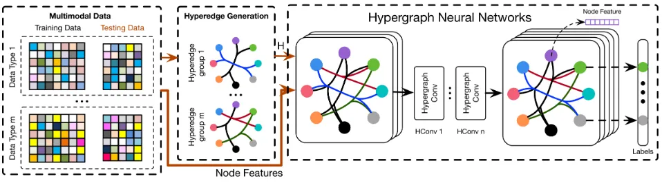
Figure 3: The proposed HGNN framework.

neural networks to graph structure has attracted great atten-tion from researchers. In (Gori, Monfardini, and Scarselli 2005) and (Scarselli et al. 2009), the neural network on graph is first introduced to apply recurrent neural networks to deal with graphs. For generalizing convolution network to graph, the methods are divided into spectral and non-spectral approaches.

For spectral approaches, the convolution operation is for-mulated in spectral domain of graph. (Bruna et al. 2014) in-troduces the first graph CNN, which uses the graph Lapla-cian eigenbasis as an analogy of the Fourier transform. In (Henaff, Bruna, and LeCun 2015), the spectral filters can be parameterized with smooth coefficients to make them spatial-localized. In (Defferrard, Bresson, and Van-dergheynst 2016), a Chebyshev expansion of the graph Laplacian is further used to approximate the spectral filters. Then, in (Kipf and Welling 2017), the chebyshev polynomi-als are simplified into 1-order polynomipolynomi-als to form an effi-cient layer-wise propagation model.

For spatial approaches, the convolution operation is de-fined in groups of spatial close nodes. In (Atwood and Towsley 2016), the powers of a transition matrix is em-ployed to define the neighborhood of nodes. (Monti et al. 2017) uses the local path operators in the form of Gaussian mixture models to generalize convolution in spatial domain. In (Velickovic et al. 2018), the attention mechanisms is in-troduced into the graph to build attention-based architecture to perform the node classification task on graph.

Hypergraph Neural Networks

In this section, we introduce our proposed hypergraph neu-ral networks (HGNN). We first briefly introduce hypergraph learning, and then the spectral convolution on hypergraph is provided. Following, we analyze the relations between HGNN and existing methods. In the last part of the section, some implementation details will be given.

Hypergraph learning statement

We first review the hypergraph analysis theory. Different from simple graph, a hyperedge in a hypergraph connects two or more vertices. A hypergraph is defined as G = (V,E,W), which includes a vertex setV, a hyperedge setE. Each hyperedge is assigned with a weight byW, a diagonal

matrix of edge weights. The hypergraphG can be denoted by a|V| × |E|incidence matrixH, with entries defined as

h(v, e) =

1, ifv∈e

0, ifv6∈e, (1)

For a vertex v ∈ V, its degree is defined as d(v) =

P

e∈Eω(e)h(v, e). For an edgee∈ E, its degree is defined

asδ(e) =P

v∈Vh(v, e). Further,DeandDvdenote the

di-agonal matrices of the edge degrees and the vertex degrees, respectively.

Here let us consider the node(vertex) classification prob-lem on hypergraph, where the node labels should be smooth on the hypergraph structure. The task can be formulated as a regularization framework as introduced by (Zhou, Huang, and Sch¨olkopf 2007):

argmin

f {Remp(f) + Ω(f)}, (2)

whereΩ(f)is a regularize on hypergraph,Remp(f)denotes

the supervised empirical loss,f(·)is a classification func-tion. The regularizeΩ(f)is defined as:

Ω(f) =1 2

X

e∈E

X

{u,v}∈V

w(e)h(u, e)h(v, e)

δ(e)

f(u) p

d(u)−

f(v)

p

d(v)

2

,

(3)

We letθ=D−v1/2HWD−e1H>D −1/2

v and∆=I−Θ.

Then, the normalizedΩ(f)can be written as

Ω(f) =f>∆, (4)

where∆is positive semi-definite, and usually called the hy-pergraph Laplacian.

Spectral convolution on hypergraph

Given a hypergraph G = (V,E,∆) with n vertices, since the hypergraph Laplacian ∆ is a n × n positive semi-definite matrix, the eigen decomposition∆=ΦΛΦ>

can be employed to get the orthonormal eigen vectors

Φ = diag(φ1, . . . , φn) and a diagonal matrix Λ =

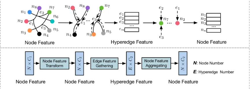
Figure 4: The illustration of the hyperedge convolution layer.

eigenvalues. Then, the Fourier transform for a signalx = (x1, . . . ,xn)in hypergraph is defined asxˆ =Φ>x, where the eigen vectors are regarded as the Fourier bases and the eigenvalues are interpreted as frequencies. The spectral con-volution of signalxand filtergcan be denoted as

g?x=Φ((Φ>g)(Φ>x)) =Φg(Λ)Φ>x, (5) wheredenotes the element-wise Hadamard product and

g(Λ) =diag(g(λ1), . . . ,g(λn))is a function of the Fourier

coefficients. However, the computation cost in forward and inverse Fourier transform is O(n2_{). To solve the} prob-lem, we can follow (Defferrard, Bresson, and Vandergheynst 2016) to parametrizeg(Λ)withK order polynomials. Fur-thermore, we use the truncated Chebyshev expansion as one such polynomial. Chebyshv polynomialsTk(x)is

recur-sively computed byTk(x) = 2xTk−1(x)−Tk−2(x), with T0(x) = 1andT1(x) =x. Thus, theg(Λ)can be parame-tried as

g?x≈

K

X

k=0

θkTk( ˜∆)x, (6)

whereTk( ˜∆)is the Chebyshev polynomial of orderkwith

scaled Laplacian∆˜ = _λ2

max∆−I. In Equation 6, the

ex-pansive computation of Laplacian Eigen vectors is excluded and only matrix powers, additions and multiplications are included, which brings further improvement in computation complexity. We can further let K = 1 to limit the order of convolution operation due to that the Laplacian in hyper-graph can already well represent the high-order correlation between nodes. It is also suggested in (Kipf and Welling 2017) thatλmax ≈ 2 because of the scale adaptability of

neural networks. Then, the convolution operation can be fur-ther simplified to

g?x≈θ0x−θ1D−1/2HWD−e1H>D−v1/2x, (7)

whereθ0 andθ1is parameters of filters over all nodes. We further use a single parameterθto avoid the overfitting prob-lem, which is defined as

_θ

1=−12θ θ0=1₂θD−

1/2

v HD−e1H>D −1/2

v ,

(8)

Then, the convolution operation can be simplified to the following expression

g?x≈ 1

2θD

−1/2

v H(W+I)D−

1

e H>D−

1/2

v x

≈θD−v1/2HWDe−1H>D−v1/2x,

(9)

where(W+I)can be regarded as the weight of the hyper-edges.Wis initialized as an identity matrix, which means equal weights for all hyperedges.

When we have a hypergraph signalX ∈ Rn×C1 _withn

nodes andC1dimensional features, our hyperedge convolu-tion can be formulated by

Y=D−_v1/2HWD_e−1H>D−_v1/2XΘ, (10)

whereW=diag(w1, . . . ,wn).Θ∈RC1×C2_{is the}

param-eter to be learned during the training process. The filterΘ

is applied over the nodes in hypergraph to extract features. After convolution, we can obtainY∈Rn×C2, which can be

used for classification.

Hypergraph neural networks analysis

Figure 3 illustrates the details of the hypergraph neural net-works. Multi-modality datasets are divided into training data and testing data, and each data contains several nodes with features. Then multiple hyperedge structure groups are con-structed from the complex correlation of the multi-modality datasets. We concatenate the hyperedge groups to generate the hypergraph adjacent matrixH. The hypergraph adjacent matrixHand the node feature are fed into the HGNN to get the node output labels. As introduced in the above section, we can build a hyperedge convolutional layerf(X,W,Θ)

in the following formulation

X(l+1)=σ(D_v−1/2HWD−_e1H>D−_v1/2X(l)Θ(l)), (11)

whereX(1) ∈RN×Cis the signal of hypergraph atllayer,

property of exploiting high-order correlation among data. As is shown in Figure 4, the HGNN layer can perform node-edge-node transform, which can better refine the features using the hypergraph structure. More specifically, at first, the initial node featureX(1) _{is processed by learnable} fil-ter matrixΘ(1)_{to extractC}

2-dimensional feature. Then, the node feature is gathered according to the hyperedge to form the hyperedge featureRE×C2_{, which is implemented by the}

multiplication ofH>∈_RE×N_{. Finally the output node}

ture is obtained by aggregating their related hyperedge fea-ture, which is achieved by multiplying matrix H. Denote thatDvandDeplay a role of normalization in Equation 11. Thus, the HGNN layer can efficiently extract the high-order correlation on hypergraph by the node-edge-node transform.

Relations to existing methods When the hyperedges only connect two vertices, the hypergraph is simplified into a sim-ple graph and the Laplacian∆is also coincident with the Laplacian of simple graph up to a factor of 1₂. Compared with the existing graph convolution methods, our HGNN can naturally model high-order relationship among data, which is effectively exploited and encoded in forming feature ex-traction. Compared with the traditional hypergraph method, our model is highly efficient in computation without the in-verse operation of Laplacian∆. It should also be noted that our HGNN has great expansibility toward multi-modal fea-ture with the flexibility of hyperedge generation.

Implementation

Hypergraph construction In our visual object classifica-tion task, the features ofN visual object data can be repre-sented asX= [x1, . . . ,xn]>. We build the hypergraph ac-cording to the distance between two features. More specif-ically, Euclidean distance is used to calculated(xi,xj). In

the construction, each vertex represents one visual object, and each hyperedge is formed by connecting one vertex and its K nearest neighbors, which brings N hyperedges that linksK + 1vertices. And thus, we get the incidence ma-trixH ∈ RN×N withN ×(K+ 1)entries equaling to 1

while others equaling to 0. In the citation network classifi-cation, where the data are organized in graph structure, each hyperedge is built by linking one vertex and their neighbors according to the adjacency relation on graph. So we also get

Nhyperedges andH∈_RN×N_.

Model for node classification In the problem of node classification, we build the HGNN model as in Figure 3. The dataset is divided into training data and test data. Then hypergraph is constructed as the section above, which gen-erates the incidence matrix H and correspondingDe. We build a two-layer HGNN model to employ the powerful ca-pacity of HGNN layer. And the softmax function is used to generate predicted labels. During training, the cross-entropy loss for the training data is back-propagated to update the pa-rametersΘand in testing, the labels of test data is predicted for evaluating the performance. When there are multi-modal information incorporate them by the construction of

hyper-edge groups and then various hyperhyper-edges are fused together to model the complex relationship on data.

Experiments

In this section, we evaluate our proposed hypergraph neu-ral networks on two task: citation network classification and visual object recognition. We also compare the proposed method with graph convolutional networks and other state-of-the-art methods.

Dataset Cora Pumbed

Nodes 2708 19717 Edges 5429 44338 Feature 1433 500 Training node 140 60 Validation node 500 500

Testing node 1000 1000

Classes 7 3

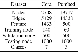
Table 1: Summary of the citation classification datasets.

Citation network classification

Datasets In this experiment, the task is to classify citation data. Here, two widely used citation network datasets, i.e., Cora and Pubmed (Sen et al. 2008) are employed. The ex-perimental setup follows the settings in (Yang, Cohen, and Salakhutdinov 2016). In both of those two datasets, the fea-ture for each data is the bag-of-words representation of doc-uments. The data connection, i.e., the graph structure, in-dicates the citations among those data. To generate the hy-pergraph structure for HGNN, each time one vertex in the graph is selected as the centroid and its connected vertices are used to generate one hyperedge including the centroid itself. Through this we can obtain the same size incidence matrix compared with the original graph. It is noted that as there are no more information for data relationship, the gen-erated hypergraph constructure is quite similar to the graph. The Cora dataset contains 2708 data and 5% are used as la-beled data for training. The Pubmed dataset contains 19717 data, and only 0.3% are used for training. The detailed de-scription for the two datasets listed in Table 1.

Experimental settings In this experiment, a two-layer HGNN is applied. The feature dimension of the hidden layer is set as 16 and the dropout (Srivastava et al. 2014) is em-ployed to avoid overfitting with drop rate p = 0.5. We choose the ReLU as the nonlinear activation function. Dur-ing the trainDur-ing process, we use Adam optimizer (KDur-ingma and Ba 2014) to minimize our cross-entropy loss function with a learning rate of 0.001. We have also compared the proposed HGNN with recent methods in these experiments.

which is 81.6% and 80.1%. As shown in the results, the pro-posed HGNN model can achieve the best or comparable per-formance compared with the state-of-the-art methods. Com-pared with GCN, the proposed HGNN method can achieve a slight improvement on the Cora dataset and 1.1% improve-ment on the Pubmed dataset. We note that the generated hy-pergraph structure is quite similar to the graph structure as there is neither extra nor more complex information in these data. Therefore, the gain obtained by HGNN is not very sig-nificant.

Method Cora Pubmed

DeepWalk (Perozzi, Al-Rfou, and Skiena 2014)

67.2% 65.3%

ICA (Lu and Getoor 2003) 75.1% 73.9% Planetoid (Yang, Cohen, and

Salakhutdinov 2016)

75.7% 77.2%

Chebyshev (Defferrard, Bres-son, and Vandergheynst 2016)

81.2% 74.4%

GCN (Kipf and Welling 2017) 81.5% 79.0%

HGNN 81.6% 80.1%

Table 2: Classification results on the Cora and Pubmed datasets.

Visual object classification

Datasets and experimental settings In this experiment, the task is to classify visual objects. Two public benchmarks are employed here, including the Princeton ModelNet40 dataset (Wu et al. 2015) and the National Taiwan University (NTU) 3D model dataset (Chen et al. 2003), as shown in Ta-ble 3. The ModelNet40 dataset consists of 12,311 objects from 40 popular categories, and the same training/testing split is applied as introduced in (Wu et al. 2015), where 9,843 objects are used for training and 2,468 objects are used for testing. The NTU dataset is composed of 2,012 3D shapes from 67 categories, including car, chair, chess, chip, clock, cup, door, frame, pen, plant leaf and so on. In the NTU dataset, 80% data are used for training and the other 20% data are used for testing. In this experiment, each 3D object is represented by the extracted features. Here, two recent state-of-the-art shape representation methods are employed, including Multi-view Convolutional Neural Net-work (MVCNN) (Su et al. 2015) and Group-View Convolu-tional Neural Network (GVCNN) (Feng et al. 2018). These two methods are selected due to that they have shown sat-isfactory performance on 3D object representation. We fol-low the experimental settings of MVCNN and GVCNN to generate multiple views of each 3D object. Here, 12 virtual cameras are employed to capture views with a interval angle of 30 degree, and then both the MVCNN and the GVCNN features are extracted accordingly.

To compare with GCN method, it is noted that there is no available graph structure in the ModelNet40 dataset and the NTU dataset. Therefore, we construct a probability graph based on the distance of nodes. Given the features of data,

the affinity matrixAis generated to represent the relation-ship among different vertices, andAijcan be calculated by:

Aij = exp(−

2Dij2

∆ ) (12)

whereDij indicates the Euclidean distance between node

i and node j.∆ is the average pairwise distance between nodes. For the GCN experiment with two features con-structed simple graphs, we simply average the two modal-ity adjacency matrices to get the fused graph structure for comparison.

Dataset ModelNet40 NTU

Objects 12311 2012 MVCNN Feature 4096 4096 GVCNN Feature 2048 2048 Training node 9843 1639 Testing node 2468 373

Classes 40 67

Table 3: The detailed information of the ModelNet40 and the NTU datasets.

Figure 5: An example of hyperedge generation in the vi-sual object classification task. Left: For each node we ag-gregate itsN neighbor nodes by Euclidean distance to gen-erate a hyperedge. Right: To gengen-erate the multi-modality hy-pergraph adjacent matrix we concatenate adjacent matrix of two modality.

Hypergraph structure construction on visual datasets

In experiments on ModelNet40 and NTU datasets, two hy-pergraph construction methods are employed. The first one is based on single modality feature and the other one is based on multi-modality feature. In the first case, only one feature is used. Each time one object in the dataset is selected as the centroid, and its 10 nearest neighbors in the selected feature space are used to generate one hyperedge including the cen-troid itself, as shown in Figure 5. Then, a hypergraphGwith

N hyperedges can be constructed. In the second case, mul-tiple features are used to generate a hypergraphGmodeling complex multi-modality correlation. Here, for theith

modal-ity data, a hypergraph adjacent matrixHiis constructed

ac-cordingly. After all the hypergraphs from different features have been generated, these adjacent matricesHican be

Feature

Features for Structure

GVCNN MVCNN GVCNN+MVCNN

GCN HGNN GCN HGNN GCN HGNN

GVCNN (Feng et al. 2018) 91.8% 92.6% 91.5% 91.8% 92.8% 96.6%

MVCNN (Su et al. 2015) 92.5% 92.9% 86.7% 91.0% 92.3% 96.6%

GVCNN+MVCNN - - - - 94.4% 96.7%

Table 4: Comparison between GCN and HGNN on the ModelNet40 dataset.

Feature

Features for Structure

GVCNN MVCNN GVCNN+MVCNN

GCN HGNN GCN HGNN GCN HGNN

GVCNN ((Feng et al. 2018)) 78.8% 82.5% 78.8% 79.1% 75.9% 84.2%

MVCNN ((Su et al. 2015)) 74.0% 77.2% 71.3% 75.6% 73.2% 83.6%

GVCNN+MVCNN − − − − 76.1% 84.2%

Table 5: Comparison between GCN and HGNN on the NTU dataset.

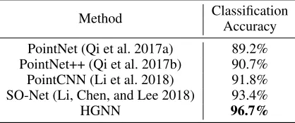
Method Classification Accuracy

PointNet (Qi et al. 2017a) 89.2% PointNet++ (Qi et al. 2017b) 90.7% PointCNN (Li et al. 2018) 91.8% SO-Net (Li, Chen, and Lee 2018) 93.4%

HGNN 96.7%

Table 6: Experimental comparison among recent classifica-tion methods on ModelNet40 dataset.

Results and discussions Experiments and comparisons on the visual object recognition task are shown in Table 4 and Table 5, respectively. For the ModelNet40 dataset, we have compared the proposed method using two features with recent state-of-the-are methods in Table 6. As shown in the results, we can have the following observations:

1. The proposed HGNN method outperforms the state-of-the-art object recognition methods in the ModelNet40 dataset. More specifically, compared with PointCNN and SO-Net, the proposed HGNN method can achieve gains of 4.8% and 3.2%, respectively. These results demon-strate the superior performance of the proposed HGNN method on visual object recognition.

2. Compared with GCN, the proposed method achieves bet-ter performance in all experiments. As shown in Ta-ble 4 and TaTa-ble 5, when only one feature is used for graph/hypergraph structure generation, HGNN can ob-tain slightly improvement. For example, when GVCNN is used as the object feature and MVCNN is used for graph/hypergraph structure generation, HGNN achieves gains of 0.3% and 2.0% compared with GCN on the ModelNet40 and the NTU datasets, respectively. When more features, i.e., both GVCNN and MVCNN, are used for graph/hypergraph structure generation, HGNN achieves much better performance compared with GCN.

For example, HGNN achieves gains of 8.3%, 10.4% and 8.1% compared with GCN when GVCNN, MVCNN and GVCNN+MVCNN are used as the object features on the NTU dataset, respectively.

The better performance can be dedicated to the employed hypergraph structure. The hypergraph structure is able to convey complex and high-order correlations among data, which can better represent the underneath data relation-ship compared with graph structure or the methods without graph structure. Moreover, when multi-modal data/features are available, HGNN has the advantage of combining such multi-modal information in the same structure by its flexible hyperedges. Compared with traditional hypergraph learning methods, which may suffer from the high computational complexity and storage cost, the proposed HGNN frame-work is much more efficient through the hyperedge convo-lution operation.

Conclusion

Acknowledgements

This work was supported by National Key R&D Pro-gram of China (Grant No. 2017YFC0113000, and No.2016YFB1001503), and National Natural Science Funds of China (No.U1705262, No.61772443, No.61572410, No.61671267), National Science and Technology Major Project (No. 2016ZX01038101), MIIT IT funds (Research and application of TCN key technologies) of China, and The National Key Technology R and D Program (No. 2015BAG14B01-02), Post Doctoral Innovative Talent Support Program under Grant BX201600094, China Post-Doctoral Science Foundation under Grant 2017M612134, Scientific Research Project of National Language Commit-tee of China (Grant No. YB135-49), and Nature Science Foundation of Fujian Province, China (No. 2017J01125 and No. 2018J01106).

References

Atwood, J., and Towsley, D. 2016. Diffusion-Convolutional Neural Networks. InNIPS, 1993–2001.

Bruna, J.; Zaremba, W.; Szlam, A.; and LeCun, Y. 2014. Spectral Networks and Locally Connected Networks on Graphs. InProc. ICLR.

Chen, D.-Y.; Tian, X.-P.; Shen, Y.-T.; and Ouhyoung, M. 2003. On Visual Similarity Based 3D Model Retrieval. In

Computer Graphics Forum, volume 22, 223–232. Wiley On-line Library.

Defferrard, M.; Bresson, X.; and Vandergheynst, P. 2016. Convolutional Neural Networks on Graphs with Gast Local-ized Spectral Filtering. InNIPS, 3844–3852.

Feng, Y.; Zhang, Z.; Zhao, X.; Ji, R.; and Gao, Y. 2018. Gvcnn: Group-View Convolutional Neural Networks for 3D Shape Recognition. InProc. CVPR, 264–272.

Gao, Y.; Wang, M.; Tao, D.; Ji, R.; and Dai, Q. 2012. 3-D Object Retrieval and Recognition with Hypergraph Analy-sis. IEEE Transactions on Image Processing 21(9):4290– 4303.

Gao, Y.; Wang, M.; Zha, Z.-J.; Shen, J.; Li, X.; and Wu, X. 2013. Visual-Textual Joint Relevance Learning for Tag-based Social Image Search. IEEE Transactions on Image Processing22(1):363–376.

Gori, M.; Monfardini, G.; and Scarselli, F. 2005. A New Model for Learning in Graph Domains. In Proc. IJCNN, volume 2, 729–734. IEEE.

Henaff, M.; Bruna, J.; and LeCun, Y. 2015. Deep Convolu-tional Networks on Graph-Structured Data. arXiv preprint arXiv:1506.05163.

Huang, Y.; Liu, Q.; Zhang, S.; and Metaxas, D. N. 2010. Image Retrieval via Probabilistic Hypergraph Ranking. In

Proc. CVPR, 3376–3383. IEEE.

Huang, Y.; Liu, Q.; and Metaxas, D. 2009. ] Video Object Segmentation by Hypergraph Cut. InProc. CVPR, 1738– 1745. IEEE.

Hwang, T.; Tian, Z.; Kuangy, R.; and Kocher, J.-P. 2008. Learning on Weighted Hypergraphs to Integrate Protein

In-teractions and Gene Expressions for Cancer Outcome Pre-diction. InProc. ICDM, 293–302. IEEE.

Kingma, D. P., and Ba, J. 2014. Adam: A Method for Stochastic Optimization. InProc. ICLR.

Kipf, T. N., and Welling, M. 2017. Semi-Supervised Classi-fication with Graph Convolutional Networks. InProc. ICLR. Li, Y.; Bu, R.; Sun, M.; and Chen, B. 2018. PointCNN. In

NIPS.

Li, J.; Chen, B. M.; and Lee, G. H. 2018. SO-Net: Self-Organizing Network for Point Cloud Analysis. In Proc. CVPR, 9397–9406.

Lu, Q., and Getoor, L. 2003. Link-based Classification. In

Proc. ICML, 496–503.

Monti, F.; Boscaini, D.; Masci, J.; Rodola, E.; Svoboda, J.; and Bronstein, M. M. 2017. Geometric Deep Learning on Graphs and Manifolds Using Mixture Model CNNs. In

Proc. CVPR, volume 1, 3.

Perozzi, B.; Al-Rfou, R.; and Skiena, S. 2014. Deep-walk: Online Learning of Social Representations. InProc. SIGKDD, 701–710. ACM.

Qi, C. R.; Su, H.; Mo, K.; and Guibas, L. J. 2017a. Point-Net: Deep Learning on Point Sets for 3D Classification and Segmentation.Proc. CVPR1(2):4.

Qi, C. R.; Yi, L.; Su, H.; and Guibas, L. J. 2017b. Point-Net++: Deep Hierarchical Feature Learning on Point Sets in a Metric Space. InNIPS, 5105–5114.

Scarselli, F.; Gori, M.; Tsoi, A. C.; Hagenbuchner, M.; and Monfardini, G. 2009. The Graph Neural Network Model.

IEEE Transactions on Neural Networks20(1):61–80. Sen, P.; Namata, G.; Bilgic, M.; Getoor, L.; Galligher, B.; and Eliassi-Rad, T. 2008. Collective Classification in Net-work Data. AI magazine29(3):93.

Srivastava, N.; Hinton, G.; Krizhevsky, A.; Sutskever, I.; and Salakhutdinov, R. 2014. Dropout: A Simple Way to Prevent Neural Networks from Overfitting. The Journal of Machine Learning Research15(1):1929–1958.

Su, H.; Maji, S.; Kalogerakis, E.; and Learned-Miller, E. 2015. Multi-View Convolutional Neural Networks for 3D Shape Recognition. InProc. ICCV, 945–953.

Velickovic, P.; Cucurull, G.; Casanova, A.; Romero, A.; Lio, P.; and Bengio, Y. 2018. Graph Attention networks. InProc. ICLR, volume 1.

Wu, Z.; Song, S.; Khosla, A.; Yu, F.; Zhang, L.; Tang, X.; and Xiao, J. 2015. 3D ShapeNets: A Deep Representation for Volumetric Shapes. InProc. CVPR, 1912–1920. Yang, Z.; Cohen, W. W.; and Salakhutdinov, R. 2016. Re-visiting Semi-Supervised Learning with Graph Embeddings.

Proc. ICML.

Zhou, D.; Huang, J.; and Sch¨olkopf, B. 2007. Learning with Hypergraphs: Clustering, Classification, and Embedding. In