The Thirty-Third AAAI Conference on Artificial Intelligence (AAAI-19)
A Robust and Efficient Algorithm for the PnL Problem
Using Algebraic Distance to Approximate the Reprojection Distance
Lipu Zhou, Yi Yang, Montiel Abello, Michael Kaess
Robotics Institute, Carnegie Mellon University, Pittsburgh, PA 15213, USA{lipuz,yiy4,mabello,kaess}@andrew.cmu.edu
Abstract
This paper proposes a novel algorithm to solve the pose es-timation problem from 2D/3D line correspondences, known as the Perspective-n-Line (PnL) problem. It is widely known that minimizing the geometric distance generally results in more accurate results than minimizing an algebraic distance. However, the rational form of the reprojection distance of the line yields a complicated cost function, which makes solving the first-order optimality conditions infeasible. Furthermore, iterative algorithms based on the reprojection distance are time-consuming for a large-scale problem. In contrast to pre-vious works which minimize a cost function based on an alge-braic distance that may not approximate the reprojection dis-tance of the line, we design two simple algebraic disdis-tances to gradually approximate the reprojection distance. This speeds up the computation, and maintains the robustness of the ge-ometric distance. The two algebraic distances result in two polynomial cost functions, which can be efficiently solved. We directly solve the first-order optimality conditions of the first problem with a novel hidden variable method. This al-gorithm makes use of the specific structure of the resulting polynomial system, therefore it is more stable than the gen-eral Gr¨obner basis polynomial solver. Then, we minimize the second polynomial cost function by the damped Newton it-eration, starting from the solution of the first cost function. Experimental results show that the first step of our algorithm is already superior to the state-of-the-art algorithms in terms of accuracy and applicability, and faster than the algorithms based on Gr¨obner basis polynomial solver. The second step yields comparable results to the results from minimizing the reprojection distance, but is much more efficient. For speed, our algorithm is applicable to real-time applications.
Introduction
The Perspective-n-Line (PnL) problem is to calculate the rotation and the translation of a camera from N 2D/3D line correspondences. It has broad applications in robotics and 3D vision, such as Structure from Motion (SfM) (Mi-cusik and Wildenauer 2017), and Simultaneous Localization and Mapping (SLAM) (Zhang and Koch 2014), and Aug-mented Reality (AR) (Zhou, Duh, and Billinghurst 2008). Because of its importance, plenty of algorithms have been proposed to address this problem in the literature. However,
Copyright c2019, Association for the Advancement of Artificial Intelligence (www.aaai.org). All rights reserved.
recent work (Pˇribyl, Zemˇc´ık, and ˇCad´ık 2017) has shown that none of the existing methods universally outperforms the others. Algorithms based on Direct Linear Transforma-tion (DLT) (Pˇribyl, Zemˇc´ık, and ˇCad´ık 2017) are fast, but are not stable or even not feasible when the number of linesNis small. Nonlinearly formulated algorithms may be-come very computationally demanding whenN gets large, such as(Mirzaei and Roumeliotis 2011b; Xu et al. 2017; Ansar and Daniilidis 2003). In addition, many PnL algo-rithms are not applicable to the planar configuration (i.e.
all the 3D lines are located on a plane). This paper aims to achieve globally optimal solution for any number and con-figuration of lines with real-time speed.
Minimizing a geometric distance is known to lead to more accurate results than an algebraic distance (Hartley and Zis-serman 2003). However, the reprojection distance of the PnL problem,i.e.the distance between the projection of a 3D line and the end points of the corresponding 2D line in the im-age, results in a non-convex rational cost function. Thus, it is intractable to directly solve its first-order optimality con-ditions. Additionally, the iterative algorithm requires high quality initialization to converge to the globally minimal so-lution, and will become time-consuming when the number of lines grows large. Therefore, different algebraic distances are proposed in the literature to simplify the computation. For example, Xuet al.(Xu et al. 2017) used the residual of the equation from a minimal solution as the cost function. But those algebraic distances may not approximate the re-projection distance. This may lead to a suboptimal solution. The central idea of this paper is to approximate the repro-jection distance with simpler functions. We design two alge-braic distances to achieve this goal.
and Zelevinsky 2008). This method improves the stability of the polynomial solver by taking advantage of the special structure of the resulting polynomial system. It does not clude numerically unstable functions, such as the matrix in-verse involved in the Gr¨obner basis method.
The second algebraic distance formulation involves fix-ing the denominator of the reprojection distance, which re-sults in a polynomial cost function.The reprojection distance is approximated around the point where the denominator is fixed. We apply the damped Newton iteration to minimize the second problem, as it is efficient to calculate the Hessian matrix and gradient of a polynomial function.
The simulation and experimental results show that the first step of our algorithm already outperforms the state-of-the-art methods in terms of accuracy and applicability, and is faster than the algorithms based on Gr¨obner basis poly-nomial solver (Mirzaei and Roumeliotis 2011b; Vakhitov, Funke, and Moreno-Noguer 2016). The result from the sec-ond cost function is comparable to the result from the iter-ative algorithm using the reprojection cost function, but is much faster. Lastly, our algorithm is fast enough for real-time applications.
Related Work
The PnL problem has been widely studied in the literature. At least three 2D/3D line correspondences are required to compute the pose. The minimal problem of PnL is called the P3L problem. Some algorithms have been proposed to address the P3L problem (Dhome et al. 1989; Chen 1990; Xu et al. 2017). They showed that there may exist at most 8 solutions to the P3L problem. Recently, Xuet al.(Xu et al. 2017) systematically analyzed the relationship between the number of solutions and the configuration of the three lines. The P3L algorithm is generally used in the RANSAC framework (Fischler and Bolles 1987) to eliminate outliers.
As mentioned above, the geometric distance of the PnL problem is complicated. Iterative algorithms give a straight forward way to address the minimization problem. In an early work (Liu, Huang, and Faugeras 1990), rotation and translation were calculated separately. They calculated the rotation by iteratively linearizing the equation. In (Kumar and Hanson 1994), the rotation and translation were jointly optimized. Davidet al.(David et al. 2003) simultaneously estimated the pose and the correspondence between 2D and 3D lines in an iterative manner. Recent work (Zhang et al. 2016) presented a noise model to describe the probabilistic relationship between the 3D line and its image. Using this model, they derived a maximum likelihood estimation of the camera pose. Iterative methods may converge to a local min-imum. In addition, iterative algorithms are time-consuming for a large-scale problem.
To reduce the computational complexity, some works seek to linearize the reprojection distance or an algebraic distance. The DLT method (Hartley and Zisserman 2003) gives a fast way to solve the PnL problem. It needs at least 6 lines. Recently, Pˇribyl et al.(Bronislav Pˇribyl 2015) ex-ploit the relationship between the projection of the Pl¨ucker coordinates and the 2D line to construct linear equations. This algorithm needs at least 9 lines. In their later work
(Pˇribyl, Zemˇc´ık, and ˇCad´ık 2017), they combined the tradi-tional DLT method (Hartley and Zisserman 2003) and their Pl¨ucker coordinates based DLT method (Bronislav Pˇribyl 2015) to further improve the accuracy, and reduced the min-imum number of line correspondences to 5. Ansar and Dani-ilidis (Ansar and DaniDani-ilidis 2003) proposed an algorithm to linearize a quadratic equation system to a linear system. The
O n2computational complexity of this algorithm makes it impracticable for a large-scale problem. As these meth-ods ignore the nonlinear part of the constraints, they are not accurate or even feasible whenNis small.
To solve the problem of linearization, nonlinear alge-braic distances are designed to replace the reprojection dis-tance in some recent works. Xu et al. (Xu et al. 2017) used the minimal solution to construct a 16th order polyno-mial cost function. This algorithm is accurate and efficient when N is small, but becomes less accurate and computa-tionally demanding as N grows large as demonstrated in (Pˇribyl, Zemˇc´ık, and ˇCad´ık 2017). Mizaeiet al. (Mirzaei and Roumeliotis 2011a; 2011b) decoupled the estimation of rotation and translation. They directly solve the first-order optimality conditions of the rotation matrix to obtain all stationary points. Some works extended the Perspective-n-Point (PnP) algorithms to the PnL problem. Vakhitovet al. (Vakhitov, Funke, and Moreno-Noguer 2016) and Xu
et al.(Xu et al. 2017) adapted the EPnP algorithm (Lep-etit, Moreno-Noguer, and Fua 2008) to the PnL problem. Vakhitovet al.(Vakhitov, Funke, and Moreno-Noguer 2016) showed that OPnP algorithm (Zheng et al. 2013) can be used to solve the PnL problem. As these algebraic distances do not approximate the geometric distance, this may result in suboptimal results. This paper aims to approximate the re-projection function to efficiently obtain the globally optimal solution.
Problem Formulation
Throughout this paper we use italic, boldfaced lowercase and boldfaced uppercase letters to represent scalars, vec-tors and matrices, respectively. To simplify the notation, we use the normalized pixel coordinates (Hartley and Zisserman 2003),i.e.multiplying the homogeneous pixel coordinates by the inverse of the camera intrinsic parameter matrix K
before solving the PnL problem.
The PnL problem is to estimate the pose of a camera, including rotation R and translationt relative to a world frame, by N(N ≥3) 2D/3D lines correspondences. The minimal case isN = 3, called the P3L problem, which has at most 8 solutions (Xu et al. 2017). ForN ≥4, there gen-erally only exists one solution.
We use the Cayley–Gibbs–Rodriguez (CGR) parametrization (Mirzaei and Roumeliotis 2011b) to representRas
R= R¯
1 +sTs,R¯ = 1−s Ts
I3+ 2[s]×+ 2ss
T
, (1)
wheres= [s1;s2;s3]is a 3-dimensional vector and[s]× =
" 0 −s
3 s2
s3 0 −s1
−s2 s1 0
#
param-eterizations, the CGR parameterization also has a singu-lar case, that is when the rotation angle equals to π. This can be easily solved by rotating the measurements to an intermediate frame, then rotating the solutions back to the original frame, as mentioned by (Mirzaei and Roumelio-tis 2011a). In practice, the RANSAC algorithm is generally used before the least-squares algorithm. The solution from the RANSAC algorithm can be used to rotate the measure to a non-singular case. The advantage of the CGR parameteri-zation is that it does not require additional constraints, such as the unity norm condition of the quaternion parameteriza-tion. This leads to a simple formulaparameteriza-tion.
We adopt the Pl¨ucker coordinates (Pˇribyl, Zemˇc´ık, and ˇ
Cad´ık 2017; Hartley and Zisserman 2003) to represent the 3D line. For theith 3D lineLi, we denote its Pl¨ucker coor-dinates as a six-dimensional vectorLi = [di;mi].di and
mi are the direction vector and moment vector of Li, re-spectively, and they satisfydi·mi = 0, where·represents
the dot product. Letc = −RTt. Denote the projection of
Lito the image plane asli, as demonstrated in Figure 1. The relationship betweenLiandliis:
li∼
R,−R[c]×
Li, (2)
where∼represents the two homogeneous entities are equal up to scale. Letli =l1i, li2, li3
. Assume the ideal 2D line
li corresponding to Li is detected by a line detection al-gorithm, such as (Von Gioi et al. 2010), asˆli. Because of noise, for example motion blur and rounding error, the ideal projectionli and the observationˆli are different. Suppose
ˆ
pij = [ˆxij; ˆyij; 1], j = 1,2 are the homogeneous coordi-nates of the two endpoints ofˆli.pˆij does not generally lie onli. The signed reprojection distance for theith 2D/3D line correspondence is:
erepij =q pˆij·li (l1
i)
2
+ (l2
i)
2 (3)
The cost function based on the reprojection distance is:
Crep= 1 2
X
i X
j
erepij 2
(4)
According to the CGR parameterization ofRin (1), the de-nominator and the numerator of eerpij 2
are both 6th de-gree polynomial functions involvings andc, respectively. As the denominator oferepij is different for each 2D/3D line correspondence, the degrees of the polynomials in the de-nominator and the numerator of the summation Crep will quickly increase as the number of measurements increases. This makes calculating the first-order optimality conditions of (4) intractable. This paper seeks to solve this problem.
Optimal Solution from Algebraic Distance
The central idea of this paper is to approximate the reprojec-tion distanceerepij by simpler functions, whose gradient and Hessian matrix can be easily computed. We use two alge-braic distances to achieve this.Figure 1: Schematic of the reprojection distance.
First Algebraic Distance
AssumePij, j = 1,2are two 3D points onLi. Denote the
homogeneous coordinates of the projection of Pij in the image plane as pij. Using the normalized pixel, we have
pij∼RP j
i+t. Theoretically,pijshould be on the 2D line
ˆli, thus we have
ˆli·(RPij+t) = 0. (5)
In contrast to (3), we can decoupleRandtfrom (5). Astis unconstrained and linear in (5), we first consider the solution oft. GivenR, we derive a linear equation oftfrom (5) as:
ˆli·t=−ˆli·RPij. (6)
This is a linear unconstrained least-squares problem. Solv-ing fort, we obtain a closed-form solution oftas
t=− LTL−1
LTb(R), (7)
where L = hˆl1,ˆl1,· · ·,ˆlN,ˆlN iT
, b(R) =
h
ˆlT
1RP11,ˆlT1RP12,· · ·,lTNRPN1,lTNRPN2
iT
. Sub-stituting the CGR parametrization ofRin (1) into (7), we have
t=− L
TL−1
LTb ¯R
1 +sTs (8)
Then substituting (1) and (8) into (5), we obtain
ˆl
i·RP¯ ij+ˆli· LTL −1
LTb ¯R
1 +sTs = 0. (9) Cancelling the denominator1 +sTsfrom (9), we get a poly-nomial constraint involving onlys:
eaijlg 1 =ˆli·RP¯ ij+ˆli· LTL −1
LTb ¯R
= 0. (10)
Considering the noise, we form the following least-squares problems for (10),
ˆ
s= arg min
s Calg1, Calg1=
1 2
X
i X
j
ealgij 1
2
Asealgij 1is a second-order polynomial function ofs,Calg1is
a fourth-order polynomial function. To find the optimal so-lution ofCalg1, we consider the first-order optimality
condi-tions of it,
f1=
∂Calg1
∂s1
= 0, f2=
∂Calg1
∂s2
= 0, f3=
∂Calg1
∂s3
= 0
(12) This is a ternary polynomial system of degree 3. We do not adopt the generally used Gr¨obner basis method (Zheng et al. 2013; Mirzaei and Roumeliotis 2011a; 2011b) to solve (12), since it may be plagued by numeric problems. Due to the special structure of (12), this equation system can be ef-fectively solved by the hidden variable method according to the theory in Cox, Little, and O’Shea (2006); Gelfand, Kapranov, and Zelevinsky (2008). This method does not volve numerically unstable functions, such as the matrix in-verse used in the Gr¨obner basis method. Therefore, it could be more stable.
Without loss of generality, we treat s1 and s2 as
un-knowns, ands3as a constant. Thus we have
fi=ais31+bis21s2+cis1s22+dis32+pi1(s3)s21+
pi2(s3)s1s2+pi3(s3)s22+pi4(s3)s1+ (13)
pi5(s3)s2+pi6(s3) = 0, i= 1,2,3,
wherepin(s3)(n = 1,· · · ,6) are polynomial functions of
s3. Then we convertfito a homogeneous equation by intro-ducing an auxiliary variables0to make all the monomials in
fi have degree three. This results in the following homoge-neous equation system:
Fi=ais31+bis21s2+cis1s22+dis32+pi1(s3)s0s21+
pi2(s3)s0s1s2+pi3(s3)s0s22+pi4(s3)s20s1+ (14)
pi5(s3)s20s2+pi6(s3)s30= 0, i= 1,2,3.
We can find thatFi=fiwhens0= 1. That is to say, given
s3, if[s1, s2]is a solution of (13),[1, s1, s2]will be a solution
of (14), and vice versa.
Assume thata,bandcare non-negative integers and sat-isfy a+b+c = 2, such asa = 2, b = 0, c = 0. There are clearly 6 choices fora,bandc. Each of them will result in a 4th-order polynomial equation. For each choice, we can writeF1,F2andF3as
F1=sa0+1P1+s1b+1Q1+sc2+1R1,
F2=sa0+1P2+s1b+1Q2+sc2+1R2,
F3=sa0+1P3+s1b+1Q3+sc2+1R3.
(15)
Let us takea= 2, b= 0, c= 0as an example. According to (15), we have
Fi=s30Pi+s1Qi+s2Ri, i= 1,2,3 (16)
where Pi = pi6(s3), Qi = ais21 + bis1s2 + cis22 +
pi1(s3)s0s1 +pi2(s3)s0s2 +pi4(s3)s20, Ri = dis0s22 +
pi3(s3)s0s2+pi5(s3)s20.
The representation ofPi,Qi andRi is not uniform, but the solution of the polynomial system is independent of the choice of them as proved in (Gelfand, Kapranov, and
Zelevinsky 2008). The above equations can be treated as a linear homogeneous system forsa0+1,sb1+1andsc2+1. If the polynomial system F1 = 0, F2 = 0, F3 = 0 has a
non-trivial solution, the determinant of the coefficient matrix in (15) should be zero. Then, we get
Fabc= det
P1 Q1 R1
P2 Q2 R2
P3 Q3 R3
!
= 0, (17)
wheredet (·)represents the determinant of a matrix. We can obtain 6Fabcin (17) for the 6 possible combinations ofa+
b+c= 2. On the other hand, the solutions ofF1= 0, F2=
0, F3= 0are also the solutions of the following equations
uFi= 0, u=s0, s1, s2, i= 1,2,3. (18)
We can have 9uFiin (18).FabcanduFiare all fourth-order polynomials in s0,s1 ands2. Combining these equations,
we have a linear homogeneous system of 15 equations and 15 monomials
M(s3)S=0 (19)
whereM(s3)is a15×15matrix with polynomials ins3as
elements, andS= [s4
0, s30s1, s30s2, s20s21, s20s1s2, s20s22, s0s31,
s0s21s2, s0s1s22, s0s32, s41, s31s2, s21s22, s1s32, s42]T.
The linear homogeneous systemM(s3)S=0has a
non-trivial solution if and only ifdet (M(s3)) = 0. This can be
formulated as a polynomial eigenvalue problem and can be efficiently addressed (Fitzgibbon 2001). After computing
s3, we solve the linear homogeneous equation (19) for S.
The solutions ofs1 ands2 can be found from the second
and third terms inS,i.e.s30s1ands30s2, by settings0= 1as
mentioned above. Then we can getRfrom (1) and tfrom (8). As there are multiple solutions of (12), we choose the one with the smallest cost in (4) as the optimal solution.
Second Algebraic Distance
The global minimizer of the algebraic distance (11) is prob-ably not the optimal solution of (4). The global minimizer of the reprojection distance generally provides better results (Hartley and Zisserman 2003). After obtaining the initial es-timation ofRandt, iterative optimization algorithms on the reprojection error can be used to refine the solution. How-ever, this is time-consuming for a large-scale problem. To solve this problem, we introduce a second algebraic distance that approximates the reprojection distance (3), but its Hes-sian matrix and gradient are easy to calculate.
One problem of erepij in (3) is that its denominator in-volves Randt, and varies for different 2D/3D line corre-spondences. Thus, it is difficult to calculate the cost function in (4). However, if we fix the denominator of (3) at a certain
R0andt0, we can get an approximation of (3) aroundR0
andt0. We define our second algebraic distance as:
ealgij 2=q ˆpij·li (l1
i(R0,t0)) 2
+ (l2
i(R0,t0))
2. (20)
This yields the least-squares problem as:
ˆs,ˆt= arg min
s,t Calg2, Calg2=
1 2
X
i X
j
ealgij 2
2
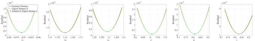
Figure 2: Compare the reprojection distance based cost functionCrepwith our second algebraic distance based cost function
Calg2using 10 lines with zero-mean 2 pixels standard deviation Gaussian Noise. The denominator oferepij is fixed at the solution of the first algebraic distance. We can find thatCrepandCalg2are very similar. Each figure is obtained by varying one variable
and fixing the remaining variables.
WhenR0andt0are close to the optimal solution,ealgij 2 will approximate erepij around the optimal solution. Thus
Calg2will accordingly approximateCreparound the optimal solution. Figure 2 comparesCalg2withCrepfor 10 lines. It is obvious thatCalg2 can well approximateCrepusing the solution from the first step. As the denominator of (20) is a scalar now,ealgij 2 is a polynomial function. We can easily calculate the summationCalg2.
We do not directly solve the first-order optimality con-dition of Calg2. Instead, we use the damped Newton
iter-ation to minimize this function, as the Hessian matrix and the gradient can be efficiently calculated for the polynomial function. The iterative algorithm is initialized with the so-lution from the first step. For thekth iteration, we compute the Hessian matrix H and the gradient vector∇Calg2 of
Calg2. Then we update the solution with [sk+1;tk+1] =
[sk;tk]−(H+λI6)
−1
∇Calg2.λis adjusted according to
the LM algorithm (Mor´e 1978) to ensure the cost function is reduced at every step.
We can repeat this process again when the minimization ofCalg2 converges. But we did not observe significant
im-provement for additional iterations in our experiments. This is because the result from the first step is close to the optimal solution. In this case,Calg2 can well approximateCrep, as illustrated in Figure 2. As a result, the global minimum of
Calg2approximates the global minimum ofCrep.
We summarize the main part of our algorithm as follows: Input:N(N ≥3)2D/3D line correspondences
Output: camera poseRandtrelative to the world frame
1. Construct the cost functionCalg1in (11).
2. Solve the first-order optimality conditions of Calg1
with the hidden variable method introduced above to get the CGR parameterss. Then solve fortby (8). 3. Chooses0andt0with the minimal cost of (4) as the
solution.
4. ConstructCalg2usings0andt0, and minimizeCalg2
by the damped Newton iteration.
Experiments
In this section, we compare our algorithm, referred to as OAPnL, with previous works including OPnPL
(Vakhi-tov, Funke, and Moreno-Noguer 2016), DLTCom-bined Lines(Bronislav Pˇribyl 2015),DLT Plucker Lines (Pˇribyl, Zemˇc´ık, and ˇCad´ık 2017), LPnL DLT (Xu et al. 2017),LPnL Bar LS (Xu et al. 2017),LPnL Bar ENull (Xu et al. 2017), ASPnL (Xu et al. 2017), Ansar(Ansar and Daniilidis 2003), Mirzaei (Mirzaei and Roumeliotis 2011b). We evaluate the results from the two steps of our algorithm denoted as OAPnL I and OAPnL II, respec-tively. We also minimize the reprojection cost (4) by the LM method (Mor´e 1978), initialized by the solution of OAPnL I. We denote it asOAPnL I+GeoLM. We do not consider the 2D/3D endpoint mismatching problem as most related works, since it can be solved by shifting the endpoint and computing a new PnL problem (Vakhitov, Funke, and Moreno-Noguer 2016). Thus we focus on the accuracy of the PnL algorithm itself. The algorithms are evaluated by accuracy and computational time.
Experiments with Synthetic Data
The virtual camera has resolution640×480pixels and fo-cal length 800. The camera is randomly placed within a [−10m,10m]3 cube. We uniformly sample the Euler an-gles α, β, γ of the rotation matrix (α, γ ∈ [0◦,360◦]and
β ∈ [0◦,180◦]).N 2D/3D line correspondences are
ran-domly yielded for each trial using the method in (Xu et al. 2017). Specifically, we first generate the end points of the 2D lines, then the corresponding 3D lines are reconstructed by back-projecting the end points of the 2D lines. The depths of the 3D points are within[4m,10m]. In addition to the configuration that the 2D line segments are uniformly dis-tributed in the whole image (denoted ascentered case), we also considered two challenging configurations mentioned is the literature, i.e.uncentered case(Xu et al. 2017) and planar case(Vakhitov, Funke, and Moreno-Noguer 2016). In theuncentered case, the 2D line segments are within the region[0,160]×[0,120]pixels. In theplanar case, all the 3D lines are on a plane. We randomly generate a plane in front of the camera, then calculate the intersection lines be-tween the back-projections of the 2D lines and the plane.
The result of each experiment is obtained from 500 inde-pendent trials. Denote the estimated rotation and translation asRˆandˆt, and the ground truth asRgtandtgt. We evaluate the rotation error by the angle of the axis-angle representa-tion ofR−gt1Ras Pˇribyl, Zemˇc´ık, and ˇCad´ık (2017), and the translation error bytgt−ˆt
2
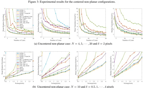
Figure 3: Experimental results for the centered non-planar configurations.
Figure 4: Experimental results for the uncentered non-planar configurations.
Nonplanar case We first consider the non-planar case. We evaluate the robustness of different algorithms by two
num-Figure 5: Experimental results for the centered planar configuration
ber of 2D/3D line correspondencesN from 4 to 20 with a fixed standard deviationδ = 2pixels. The second exper-iment keepsN = 10, whileδ is increased from 0.5 to 4 pixels. The means and medians of the rotation and trans-lation errors are shown in Figure 3 and 4. The uncentered case is more challenging than the centered case. The estima-tion error of each algorithm is larger in the uncentered case. Our algorithm is superior to the previous works. The results fromOAPnL Iare already more accurate than the previous works, and are close to the results fromOAPnL I+GeoLM. OAPnL IIgives better result thanOAPnL I, and is compa-rable withOAPnL I+GeoLM.
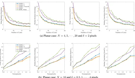
Planar case Most of the algorithms fail to deal with the planar case, including some nonlinear formulation algo-rithms, such as ASPnL (Xu et al. 2017) and Mirzaei (Mirzaei and Roumeliotis 2011b). This phenomenon is also observed in (Pˇribyl, Zemˇc´ık, and ˇCad´ık 2017) and (Vakhitov, Funke, and Moreno-Noguer 2016). As in the non-planar case, we evaluate the robustness of different algorithms by two ex-periments, i.e. varying N ∈ [4,20] while fixing δ = 2 pixels, and increasingδfrom 0.5 to 4 pixels with step 0.5 while keepingN = 10. For the line distribution, we consider the centered case. We compared our algorithm withOPnPL andEPnPL Planar.EPnPL Planaris an extension of the planarEPnPalgorithm (Lepetit, Moreno-Noguer, and Fua 2008) to the PnL problem introduced in Vakhitov, Funke, and Moreno-Noguer (2016). Figure 5 shows the results of different algorithms. It is clear that our algorithm outper-forms other algorithms. In most cases, OAPnL II gives comparable result to OAPnL I+GeoLM. When the noise is large as shown in Figure 5 (b),OAPnL I+GeoLMgives
slightly better result thanOAPnL II. This is because the so-lution ofOAPnL Imay diverge away from the optimal so-lution when the noise increases. This enlarges the difference betweenealgij 2anderepij around the optimal solution.
Experiments with Real Data
We also compare our algorithm with previous works using real images. Ten datasets (including VGG dataset and MPI dataset (Jain et al. 2010) ) with ground truth camera poses and 2D/3D line correspondences are used to evaluate the al-gorithms. The details of the datasets are listed in Table 1.
In this experiment, we use the absolute translation error
tgt−ˆt
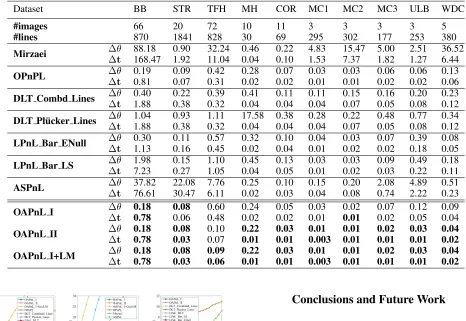
2as (Pˇribyl, Zemˇc´ık, and ˇCad´ık 2017). The rota-tion error is the same as the experiment with synthetic data. We compute the mean rotation and translation errors of our algorithm and OPnPL. The estimation errors of other al-gorithms are from Pˇribyl, Zemˇc´ık, and ˇCad´ık (2017). The experimental results are shown in Table 1. Our algorithm OAPnL I and OAPnL II outperform other algorithms. OAPnL IIgives similar results asOAPnL I+GeoLM.
Computational Time
We evaluate the computational time of different algorithms on a laptop with a i7 2.9 GHZ cpu. The number of lines
Table 1: Experimental results and dataset characteristics.∆θ(◦)is the angle of the angle-axis representation ofRgt−1Rˆ.∆t(m) is the absolute translation errortgt−ˆt
2. The best results are labeled by bold font.
Dataset BB STR TFH MH COR MC1 MC2 MC3 ULB WDC
#images 66 20 72 10 11 3 3 3 3 5
#lines 870 1841 828 30 69 295 302 177 253 380
Mirzaei ∆θ 88.18 0.90 32.24 0.46 0.22 4.83 15.47 5.00 2.51 36.52 ∆t 168.47 1.92 11.04 0.04 0.10 1.53 7.37 1.82 1.27 6.44
OPnPL ∆θ 0.19 0.09 0.42 0.28 0.07 0.03 0.03 0.06 0.06 0.13 ∆t 0.81 0.07 0.31 0.02 0.02 0.01 0.01 0.02 0.02 0.06
DLT Combd Lines ∆θ 0.40 0.22 0.39 0.41 0.11 0.11 0.15 0.16 0.20 0.23 ∆t 1.88 0.38 0.32 0.04 0.04 0.04 0.07 0.05 0.08 0.12
DLT Pl ¨ucker Lines ∆θ 1.04 0.93 1.11 17.58 0.38 0.28 0.22 0.48 0.77 0.34 ∆t 1.88 0.38 0.32 0.04 0.04 0.04 0.07 0.05 0.08 0.12
LPnL Bar ENull ∆θ 0.30 0.11 0.57 0.32 0.10 0.04 0.03 0.07 0.39 0.08 ∆t 1.13 0.16 0.45 0.02 0.04 0.01 0.02 0.02 0.18 0.05
LPnL Bar LS ∆θ 1.98 0.15 1.10 0.45 0.13 0.03 0.03 0.09 0.49 0.18 ∆t 7.23 0.27 1.05 0.04 0.05 0.01 0.02 0.03 0.22 0.11
ASPnL ∆θ 37.82 22.08 7.76 0.25 0.10 0.15 0.20 2.08 4.89 0.51 ∆t 76.61 30.47 6.11 0.02 0.03 0.04 0.08 0.74 2.22 0.23
OAPnL I ∆θ 0.18 0.08 0.60 0.24 0.05 0.03 0.02 0.07 0.12 0.09 ∆t 0.78 0.06 0.48 0.02 0.02 0.01 0.01 0.02 0.05 0.04
OAPnL II ∆θ 0.18 0.08 0.10 0.22 0.03 0.01 0.01 0.02 0.03 0.04 ∆t 0.78 0.03 0.07 0.01 0.01 0.003 0.01 0.01 0.01 0.02 OAPnL I+LM ∆θ 0.18 0.08 0.09 0.22 0.03 0.01 0.01 0.02 0.03 0.04 ∆t 0.78 0.03 0.06 0.01 0.01 0.003 0.01 0.01 0.01 0.02
Figure 6: (a) Computation time of all the algorithms. (b) Computational time of algorithms based on nonlinear for-mulation. (c) Computation time of our algorithm and algo-rithms based on linear formulation
LPnL DLTwhenNis large. However, our algorithm is su-perior to them in terms of accuracy and applicability. Fig-ure 6 (b) illustrates the computational time of the algorithms based on nonlinear formulation.OAPnL Iis faster than all of them exceptASPnLwhenN is small, asASPnLonly needs to solve a 15th order polynomial equation. But the running time ofASPnLquickly increases, thus it is not suit-able for real-time applications whenN is large.OAPnL II is much more efficient thanOAPnL I+GeoLM.OAPnL I and OAPnL II can process 1000 lines around 5ms and 11ms, respectively. Thus, our algorithm is applicable to real-time applications.
Conclusions and Future Work
In this paper we propose a novel algorithm to address the PnL problem. We design two algebraic distances to approx-imate the reprojection distance. The PnL problem is solved by consecutively minimizing two polynomial cost functions derived from the two algebraic distances. We introduce a novel hidden variable method to solve the first-order opti-mality conditions of the first problem. This method utilizes the special structure of the resulting polynomial system. This makes it more stable than the general Gr¨obner basis based methods adopted in the previous works. This method can be extended to other problems which are formulated as a similar polynomial system. We adopt the damped Newton iteration to minimize the second minimization problem, as the Hessian matrix and the gradient can be efficiently cal-culated for the polynomial cost function. We evaluated our algorithm by experiments on synthetic and real data. The results show that the first algebraic distance alone outper-forms the state-of-the-art methods in terms of accuracy and applicability. The second step is comparable to the iterative method based on the reprojection distance, but much faster. Our proposed algorithm is scalable and applicable to real-time applications.
A more efficient method to solve (19) is to compute det (M(s3)) by the quotient-free Gaussian Elimination
References
Ansar, A., and Daniilidis, K. 2003. Linear pose estimation from points or lines.IEEE Transactions on Pattern Analysis and Machine Intelligence25(5):578–589.
Bronislav Pˇribyl, Pavel Zemˇc´ık, M. ˇC. 2015. Camera pose estimation from lines using pl¨ucker coordinates. In Pro-ceedings of the British Machine Vision Conference (BMVC 2015), 1–12. The British Machine Vision Association and Society for Pattern Recognition.
Byr¨od, M.; Josephson, K.; and ˚Astr¨om, K. 2009. Fast and stable polynomial equation solving and its application to computer vision. International Journal of Computer Vision
84(3):237–256.
Chen, H. H. 1990. Pose determination from line-to-plane correspondences: Existence condition and closed-form so-lutions. InProceedings Third International Conference on Computer Vision, 374–378. IEEE.
Cox, D. A.; Little, J.; and O’shea, D. 2006.Using algebraic geometry, volume 185. Springer Science & Business Media. David, P.; DeMenthon, D.; Duraiswami, R.; and Samet, H. 2003. Simultaneous pose and correspondence determina-tion using line features. InProceedings of IEEE Computer Society Conference on Computer Vision and Pattern Recog-nition, volume 2, II–424–II–431 vol.2.
Dhome, M.; Richetin, M.; Lapreste, J. T.; and Rives, G. 1989. Determination of the attitude of 3d objects from a sin-gle perspective view.IEEE Transactions on Pattern Analysis and Machine Intelligence11(12):1265–1278.
Fischler, M. A., and Bolles, R. C. 1987. Random sample consensus: a paradigm for model fitting with applications to image analysis and automated cartography. InReadings in computer vision. Elsevier. 726–740.
Fitzgibbon, A. W. 2001. Simultaneous linear estimation of multiple view geometry and lens distortion. In Proceed-ings of the 2001 IEEE Computer Society Conference on Computer Vision and Pattern Recognition. CVPR 2001, vol-ume 1, 125–132.
Gelfand, I. M.; Kapranov, M.; and Zelevinsky, A. 2008. Dis-criminants, resultants, and multidimensional determinants. Springer Science & Business Media.
Hartley, R., and Li, H. 2012. An efficient hidden variable approach to minimal-case camera motion estimation. IEEE Transactions on Pattern Analysis and Machine Intelligence
34(12):2303–2314.
Hartley, R., and Zisserman, A. 2003.Multiple view geometry in computer vision. Cambridge university press.
Jain, A.; Kurz, C.; Thorm¨ahlen, T.; and Seidel, H.-P. 2010. Exploiting global connectivity constraints for reconstruction of 3d line segment from images. InIEEE Conference on Computer Vision and Pattern Recognition (CVPR 2010). Kumar, R., and Hanson, A. 1994. Robust methods for esti-mating pose and a sensitivity analysis. CVGIP: Image Un-derstanding60(3):313 – 342.
Lepetit, V.; Moreno-Noguer, F.; and Fua, P. 2008. Epnp: An accurate o(n) solution to the pnp problem. International Journal of Computer Vision81(2):155.
Liu, Y.; Huang, T. S.; and Faugeras, O. D. 1990. Determi-nation of camera location from 2-d to 3-d line and point cor-respondences. IEEE Transactions on pattern analysis and machine intelligence12(1):28–37.
Micusik, B., and Wildenauer, H. 2017. Structure from mo-tion with line segments under relaxed endpoint constraints.
International Journal of Computer Vision124(1):65–79. Mirzaei, F. M., and Roumeliotis, S. I. 2011a. Globally opti-mal pose estimation from line correspondences. In Proceed-ings of 2011 IEEE International Conference on Robotics and Automation, 5581–5588.
Mirzaei, F. M., and Roumeliotis, S. I. 2011b. Optimal es-timation of vanishing points in a manhattan world. In Pro-ceedings of 2011 International Conference on Computer Vi-sion, 2454–2461.
Mor´e, J. J. 1978. The levenberg-marquardt algorithm: im-plementation and theory. InNumerical analysis. Springer. 105–116.
Pˇribyl, B.; Zemˇc´ık, P.; and ˇCad´ık, M. 2017. Absolute pose estimation from line correspondences using direct lin-ear transformation. Computer Vision and Image Under-standing161:130 – 144.
Pˇribyl, B.; Zemˇc´ık, P.; and ˇCad´ık, M. 2017. Absolute pose estimation from line correspondences using direct lin-ear transformation. Computer Vision and Image Under-standing.
Vakhitov, A.; Funke, J.; and Moreno-Noguer, F. 2016. Accu-rate and linear time pose estimation from points and lines. In Leibe, B.; Matas, J.; Sebe, N.; and Welling, M., eds., Com-puter Vision – ECCV 2016, 583–599. Cham: Springer Inter-national Publishing.
Von Gioi, R. G.; Jakubowicz, J.; Morel, J.-M.; and Randall, G. 2010. Lsd: A fast line segment detector with a false detection control.IEEE transactions on pattern analysis and machine intelligence32(4):722–732.
Xu, C.; Zhang, L.; Cheng, L.; and Koch, R. 2017. Pose esti-mation from line correspondences: A complete analysis and a series of solutions.IEEE Transactions on Pattern Analysis and Machine Intelligence39(6):1209–1222.
Zhang, L., and Koch, R. 2014. Structure and motion from line correspondences: Representation, projection, initializa-tion and sparse bundle adjustment. Journal of Visual Com-munication and Image Representation25(5):904 – 915. Zhang, Y.; Li, X.; Liu, H.; and Shang, Y. 2016. Probabilistic approach for maximum likelihood estimation of pose using lines. IET Computer Vision10(6):475–482.