An open geographic modeling environment.

TECHNICAL ARTICLE

An

_Open

_Geographic

Modeling

Environment

Thomas Maxwell Robert Costanza

University

of Maryland

Institute for

_Ecological

Economics

Solomons,

MD maxwell @ kabir.cbl.cees.edu

[email protected]

Developing

the

_complex

_computer

models that are _necessary

_{for effectively managing}

human

_{affairs through}

the next

_century

requires

new

_{infrastructure supporting high}

performance

collaborative

_modeling.

In this paper we describe our

_Open

_Geographic

Modeling

Environment,

which

_supports:

₍₁₎

modular,

hierarchical model construction and

_{archiving/linking of}

simulation

modules,

_{(2) graphical,}

icon-based model

construction,

(3)

transparent

distributed

computing,

and

₍₄₎

_{integrating multiple}

space-time representations.

This

environment,

which

_{transparently}

links icon-based

_modeling

environments with advanced

_computing

_resources, allows users

to

_develop

models in a

_{user-friendly,}

graphical

environment,

requiring

very little

knowledge

of computers

or

_computer

programming.

The

_modeling

environment

imposes

the constraints

_{of modularity}

and

hierarchy

in program

design,

and

_supports

archiving

of

reusable modules in our

Modular

_{Modeling Language}

(MML).

An associated

_{library of}

"module

_wrappers"

will

facilitate

the

_{incorporation}

_{of legacy}

simulation models into the environment.

Keywords: Landscape modeling,

distributed modular

_simulation,

spatial

modeling, Everglades

1. Introduction

Ecological

systems

play a

fundamental role in

supporting

life on Earth at all hierarchical scales.

They

form the

_life-support

_system

without which economic

_activity

would not be

_possible.

There are

many

signs

that the collective

global

economic

activity

is

_{dramatically altering}

the

_{self-repairing}

aspects

of the

_global

_ecosystem.

Our

_ability

to

_change

economic and

_ecological

_systems,

and the rate of

spread

of the

_impacts

of these

_changes,

far exceeds

our

_ability

to

_predict

the full extent of these

_impacts.

Protecting

and

_preserving

our natural

_life-support

systems

requires

the

_ability

to understand the direct and indirect effects of human activities over

_long

periods

of time and over

_large

areas.

_Computer

simulations are now

_becoming

_important

tools to

investigate

these interactions.

Spatial (geographic) modeling

of

_ecosystems

is essential if one’s

_{modeling goals}

include

_developing

a

_relatively

realistic

_description

of

_past

behavior and

predictions

of the

_impacts

of alternative

_management

policies

on future

_ecosystem

behavior

_[1-3].

Develop-ment of these models has been limited in the

_past

_by

the

_large

amount of

_input

data

_required,

the

diffi-culty

of even

_large

mainframe serial

_computers

in

dealing

with

_large

_spatial

_arrays, and the

_conceptual

complexity

involved in

_{writing, debugging,}

and

calibrating

very

large

simulation programs. These limitations have

_begun

to erode with the

_increasing

availability

of remote

_sensing

data and GIS

_systems

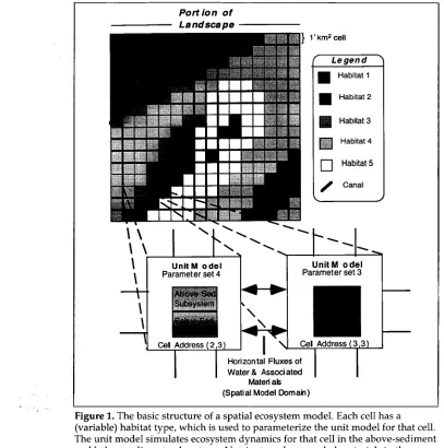
Figure

1. The basic structure of a

_spatial

_ecosystem model. Each cell has a

(variable)

habitat _type, which is used to

_parameterize

the unit model for that cell. The unit model simulates _ecosystem

_dynamics

for that cell in the above-sediment

and below-sediment

_subsystems.

Nutrients and

_suspended

materials in the surface water and saturated sediment water are fluxed between cells in the domain of the

_spatial

model.

computer systems.

Although

the

_importance

of advances in the

_{parallel processing}

field have been

recognized

in the field of

_{spatial modeling}

_[4],

the

conceptual complexity

involved in

_{building complex}

models in a distributed

_{computational}

environment remains a

_major

barrier to the utilization of these

systems

in the environmental sciences. We _propose

to address this issue

_through

the

_development

of a

spatial

modeling

environment to

_support

_ecological/

economic

_(or

other,

e.g.,

biological/social/physical)

model

_development

for state-of-the-art

_parallel

and serial

_computer

_systems.

This

_system,

which links

graphical

tools for

_developing

self-contained

compo-nent models with module databases and

_parallel

code

_generators,

will

_support

modular,

reusable model

_development,

and allow scientists to utilize state-of-the-art

_parallel

_processing

architectures without

investing

unnecessary time in

computer

programming.

2.

_{Spatial Ecosystem Modeling}

We define a

_{dynamic spatial}

model as _any

formula-tion that describes the

_changes

in a

_spatial

_pattern

from time t to a new

_spatial

_pattern

at time t + _1, such that

where

_X(t)

is the

_spatial

_pattern

at time t and

_Y(t)

is a

set of _{array, vector,} or scalar variables that may affect

the transition.

_Although

_{many forms of}

_dynamic

spatial

modeling

are utilized within the broad field of

ecology

[3],

and the

_{spatial modeling}

tools described here are

applicable

to a wide _range of

_modeling

tasks

in the

_biological,

social, economic,

and

_physical

sciences, our

_primary

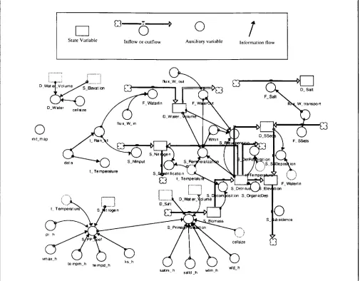
focus in this paper is on

Figure

2. STELLA

_diagram

of the unit model used for the CELSS

_landscape

model.

simulate

_spatial

structure

_by

first

compartmentaliz-ing

the

_landscape

into some

_geometric

_design

and

then

_describing

flows within

_compartments

and

spatial

processes between

compartments

according

to

_{location-specific algorithms;}

see

_Figure

1.

Ex-amples

of

_{process-based, spatially}

articulate land-scape models include wetland models

[2, 5-9],

oceanic

_plankton

models

_[10],

coral reef

_growth

models

_[11],

and fire

_ecosystem

models

_[12].

One

_example

of a

_{process-based spatial}

simulation

model is the

_{Everglades Landscape}

Model

_(ELM),

discussed in Section 3. Another

_example

is the Coastal

_{Ecological Landscape Spatial}

Simulation

(CELSS)

model,

which consists of _2,479 intercon-nected

cells,

each

_representing

1

km2,

constructed for the

_{Atchafalaya/ Terrebonne}

_{marsh/ estuarine}

complex

in south Louisiana

_{[2, 5].}

Each 1 km2 cell in

the CELSS model contains a

_dynamic,

nonlinear

ecosystem

simulation model with seven state

vari-ables,

similar to the one shown in

_Figure

2. The

model is

_generic

in structure and can

_represent

one of

six habitat

_types

_by

_{assigning unique}

_parameter

settings.

Each cell is

_potentially

connected to each

adjacent

cell

_by

the

_exchange

of water and materials. This model is _{several years old} and is much

_simpler

than many models in use

_today.

The

_original

CELSS model took four

_people

about four years

(sixteen

person-years)

to

_fully

_develop

and

implement

using

a

_{supercomputer.}

The model has

proved

to _{be very effective} at

_helping

us understand

complex

ecosystem

behavior and

_{guiding policy}

and research

_{[2, 5].}

We are now concerned with

_reducing

the time involved for both

_developing

and

_running

this

_type

of

_model,

and

_moving

the

_modeling

to

smaller,

less

_expensive

_computers.

Toward that

end,

3.

_{Everglades Landscape}

Model

The

_Everglades

_Landscape

Model

_(ELM)

_[13]

has been

_{developed by}

researchers at the

_University

of

Maryland

using

the

_{Spatial Modeling}

Environment,

Version 1; see Section 6. The ELM is

_designed

to be

one of the

_principal

tools in a

_systematic

analysis

of

the

_{varying options}

in

_managing

the distribution of

water and nutrients in the

_Everglades.

Central to

these

_objectives

is the

_prediction

of

_vegetation

_change

under different scenarios. Water

_quantity,

and the associated

_hydroperiod,

has been a central issue in

understanding changes

to

_vegetation

of the

Ever-glades

[14, 15].

Nutrients from

_agricultural

areas also

appear to be

important

in

_{understanding}

_vegetation

succession

_[16]

in this

_{historically oligotrophic}

system

[17].

The interaction of these

factors,

includ-ing

the

_frequency

and

_severity

of

_fires,

_appears to

drive the succession of the

_plant

communities in the

Everglades

[15,18,19].

Thus,

this

_system

has

_myriad

indirect _{interactions, constraints,} and feedbacks that result in

_complex

_ecosystem

structure

_(biotic

and abiotic

_components

and their flow

_pathways)

and function

_(the

modes of interaction and their

_rates).

For this reason, it is critical to

_develop

a

_systems

viewpoint

toward

_{understanding}

the

_dynamics

inherent in that

_ecosystem

structure and function. Part _{of this process} is the

_development

of a

_dynamic

spatial

simulation model. The ELM is that

_analytic

tool.

In this

model,

the

_important

_ecosystem

_processes that

_{shape plant}

communities are simulated within

the

_varying

habitats distributed

_throughout

the

landscape.

The

_{principal dynamics}

within the model

are

_{plant growth}

in _response to available

_sunlight,

temperature,

nutrients, and water; flow of water

_plus

dissolved nutrients in three

dimensions;

fire initia-tion and

_propagation;

and succession in the

_plant

community

in _response to the environment.

_Using

a mass balance

_approach

in

_{incorporating}

process-based data of a

_{reasonably high}

resolution within the

entire

_{Everglades landscape, changing spatial}

_patterns

and processes can be

_analyzed

within the context of altered

_management

_strategies.

_{Only by}

_{incorporating}

spatial

articulation can an

_ecological

model

realisti-cally

address

_large-scale

_management

issues within the vast,

_{heterogeneous}

_system

of the

_Everglades.

For the

_{spatially explicit}

_ELM, the modeled land-scape is

partitioned

into a

_spatial

_grid

of

_10,178

square unit

cells,

each

having

1 km2 surface area. The

ELM is hierarchical in _structure,

_{incorporating}

an

ecosystem-level &dquo;unit&dquo;

model

_[20]

that is

_replicated

in each of the unit cells

_representing

the

_Everglades

landscape.

The unit model itself is divided into a set

of model sectors that simulate the

_important

ecologi-cal

_{(including physical)}

_dynamics

_using

a

process-oriented,

mass balance

_approach.

While the unit model simulates

_ecological

_{processes within} a unit

cell,

horizontal fluxes across the

_landscape

occur

within the domain of the SME. Within this

_spatial

context, the water _{fluxes between cells carry} dis-solved

_nutrients,

_determining

water

_quantity

and

quality

in the

_landscape.

4.

_{Conceptual Complexity}

and Model

_Development

Development

of

_ecosystem

models in

_general

has been limited

_by

the

_ability

_{of any}

_single

team of researchers to deal with the

_{conceptual complexity}

of

formulating, building, calibrating,

and

_debugging

complex

models. The need for collaborative model

building

has been

_recognized

in the environmental sciences

_{[21, 22].}

Realistic

_ecosystem

models are

becoming

much too

_complex

for _any

_single

_{group of} researchers to

_{implement single-handedly,}

_requiring

collaboration between

_species

_specialists,

hydrolo-gists,

chemists,

land managers, economists,

ecolo-gists,

and others. The current

_generation

of models tends to be

_{idiosyncratic}

monoliths that are

compre-hensible

_only

to the builders

_[22].

_{Communicating}

the structure of the model to others can become an

insurmountable obstacle to _{collaboration and} accep-tance of the model.

_Policy

makers are

_unlikely

to trust a model

_they

do not understand.

A

_{well-recognized}

method for

_reducing

_program

complexity

involves

_structuring

the model as a set of distinct modules with well-defined interfaces

_[21-26].

Modular,

hierarchical model

_structuring

is well

developed

in the context of discrete-event

_modeling

[27, 28],

but has received

_{comparatively}

little

devel-opment

in the realm of continuous

_modeling

_[21,

26,

29]. Ecosystem

models with a modular hierarchical

structure should be closer to natural

_ecosystem

structure than

_procedural

models

_{[21, 26],}

since the

component

populations

of

_ecosystems

are themselves

complex

hierarchical

_systems

with their own internal

dynamics.

Modular

_design

facilitates collaborative model _{construction,} since teams of

_specialists

can

work

_{independently}

on different modules with

minimal risk of interference. Modules can be

archived in distributed libraries to serve as a set of

templates

to

_speed

future

_development.

The

inherit-ance

_property

of

object-oriented languages

allows the

properties

of

_{object-modules}

to be utilized and modified without

_editing

the archived

_object.

A

modeling

environment that

_supports

_modularity

could

_provide

a universal

modeling language

to

module is

_{represented diagramatically,}

so that new users can

_recognize

the

_major

interactions at a

_glance.

Scientists with little or no

_{programming experience}

can

_{begin building}

and

_running

models almost

immediately.

Inherent constraints make it much easier to

_generate

_bug-free

models. Built-in tools for

display

and

_analysis

facilitate

_{understanding,}

debug-ging,

and calibration of the module

_dynamics.

One

_{major advantage}

of this

_{graphical approach}

to

modeling

is _{that the process of}

_modeling

can become

a

_{consensus-building}

tool. The

_graphical

representa-tion of the model can serve as a blackboard for group

brainstorming, allowing policy

makers,

scientists,

and stake-holders to all be involved in the

_modeling

process. New ideas can be tested and scenarios

investigated using

the model within the context of group discussion as the model grows

through

a

collaborative process of

exploration.

When

_applied

in

this manner, the process of

_creating

a model may be more valuable than the finished

_product.

5.

_{Computational Complexity}

and Parallel

_Processing

Tremendous

_{computational}

resources are

_required

to

integrate

the

_equations

of a

_{large spatial}

model in a

reasonable amount of

_computer

time.

_Large

models

typically

require

supercomputers

for efficient

execu-tion. This class of models is a near-ideal

_application

for

_parallel

_processing

since a

_typical

model consists of a

_large

number of cells that can be simulated

semi-independently.

Each processor can be

_assigned

a

different subset of

cells,

and most

_{interprocessor}

communication is

_{nearest-neighbor only.}

_Despite

their

_great

_promise

and

_increasing

_{availability,}

parallel

architectures have not _{found much usage} in the life sciences. The

_major

barrier to wide

_acceptance

of these

_techniques

has been the

_difficulty

_of

pro-gramming

and

_{debugging large parallel}

_programs, and reluctance on the

_part

of scientists to invest time in

_learning

new

_languages

and architectures.

High-performance

computing

must be

_transparent

in order to be

_generally

accessible. The user should

not be concerned with the details: on what

_platform

the simulation is

_running

or how the simulation is

being

farmed out to _{different processors. These}

details are handled

automatically by

the environment

without the user’s

_knowledge

or intervention.

Supporting

transparent

distributed

_computing

for

spatial modeling,

however,

requires

infrastructure

development,

as described later in this paper.

6.

_{Geographic Modeling}

Environment

In an

_attempt

to address the

_conceptual

and compu-tational

_complexity

barriers to

_dynamic

_geographic

model

_development,

we have

_developed

the

_Spatial

modeling

environment

_(SME),

which links icon-based

_{graphical modeling}

environments with

_parallel

supercomputers

and a

_generic

_object

database

_[30,

31].

This

_system

will allow users to create and share

modular,

reusable model

_components,

and utilize advanced

_parallel

_computer

architectures without

having

to invest _unnecessary time in

_computer

programming

or

_learning

new

_systems.

The

follow-ing

sections

_give

a brief

_description

of the current

design

of the SME. A more detailed

_description

can

be found in _{the web page}

_[31].

The SME

_design

has arisen from the need to

support

collaborative model

_building

_among a

_large,

distributed network of scientists involved in

_creating

a

global-scale ecological/economic

model. Its

design

should

_eventually

be

_{general enough}

to

_support

most

large-scale modeling

tasks within the

_biological/

environmental sciences. In the interest of

_maximizing

accessibility

to a distributed network of

_{collaborators,}

the

_system

is

_designed

to

_support

a _{range of}

plat-forms,

both in the front-end

_development

environ-ment and in the back-end distributed network of

platforms.

Since our

goal

is to

_support

_modularity

in model

_design

and

_separate

the

_{implementation}

of the model

_dynamics

from the details of simulation code

development,

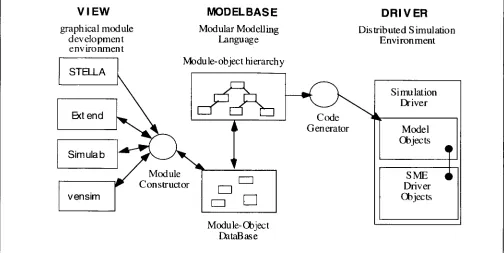
it _{has been necessary} to abstract the module libraries from both the front-end and the back-end environments. We are thus led to the formulation of a

_three-part

ModelBase-View-Driver

architecture;

see

_Figure

3. The three

_components

are

described below.

6.1 View

The View

_component

of the SME is used to

graphi-cally

construct,

calibrate,

and test

biological/ecologi-cal modules. This

_component

is

_{represented by}

an

off-the-shelf

_{graphical modeling}

environment such as

STELLA, Simulab,

or Extend.

6.2 ModelBase

In the next

_step

toward

_constructing

a

_spatial

model,

the Module Constructor translates the View

ecosys-tem

_component

modules into Module

_objects

defined in our text-based Modular

_Modeling

_Language

(MML).

The MML

_objects

can then be archived in the

ModelBase to be accessed

_by

other

researchers,

and/

or used

immediately

to construct a

working spatial

simulation.

_Many

MML

_objects

can be combined

hierarchically

in the MML. This MML

_hierarchy

can

then be converted

_by

the Code Generator into a C++

object hierarchy

within the

_Spatial

_Modeling

Environ-ment

_(SME),

where it can drive a

spatial

simulation.

The MML is

_designed

to

_capture

_only

the relevant

dynamics

of the simulation module

_being

constructed,

Figure

3. Overview of the ModelBase-View-Driver architecture

For

_example,

the features that can be

represented

in

the MML include

_dynamics

of

_growth,

death,

and transformation of

_{biological/ecological}

_entities,

fluxes of water, nutrients,

pollutants,

etc., and the internal decision and

_learning

_{processes of}

_biological

agents.

The features that are not

_represented

in the MML include the

_{spatio-temporal implementation}

of the

model,

input

and

_output

of model

data,

and the distribution of the model over a set _{of processors.}

These features are

_{implemented by}

the Code

Genera-tor and the simulation

drivers;

see the next sections. 6.3 Code Generators

The Code Generators convert an MML

object

hierar-chy

into a C++

object hierarchy

that is

_incorporated

into the simulation driver

_application

to create a

spatial

simulation. The user customizes the set of

objects generated by

entering

information into a set

of

_{configuration}

files that are

_{initially generated by}

the Code Generator. In the final version a

menu-driven interface will be

_provided

to facilitate this

configuration

step.

During

the

_{configuration}

_step

the user

_specifies

the

additional information that is

_required

to transform the MML

_object

into a

_dynamic

simulation

_object.

The information entered falls into several

_general

categories:

(1)

Space-Time

Implementation.

In this

_step,

each MML

object

is associated with a

frame,

which

_specifies

its

_space-time

_{implementation.}

A frame is a C++

object

that

_specifies

the

_topology

of the

_spatial

implementation

of the

module,

methods for

interacting

with and

_transferring

data to other

frames,

and

_temporal

methods for

_handling

the

passing

of time. The driver

_geometry

_object

(Figure

6)

maintains a

_catalog

of available frames.

Examples

of available frames include

two-dimensional

_{grids (e.g.,}

for

_landscapes),

_graphs

and networks

_(e.g.,

for river,

canal,

or neural

networks),

and

_agents

_(e.g.,

for individual

_agents

moving

about in the

_landscape).

The user

_specifies

a

frame

_type

as well as a

(set of)

GIS

map(s)

that the

frame will read at runtime to

_configure

itself.

(2) Input/Output Configuration.

In this

_step

the user

configures

input

to the simulation from the

biological/ ecological

databases and GIS.

_Input

configuration

must be done at code

_generation

time because the Code Generator uses this

information

_(together

with the variable

depen-dency graph)

to determine variable

_types.

_Output

configuration

is done at _runtime,

_although

default values can be

_specified

in the CG

_{configuration}

files. 6.4 PointGrid

_Library

The PointGrid

_{Library (PGL)}

is a set of C++ distributed

objects designed

to

_support

_computation

on

irregular,

distributed networks and

_grids.

It contains the core set

of

_objects

on which the SME Driver is constructed. The

PGL

_object

structure is a direct

_mapping

of an

_early

Figure

4. Structure of the SME.2 simulation driver as discussed in _{the web page}

_[31].

The PGL builds

_spatial

_{representations}

from sets of

Point

_objects

_{(see below)}

with links. It

_{transparently}

handles:

₍₁₎

creation and

_{decomposition}

_(over

processors)

of

_PointSets,

₍₂₎

_mapping

of data over

and between

_PointSets,

₍₃₎

iteration over PointSets

and Point

Sub-Sets,

(4)

data access and

update

at

each _Point, and

₍₅₎

_swapping

of variable-sized PointSet

_{boundary (ghost)}

_regions.

Some of the

important

ML classes are listed below.

. point:

_Corresponds

to a cell in a GIS

_layer.

aggregates

Point:

_Corresponds

to a cell in a coarser

resolution GIS

_layer.

· PointSet: A set of Points with links

_(grid

or

_network).

· DistributedPointSet: A PointSet distributed over

processors with variable-sized

boundary (ghost)

layers.

· Coverage:

Mapping

from a DistributedPointSet to

the set of floats.

6.5 Driver

The SME Driver

_(Figure

₄₎

is a distributed

object-oriented simulation environment that

_incorporates

the set of code modules that

_{actually perform}

the

spatial

simulation on the

_{targeted platform.}

It is

implemented

as a set of distributed C++

_objects

linked

_by

_message

_passing.

Of all the

_objects

shown in

_Figure

_4,

_only

the interface

_object

is visible to the

user; the rest will

_perform

their tasks

_{automatically}

and

_invisibly.

The

_major

driver

_components

include

the

_following.

· Application Object:

Handles

_general

_process of simulation execution and coordination and

sched-uling

of the other SME

_objects.

· Imported Objects

and Data: This is the set of

_objects

and data that is created

_by

the Code Generator and

imported

into the driver. The

_objects

are C++

implementations

of the ModelBase modules. The

imported

object

structure is described in more

detail below.

· Geometry

Object:

Maintains the

_catalog

of frames

(see

Section

_7.3)

and handles all tasks

_relating

to

the

_{spatial configuration}

of the

_simulation,

such as

translating/

transferring

data between frames and the network

_object.

. Network

_Object:

Handles communication between processors and the simulation host. It is

implemented

using

the MPI _message

_passing

interface standard

_[33].

· Interface Object:

Menu-driver interface

_facilitating

user control of the simulation and real-time

_display

of simulation

_output.

Provides the user with a

single

familiar environment in which to interact with simulations

_running

on _{any one of} a number

of

_parallel

or serial

_computers.

- File

Object:

Handles

_archiving

of simulation

_output

in HDF format. Later versions will

_actively

The

_imported

_objects

are built _{upon the}

following

classes:

. Module Class: The CodeGenerator

_Application

converts each module in the MML model

descrip-tion into a Module

_Object

in the Driver. Each Module

_Object

has a set of Variable

_Objects

and a

Frame

_Object.

It also has a set of methods for

responding

to simulation events such as &dquo;Initialize&dquo;

and

_{&dquo;Update.&dquo;}

· Frame Class: A Frame

_Object

is a driver

_object

that

_specifies

the

_topology

of the

_spatial

implemen-tation of a Module

_{Object, including}

methods for

interacting

with and

_transferring

data to other frames. A frame has a list of Point

Objects

(POs),

with each PO

_{corresponding}

to a cell in the frame’s

map

region,

which includes a

_partition

of the

study

area handled

_by

the current _processor

_plus

a

communication buffer zone. The driver maintains a

catalog

of available

frames,

which includes

two-dimensional

_{grids (e.g.,}

for

_{landscapes), graphs}

and networks

_(e.g.,

for river,

canal,

or neural

networks),

areas

_(e.g.,

for embedded

_{lumped-parameter}

models),

and

_point

collections

_(e.g.,

for individual

agents

moving

about in the

_landscape).

. Variable Class: The CodeGenerator

_Application

converts each variable declared in the MML model

description

into a Variable

Object

in the Driver.

The Variable class is a

_{specialization}

of the

Cover-age

class,

which

encapsulates

a

_mapping

from the

set of Point

_Objects

owned

_by

the Module’s Frame

Object

into the set of

_floating

_point

numbers.

6.6 User

_Interface

The SME user

interface,

which is

_currently

under

development

using

the

_Tcl/Tk

_scripting

_language

[34],

will

_provide

the user with a

_single

familiar

environment in which to build and run simulations on _{any one of} a number of

_parallel/

distributed or

serial

_computers.

This

_{user-friendly}

_environment, with

_{hierarchically}

structured interaction

_levels,

will allow users with

_widely

_varying

_goals

and

back-ground knowledge

(from

scientists and students to

policy makers)

to

build,

configure,

and run

_spatial

simulations,

and to

_generate

_graphical

_output

in a manner

_appropriate

to their level of

_expertise.

The lowest level of interface to the SME is

_{expedited by}

a

tcl shell. In the

_{SME/ tcl}

shell environment the user can create new

_projects,

customize the

_SME,

and run

the various SME

_{subapplications.}

Three menu-driven

tcl/tk

applications

are

_{being developed}

for

₍₁₎

config-uring

the Driver and code

_generators,

₍₂₎

_controlling

the simulation and

_visualizing

the simulation

_output,

and

₍₃₎

_building

models in MML.

6.6.1 Simulation

_{Configuration Interface.}

All simulation IO is

_{accomplished using &dquo;pipe&dquo; objects,}

_e.g., the real-time screen

_display

of a variable’s

_spatial

data is rendered

_by

_configuring

a

_pipe

_object

to connect the

spatial

variable with a _map animation

_object.

The

user interface

_provides

a menu-driven tool for

configuring

pipes

for

₍₁₎

_map

_input

from

GIS,

₍₂₎

parameter

input

from relational

databases,

(3)

map

output

to _GIS,

₍₄₎

assorted data

_input/output

_to/

from disk

archives,

and

₍₅₎

various

_types

of real-time

display, including

map animations,

graphs,

and tables. This interface also allows the user to

_configure

various

parameters

associated with each simulation

_object.

6.6.2 Simulation

_Object

Browser and Viewer. A

_separate

tcl/ tk

application

allows the user to browse

_through

the

_objects

in a

_paused

simulation and view each

object’s

internal data structures in a convenient format. The browser also

_provides

a menu of each

object’s dependent objects,

so users can

quickly

traverse the

_dependency

tree while

_searching

for anomalies in the simulation

_output.

This

_application

incorporates

the viewers that are used for real-time

display

of simulation

_output.

6.6.3 Icon-Based Model

_{Development Interface.}

A third interface

_component

is under

_development

to

pro-vide an icon-based interface to the ModelBase

component

of the SME, to facilitate simulation module

_development

and

_{linking/ archiving}

in the Modular

_Modeling

_{Language (MML).}

This interface

provides

a

_graphical

_mapping

of each

_component

of

the MML

_{language, allowing}

modelers to create

MML modules in a

_{user-friendly,}

visual

environ-ment. The environment _{enforces proper} MML

_syntax

and model

_{design, provides}

a blackboard for

collabo-rative model

_development,

and also

_provides

on-line

help

screens to document each

_component

of the MML

_language.

6.7

_{Linking Existing}

Simulation Code with the SME In order to create a new module in the _SME, one

must

_develop

it in the View

_{graphical modeling}

environment or the MML. There is a wealth of

complex

simulation code in existence in the world

today,

written

_mainly

in FORTRAN or

C,

that would

be too difficult to

_completely

rewrite in the MML or a

View-supported language (although

this

_might

be the

_optimal

_approach,

_manpower

_permitting).

Therefore,

we are

_developing

a stand-alone version of the network

_{object displayed}

in

_Figure

4 that will form the core of an &dquo;SME

wrapper.&dquo;

This

&dquo;wrapper&dquo;

is a

_library

of FORTRAN or C functions that a

code to

_give

it the

_ability

to interact and

_exchange

data with the SME over the Internet. Once the

wrapper is

incorporated

into the

legacy

simulation

code,

then SME variables can be linked with

legacy

variables

_using

_{simple configuration}

commands. The SME and the

_legacy

code can be run

simulta-neously

and can feed information back and forth across the Internet. For

_example,

an SME

_landscape

simulation

_might

wish to link with an

_existing

hydrodynamics

simulation to handle the

hydrody-namics of the watershed.

7. Simulation

_Development

in the SME

Realistic

_spatial

models are

_{extremely complex,}

requiring

large

quantities

of

data,

so that

_designing,

calibrating,

and

_validating

these models is a difficult

task. The

_development

of a

_spatial

simulation occurs

in three

_stages:

₍₁₎

_non-spatial

module

_development,

(2)

non-spatial

model

_{development (linking}

mod-ules),

and

_{(3) spatial}

model

_development.

7.1 Simulation

_Design

The simulation

_design

_process occurs

_primarily

in the View

_component,

where the simulation unit modules

are created.

Thus,

the vast

_majority

of the

_design

work occurs in the

_non-spatial

_regime,

_involving

concepts

and processes that are familiar to most

modelers.

_Typically

a _{group of modelers will work}

together

on a set of

_closely

related

modules,

with

prior

agreement

on the set of available

_outputs

from each module. Once

_developed

and tested in the View

environment, the modules are then linked in the

View or ModelBase environment for a further round

of tests.

_Implementing

the

_spatial

interactions can occur

_{by designing}

these interactions in the MML

language,

or

_{by linking predefined}

methods from the

SME Driver libraries. Libraries have been

_developed

to

_implement

common

_hydrologic

scenarios,

includ-ing

movement of water and constituents over and

under the

_landscape

surface. The

_{spatial dynamics}

are tested in the SME Driver environment. 7.2 Calibration and

_Verification

The simulation calibration _{and verification process} involves three

_phases:

. Phase 1: The unit modules are calibrated

individu-ally

and

_{non-spatially}

in the View environment. . Phase 2: The assembled unit model is calibrated and

verified

_{non-spatially}

in either the View or the

Driver environment.

. Phase 3: The full unit model is calibrated and verified

_spatially

in the Driver environment. The final

_stage

of calibration involves

_only

the

_spatial

aspects

of the

simulation;

all calibration that can be

accomplished

without reference to the

_spatial

nature of the

_system

is

_completed

in

_phases

1 and 2. Due to data limitation, most calibration and verification in

_phase

3 is

_{accomplished using}

sets of

&dquo;integrators,&dquo;

i.e., localized

_quantities

whose

dynam-ics

_depend

on a number of

spatial

_processes. For

example,

river flux rate and nutrient concentrations may be measured at a number of stations

_along

a

river. These data

_{play a}

_major

role in

_calibrating

and

verifying

a number of

spatial

_processes that influence

the movement of water and nutrients across the

landscape

and into the river.

8. Conclusions

Parallel

_computer

hardware and software are now

well

_{developed enough}

to allow their use in

large-scale

_biological

and environmental

_modeling.

Parallel

systems

are

particularly

well suited to

_spatial

model-ing,

allowing relatively complex

unit models to be executed over a

relatively high-resolution spatial

array at reasonable cost and

speed.

When linked with icon-based

_graphical

model

_development

tools and

GIS/database

tools,

one has a

powerful

_yet

easy-to-use

_{spatial modeling}

environment.

In

_addition,

the

_widespread

use of

_object-based

modeling

environments linked

_{transparently}

to

state-of-the-art distributed

_computing

resources could

result in a fundamental

_paradigm

shift in

_complex

systems

modeling.

The

_modeling

formalism

_imposes

the constraints of

_modularity

and

_hierarchy

in program

design.

General

adoption

of this

paradigm

will

_support

the

_development

of libraries of modules

representing

reusable model

_components

that are

globally

available to model

_builders,

as well as make

advanced

_computing

architectures available to users

with little

_computer

_knowledge.

We believe that

_effectively

_managing

human affairs

_through

the next

_century

will

_require

ex-tremely complex

and reliable

_computer

models.

Widespread

utilization of

_modeling

environments

9.

References

[1] Risser, P.G., Karr, J.R., and Forman, R.T.T. 1984.

Landscape

Ecology:

Directions and

_Approaches.

Illinois

Natural

_{History Survey,}

_Champaign,

IL.

[2]

Costanza, R., Sklar, F.H., and White, M.L. 1990.

"Mod-eling

coastal

_{landscape dynamics."}

BioScience vol. 40,

pp. 91-107.

[3]

Sklar, F.H. and Costanza, R. 1991. "The

_development

of

dynamic spatial

models for

_{landscape ecology."}

Quantitative Methods in

_{Landscape Ecology.}

Turner, M.G.,

and Gardner, R., eds. New York:

_{Springer-Verlag.}

[4] Casey,

R.M. and _Jameson, D.A. 1988. "Parallel and

vector

_processing

in

_{landscape dynamics."}

_Applied

Mathematics and

_Computation

vol. 27, pp. 3-22.

[5]

Sklar, F.H., Costanza, R., and

_Day,

_J.W.J. 1985.

"Dy-namic

_spatial

simulation

_modeling

of coastal wetland habitat succession."

_{Ecological Modeling}

vol. 29, pp. 261-281.

[6]

Costanza, R., Sklar, F.H., and

_Day,

J.W. 1986.

"Model-ing

spatial

and

_temporal

succession in the

_Atchafalaya/

Terrebonne

_{marsh/estuarine complex}

in South Louisi-ana." Estuarine

_Variability.

Wolfe, D.A., ed., New York: Academic Press.

[7]

Kadlec, R.H. and Hammer, D.E. 1988.

_"Modeling

nutrient behavior in wetlands."

_{Ecological Modeling}

vol.

40, pp. 37-66.

[8] Boumans, R.M.J. and _Sklar, F.H. 1991. "A

polygon-based

_spatial

model for

_{simulating landscape change."}

Landscape

Ecology

vol. 4, pp. 83-97.

[9] White, M.,

_Day,

D., Maxwell, T., Costanza, R., and

Sklar, F. 1992.

_{"Ecosystem modeling Utilizing desktop}

parallel

computer

technology."

Hydraulic

and Environ-mental

_Modeling:

Estuarine and River Waters. _Falconer, R.,

ed.

_Ashgate.

[10]

Show, LT., Jr. 1979. "Plankton

_community

and

physical

environment simulation for the Gulf of Mexico

region." Proceedings of

the 1979 Summer

_Computer

Simulation

_Conference.

The

_Society

for

_Computer

Simulation _{International. pp. 432-439.}

[11] Maguire,

L.A. and Porter, J.W. 1977. "A

_spatial

model of

_growth

and

_{competition strategies}

in coral communi-ties."

_{Ecological Modeling}

vol. 3, pp. 249-271.

[12] Kessell, S.R. 1977. "Gradient

_modeling:

A new

approach

to fire

_modeling

and resource

_management."

Ecosystem Modeling

in

_Theory

and Practice. Hall, C.A.S. and

_Day,

_J.W.J., eds. New York:

_{Wiley-Interscience.}

[13]

Fitz, H.C., Costanza, R., and

_Reyes,

E. 1993. The

Everglades Landscape

Model

_(ELM).

South Florida Water

Management

District,

_Everglades

Research Division.

[14]

Davis, S.M. 1994.

_{"Phosphorus inputs}

and

_vegetation

sensitivity

in the

_{Everglades." Everglades:}

The

_Ecosystem

and Its Restoration. Davis, S.M. and

_Ogden,

_J.C., eds.

Delray

Beach, FL: St. Lucie Press.

[15]

White, P.S. 1994.

_"Synthesis:

_Vegetation

_pattern and process in the

Everglades ecosystem." Everglades:

the

Ecosystem

and Its Restoration. Davis, S.M., ed.

_Delray

Beach, FL: St. Lucie Press.

[16]

Davis, S.M., 1991. "Growth,

_{decomposition}

and

nutrient retention of cladium

_jamaicense

crantz and

typha domingensis

pers. in the Florida

_Everglades."

Aquatic Botany

vol. 40, pp. 203-224.

[17]

Steward, K.K. and Ornes, W.H. 1975. "The

_autecology

of _sawgrass in the Florida

_{Everglades." Ecology}

vol. 56,

pp. 162-171.

[18] Duever, M.J. 1984. "Environmental factors

_controlling

plant

communities of the

_{Big Cypress Swamp."}

Environments

_of

South Florida: Present and Past. _Gleason,

P.J., ed. Miami, FL: Miami

_Geological

_Society.

[19]

Gunderson, L.H. 1989. "Historical

_{hydropatterns}

in wetland communities of

_Everglades

National Park."

Freshwater Wetlands and

_Wildlife

vol. _{61, pp.} 1099-1111.

[20]

Fitz, H.C., DeBellevue, E., Costanza, R., Boumans, R., Maxwell, T., and

_Wainger,

L. 1995.

_"Development

of a

general

ecosystem model

_(GEM)

for a _range of scales

and

_{ecosystems." Ecological Modeling}

vol. 88, pp.

263-297.

[21]

Goodall, D.W. 1974. The Hierarchical

_Approach

to Model

Building.

Wageningen:

Center for

_Agricultural

Publish-ing

and Documentation.

[22]

Acock, B. and

_Reynolds,

_J.F. 1990. "Model structure

and data base

_{development."}

Process

_{Modeling of}

Forest Growth

_Responses

to Environmental Stress. Dixon, R.K., Meldahl, R.S., Ruark, G.A., and Warren, W.G., eds.

Portland, OR: Timber Press.

[23] Gauthier, R.L. and Ponto, S.D. 1970.

_Designing

_Systems

Programs. Englewood

Cliffs, NJ: Prentice-Hall.

[24]

Tichenor, L.H. 1989. "Modular simulation of the static

portions

of the leaf

_budget.

SIMULATION vol. 55, pp. 345.

[25]

Hodges,

T., Johnson, S.L., and _Johnson, B.S. 1992. "A modular structure _{for crop simulation models."}

Agronomy

Journal vol. 84, pp. 911-915.

[26] Silvert, W. 1993.

_{"Object-oriented}

_ecosystem

model-ing." Ecological Modeling

vol. 68, pp. 91-118.

[27]

Zeigler,

B.P. 1976.

_Theory

_{of Modeling}

and Simulation. New York: _John

_Wiley

& Sons.

[28]

Zeigler,

B.P. 1990.

_{Object-Oriented}

Simulation with

Hierarchical, Modular Models. New York: Academic Press.

[29]

Cellier, F.E. 1991. Continuous

_System

_Modeling.

New York:

_{Springer-Verlag.}

[30]

Maxwell, T. and Costanza, R. 1995. "Distributed

modular

_spatial

_ecosystem

_modelling."

International

Journal

of

Computer

Simulation:

_Special

Issue on Advanced

Simulation

_{Methodologies}

vol. 5, no. 3, pp. 247-262.

[31]

SME2:

_{Spatial Modeling}

Environment, version 2

_alpha.

1995. URL:

_{http://kabir.umd.edu}

_/SMP/MVD/

SME2.html.

[32] OGIS: The

_OpenGIS

Guide. 1996. URL:

_{http://ogis.org/}

guide/ guidel.htm.

[33] MPI:

_Message

_{Passing Interface.}

1995. URL:

_http://

www.mcs.anl.gov/mpi/index.html.

THOMAS P. MAXWELL received his Master’s

_degree

in

Physics, focusing

on chaos

_theory

and nonlinear

_dynamics,

in 1983, and his PhD in

_Physics,

_focusing

on neural

networks,

_parallel

processing,

and artificial

_{intelligence,}

in

1988. He has

_developed

neural network architectures for

image processing,

pattern

recognition,

adaptive

control,

associative _{memory, and} artificial

_intelligence

_{applications.}

For the last five _years he has been

_developing

_spatial

ecosystem models and simulation environments for the International Institute for

_Ecological

Economics. A

_major

focus of this work has been the

_development

of collaborative tools to _support modular

_{spatiotemporal}

modeling

in distributed

_{computational}

environments. He

has worked as a consultant for NASA, several of NASA’s

contractors, the

_University

of Louisiana, and the

University

of Illinois.

ROBERT COSTANZA is Director of the

_University

of

Maryland’s

International Institute for

_Ecological

Economics, and a

_professor

in the Center for Environmental and Estuarine Studies,

University

of

Maryland System,

Solomons, MD. He is also Director of

the

_complex

_{systems research program} at

_Beijer

International Institute of

_Ecological

Economics, The

_Royal

Swedish

_Academy

of Sciences, Stockholm, Sweden. He received his PhD from the

_University

of Florida in

_Systems

Ecology

with a minor in Economics. He is cofounder and

president

of the International

_Society

for

_Ecological

Economics

_(ISEE)

and chief editor of the

_{Society’s journal:}

Ecological

Economics. In 1992 he was awarded the

_Society

for Conservation

_Biology

_{Distinguished}

Achievement Award, and in 1993 he was selected as a Pew Scholar in Conservation and the Environment.

Dr. Costanza’s research has focused on the interface

between

_ecological

and economic _systems,

_particularly

at

larger temporal

and

_spatial

scales. This includes

_landscape

level

_spatial

simulation

_modeling,

_analysis

of _{energy flows}

through

economic and

_ecological

_systems, valuation of