Short-term Sparse Portfolio Optimization Based on
Alternating Direction Method of Multipliers
Zhao-Rong Lai [email protected]
Department of Mathematics Jinan University
Guangzhou 510632, China
Pei-Yi Yang [email protected]
School of Mathematics Sun Yat-Sen University Guangzhou 510275, China
Liangda Fang [email protected]
Xiaotian Wu [email protected]
Department of Computer Science Jinan University
Guangzhou 510632, China
Editor:Qiaozhu Mei
Abstract
We propose a short-term sparse portfolio optimization (SSPO) system based on alternating direction method of multipliers (ADMM). Although some existing strategies have also exploited sparsity, they either constrain the quantity of the portfolio change or aim at the long-term portfolio optimization. Very few of them are dedicated to constructing sparse portfolios for the short-term portfolio optimization, which will be complemented by the proposed SSPO. SSPO concentrates wealth on a small proportion of assets that have good increasing potential according to some empirical financial principles, so as to maximize the cumulative wealth for the whole investment. We also propose a solving algorithm based on ADMM to handle the `1-regularization term and the self-financing constraint simultaneously. As a significant improvement in the proposed ADMM, we have proven that its augmented Lagrangian has a saddle point, which is the foundation of the iterative formulae of ADMM but is seldom addressed by other sparsity strategies. Extensive experiments on 5 benchmark data sets from real-world stock markets show that SSPO outperforms other state-of-the-art systems in thorough evaluations, withstands reasonable transaction costs and runs fast. Thus it is suitable for real-world financial environments. Keywords: short-term portfolio optimization, sparse portfolio, alternating direction method of multipliers
1. Introduction
Portfolio optimization (PO) via machine learning systems has been catching more and more attention recently (Li and Hoi, 2012; Huang et al., 2013; Li et al., 2015; Li and Hoi, 2014; He et al., 2015; Yang et al., 2015; Huang et al., 2016; Li et al., 2016; Mahdavi-Damghani et al., 2017). It aims to invest in a group of financial assets with instructions
c
by the machine, based on some financial principles and optimization strategies. Since it requires a large amount of quantitative calculation, machine learning methods are in high demand to reduce mistakes and biases made by human in real-world investment.
PO originates from the mean-variance theory (Markowitz, 1952), which seeks to min-imize the volatility of a portfolio given a certain expected return level. From then on, various theories based on such a framework are proposed in the language of probability and statistics (Sharpe, 1964; Fama, 1965; Lintner, 1965; Fama, 1970; Treynor and Black, 1973). The equally-weighted portfolio is a popular theory that can achieve good performance if the individual risks of the assets are similar, while the risk parity theory is efficient in di-versifying the portfolio risk if the individual risks are significantly different (Maillard et al., 2010). Instead of treating PO as a static problem, the stochastic portfolio theory (Fernholz, 2002) further extends it to a dynamic problem under some strict statistical assumptions. Besides, some special objectives can be achieved by adding specific prior knowledge into the dynamic model, like the rank-dependent portfolios. However, all the above methods are rather theoretical and their conclusions are based on very strict statistical assumptions that are far from real-world situations. On the other hand, machine learning strategies do not require such strict assumptions, thus they are more productive and effective in a well-defined technical sense (Das et al., 2013; Shen et al., 2014; Ho et al., 2015).
The attempt to construct sparse portfolios via machine learning starts in the long-term PO. In general, a long-term PO changes its portfolio once for a week or a month (or even a year). It focuses on the choice of assets rather than the timing of trading (buying or selling). A kind of sparse and stable Markowitz portfolios (SSMP) is proposed by Brodie et al. (2009). It adds an `1-regularization (Cand`es and Plan, 2009) term of the portfolio vector to the traditional Markowitz model, which regulates the amount of short-position in the portfolio. The regularized symmetric tail average (STA) minimization is proposed by Still and Kondor (2010), which exploits the Karush-Kuhn-Tucker (KKT) conditions (Bertsekas, 1999) to make the portfolio sparse. Ho et al. (2015) also construct sparse mean-variance portfolios with weighted elastic net penalization (Zou and Hastie, 2005). Shen et al. (2014) propose the doubly regularized portfolio allocation to control the quantity of portfolio change. Empirical or simulated experiments indicate that they show some advantages in the long-term PO.
However, few systems construct sparse portfolios for the short-term and online PO, which changes its portfolio once for a day (or even shorter). Since the short-term PO is more general than the long-term PO (e.g., one can change the portfolio only on the first day of each month), the short-term PO considers both of the choice of assets and the timing of trading. While the objective of long-term PO is to minimize the quadratic risk (Markowitz, 1952; Brodie et al., 2009; Ho et al., 2015; Shen et al., 2014), the objective of short-term PO is to maximize the increasing factor on each day and ultimately the cumulative wealth (Cover, 1991; Agarwal et al., 2006; Li et al., 2011; Das et al., 2013; Li et al., 2015; Huang et al., 2016; Li et al., 2016).
public solving schemes. Shen et al. (2014) point out that this problem is difficult and turn to a commercial software for solution. Ho et al. (2015) include the `1-regularization term but exclude the self-financing constraint. Although Das et al. (2013) successfully set up an ADMM algorithm, they do not prove that its augmented Lagrangian has a saddle point, which is the foundation of the iterative formulae of ADMM. In fact, the saddle point proof is also absent in other applications (Mohsin et al., 2015; Zhan et al., 2016) than PO. Besides, not all designs of ADMM have saddle points.
To address the above-mentioned problems, we propose a novel Short-term Sparse PO (SSPO) system based on ADMM. It well fits the machine learning framework for the short-term PO and is free of the strict assumptions of the stochastic portfolio theory. Its novelty falls into several aspects.
• Most state-of-the-art short-term PO systems focus only on adopting empirical finan-cial principles (like the mean reversion) (Li et al., 2012, 2013, 2015; Huang et al., 2016), but SSPO also exploits the intrinsic sparse structure of portfolio by using an `1-regularization term and a self-financing constraint simultaneously, which lacks public solving schemes.
• Most previous sparsity models minimize the square error (Brodie et al., 2009; Still and Kondor, 2010; Lai et al., 2015; Zhan et al., 2016) or the quadratic risk (Brodie et al., 2009; Ho et al., 2015), but SSPO maximizes an increasing factor, which is quite different from the former in formulation.
• Previous sparsity models for short-term PO constrain the quantity of the portfolio change to form “lazy updates” (Das et al., 2013; Shen et al., 2014), which are defensive strategies and not really sparse PO systems. But SSPO actively updates the sparse portfolio according to the changing increasing potential of different assets as time passes, which is an aggressive strategy.
• We prove that the augmented Lagrangian of SSPO has a saddle point, which is the foundation of the iterative formulae of ADMM but is seldom addressed by other sparsity models.
The rest of the paper is organized as follows. Section 2 presents some preliminaries and related works. Section 3 illustrates the whole SSPO system and its solving algorithm. Section 4 presents extensive experimental results to evaluate SSPO. Finally, Section 5 draws conclusions.
2. Preliminaries and Related Works
2.1. Problem Setting of Short-term Portfolio Optimization
We present the framework of short-term PO via machine learning, which is taken as baseline by many previous researches (Cover, 1991; Agarwal et al., 2006; Li et al., 2015; Huang et al., 2016; Li et al., 2016). Suppose there are d assets in a financial market, their prices are collected as a vector pt ∈ Rd+, t = 0,1,2,· · ·, where Rd+ represents the d
sequence. We can evaluate the performance of assets by the price relativext, ppt−1t , where
the division is performed element-wise.
A portfolio is a vector lying on the d-dimensional simplex bt ∈ ∆d := {b ∈ Rd+ :
Pd
i=1b(i)= 1}with assumptions of non-short-selling and self-financing (without borrowing
money and full re-investment). It represents the proportion of the total wealth invested in different assets at the beginning of thet-th period.
At the end of the t-th period, the cumulative wealth St evolves by an increasing factor
of b>t xt: St=St−1·(b>txt). Suppose the whole investment lastsn periods and the initial
wealth is S0 = 1, then the final cumulative wealth is Sn =Qtn=1(b>t xt). The objective of
short-term PO is to maximizeSnby maximizingb>t xton each period (Cover, 1991; Agarwal
et al., 2006; Li et al., 2011; Das et al., 2013; Li et al., 2015; Huang et al., 2016; Li et al., 2016):
ˆ
Sn= max
{bt∈∆d}nt=1 n
Y
t=1
(b>t xt). (1)
Note that no statistical assumptions regarding the movement of asset prices are required in the framework.
2.2. Related Works on Short-term Portfolio Optimization
Different systems or strategies suggest different principles of optimizingbtas time passes.
In general, short-term PO systems need to flexibly react to the rapid change of financial environments, thus they have to exploit some principles of empirical financial studies (Je-gadeesh, 1990, 1991; Li and Hoi, 2014; Li et al., 2016) and investing behaviors (Kahneman and Tversky, 1979; Bondt and Thaler, 1985; Jegadeesh and Titman, 1993) to make future price predictions, rather than follow strict statistical assumptions that may only take effect in the long run (Das et al., 2013). For example, some state-of-the-art short-term PO sys-tems adopt the mean reversion principle in finance (Jegadeesh, 1990, 1991; Li et al., 2012, 2013, 2015; Huang et al., 2016), which indicates that the future price of an asset will reverse to some kind of its historical mean.
2.2.1. Two Trivial Systems
A simple but widely used system is the Uniformly Buy-And-Hold (UBAH) strategy (Li and Hoi, 2014), which disperses the wealth equally in all the assets at the very beginning and remains unchanged: ˆSnU BAH = 1dPd
i=1
Qn
t=1x (i)
t . It is taken by most financial markets
as their market strategies.
On the contrary, the Beststock (BS) strategy (Li and Hoi, 2014) allocates all the wealth to the best performing asset in the whole investment: ˆSnBS = max
b∈∆d
b>(Nn
t=1xt), where
N
is the element-wise product operator. It is a hindsight strategy that cannot be implemented in reality.
2.2.2. Systems Based on Correlation
of different assets by the cross-window correlation cori,j = (lx (i)−lx¯(i)
)>(ly(j)−ly¯(j)
)
klx(i)−lx¯(i)kk
ly(j)−ly¯(j)k and an
anti-correlationAi =|cori,i|ifcori,i <0; elseAi = 0, where k · kis the Euclidean norm, lx
and ly are logarithmic returns in two successive windows.
CORN (Li et al., 2011) further combines correlation with pattern-matching (Gy¨orfi et al., 2006) and searches for historical correlation-similar patterns
Ct+1(w, ρ) =
(
w < k < t: cov(X
k−1
k−w,Xtt−w+1) std(Xkk−−1w)std(Xt
t−w+1)
>ρ
)
,
whereXkk−−1w denotes the price relative vectors in the time window [k−w, k−1].
Mahdavi-Damghani et al. (2017) consider PO in the context of cointelated pairs, a typical model for pairs trading. It is designed to signify a hybrid method between the cointegration and the correlation models. There are two approaches to addressed this problem: Stochastic Differential Equation and Band-wise Gaussian Mixture, which give similar results but the latter keeps the methodology simpler and more adaptable to the regime change.
2.2.3. Systems Based on Average Indices
OLMAR (Li et al., 2015) exploits the popular financial tool of moving average (MA) to predict future asset prices. It is a defensive and moderate strategy with a neutral risk appetite, so as to avoid over-estimating or under-estimating:
ˆ
xt+1(w) =
M At(w)
pt
=
Pw−1
k=0 pt−k
wpt
= 1
w 1+ 1 xt
+· · ·+Nw−12
k=0 xt−k
!
, (2)
where 1 is a vector with elements of 1, whose dimension can be inferred from the context, and w is the window size. Its portfolio update scheme is the same as the below-mentioned RMR strategy (Huang et al., 2016).
RMR also makes moderate price predictions, but substitutes `1-median (Vardi and Zhang, 2000) for MA, since`1-median is more robust to noise and outliers:
ˆ
pt+1 = argmin
p∈Rd+ w−1
X
k=0
kpt−k−pk, ˆxt+1 =
ˆ pt+1
pt
. (3)
Both RMR and OLMAR use the following optimization model to update portfolio:
bt+1 = argmin
b
1 2kb−
ˆ
btk2 s.t.b>xˆt+1> >0, (4)
ˆ
bt+1 = argmin
b∈∆d
kb−bt+1k2. (5)
(5) is a normalization to the simplex (Duchi et al., 2008). This optimization model does not impose sparsity constraints on the portfolio, and it tries to approach the current portfolio ˆ
2.3. Related Works on Sparsity Constraints
Although sparsity models have been proposed for PO, they either aim at the long-term PO or constrain the quantity of the portfolio change. Very few of them aim to construct sparse portfolios for the short-term PO.
2.3.1. Systems for Long-term Portfolio Optimization
Sparse and Stable Markowitz Portfolio (SSMP) (Brodie et al., 2009) uses the following regularization model
bSSM P = argmin
b
k1(n)− Rbk2+τkbk
1 s.t.b>µ=,b>1= 1, (6)
where is a predefined prospective growth rate, 1(n) is an n-dimensional vector of 1, R
is an n×d-dimensional asset return matrix, µ is the expectation of asset returns, k · k1
denotes the`1-Norm, andτ is the regularization strength. Rbcontains the actual portfolio returns of n samples, while b>µ is the expectation of the portfolio return. (6) constrains b>µto a predefined level, and tries to minimize the square error (i.e., the quadratic risk in the context of quantitative finance) of the actual portfolio returns to their expectation. Besides, it relaxes the nonnegativity constraint ofband retains the self-financing constraint b>1= 1. With`1-regularization, b is forced to be sparse and the short position is limited
(Brodie et al., 2009).
Weighted Elastic Net Penalized Portfolio (WENPP) (Ho et al., 2015) adds an elastic net penalization (Zou and Hastie, 2005) but removes the self-financing constraintb>1= 1:
bW EN P P = argmin
b
b>Σbˆ −b>µˆ+
d
X
i=1
τi|b(i)|+ d
X
i=1
ιi|b(i)|2, (7)
where ˆΣand ˆµare the estimated covariance and expectation of asset returns, respectively. SSMP and WENPP reflect that the objective of long-term PO is to minimize the quadratic riskk1(n)− Rbk2 orb>Σbˆ , which is quite different from the problem setting (1) of short-term PO. Besides, ˆΣand ˆµhave to be estimated in a single static period, which is not adaptive to the rapid changing financial environments in the short-term PO (Das et al., 2013).
2.3.2. Systems for Lazy Updates
Online Lazy Update (OLU) (Das et al., 2013) is a sparsity model for the short-term PO. However, the sparsity is on the change of portfolio, not on the portfolio itself:
ˆ
bt+1 = argmin
b∈∆d
−ηlog(b>xt) +τkb−bˆtk1+
1 2kb−
ˆ
btk2. (8)
Hence it is not really a sparse PO. Besides, it assumes that the current price relative xt
Doubly Regularized Portfolio (DRP) (Shen et al., 2014) also employs the lazy update strategy in its model:
ˆ
bt = argmin b
b>Σˆtb+τ1kbk1+τ2kb−bˆt−k2 s.t.b>1= 1, (9)
where ˆbt− denotes the re-normalized portfolio before the rebalancing at time t, and ˆΣt
denotes the estimated covariance at time t. DRP is also for the long-term PO in both model setting (minimizing the quadratic risk) and its experimental evaluation (weekly or monthly data). It updates the covariance ˆΣtbased on the newest price information, instead
of using a single static ˆΣas in (7). The regularization term τ2kb−bˆt−k2 is introduced to control the change of portfolio. DRP does not propose a solver for its model, but turns to a commercial software toolbox (Shen et al., 2014).
3. Short-term Sparse Portfolio Optimization
To make a summary of Section 2, there are few sparse portfolio methods for the short-term PO that have reliable public solving schemes, especially when both the `1 -regularization term and the self-financing constraint are present. Besides, most state-of-the-art short-term PO systems focus only on exploiting empirical financial principles and pay little attention to constructing sparse, concentrated and effective portfolios.
To fill this gap, we propose a novel Short-term Sparse PO (SSPO) system based on ADMM. We also prove that its augmented Lagrangian has a saddle point, which is the foundation of the iterative formulae of ADMM but is seldom addressed by other sparsity models. SSPO actively rebalances the sparse portfolio according to some empirical financial principles in order to maximize the cumulative wealth. To establish SSPO, we follow the 3 conventional steps of short-term PO system design (Borodin et al., 2004; Li et al., 2011; Li and Hoi, 2014; Li et al., 2015; Huang et al., 2016): price information processing, sparse portfolio model setup, and solving algorithm design.
3.1. Price Information
A sparse portfolio should concentrate on only a few assets that have good increasing po-tential, which is more adaptive to an aggressive strategy than a defensive one. Hence SSPO exploits the irrational investing behaviors indicated by some empirical financial studies on stock price overreactions (Bondt and Thaler, 1985; Kahneman and Tversky, 1979; Shiller, 2003), instead of the mean reversion principle (Jegadeesh, 1991). For example, investors are usually irrational to keep on buying the assets rising in value, which further pushes up the asset prices and postpones the reversion (Jegadeesh and Titman, 1993; Shiller, 2000).
To evaluate the increasing potential of an asset, the highest price in a recent time window with sizew is observed:
p(M AXi) = max
06k6w−1p (i)
t−k, i= 1,2,· · · , d. (10)
gain profits by the growth of asset price, they consider p(M AXi) as a potential level that the future price can probably reach.
Next, the relative distance from the current price vector pt to pM AX implies the
in-creasing potential of the assets. Thus we define a generalized logarithmic return as follows:
Rt= 1.1 log
pM AX
pt
+ 1, (11)
where log
pM AX
pt
is the logarithmic return (Borodin et al., 2004), Rtis a linear transform
of logpM AX
pt
. pM AX
pt >1 and the inequality dominates each element. If
p(M AXi)
p(ti) = 1, then
R(ti) = 1. The coefficient 1.1 is a slight adjustment of the shape of linear transform. We use Rt as the price information input for the SSPO system.
3.2. Sparse Portfolio Model
We consider the following objective to set up a sparse portfolio model: first, we should maximize b>Rt, which is the increasing potential of the whole portfolio. Denote ϕt =
−Rt, then we can change the maximization to a minimization. Second, we adopt an `1
-regularization term and a self-financing constraint simultaneously to concentrate the port-folio on a few assets. It leads to the following model
bt+1 = min
b b
>ϕt+λkbk1, s.t.1>b= 1, (12) whereλ >0 controls the regularization strength.
Different from previous compressed sensing models (Brodie et al., 2009; Mohsin et al., 2015; Zhan et al., 2016) that minimize a square error, model (12) minimizesb>ϕt. It is also different from (7) and (9) which minimize a quadratic risk for the long-term PO. Besides, (12) has a self-financing constraint1>b= 1 which is absent in (7), and (9) is solved by a commercial software (Shen et al., 2014). Thus there are few existing public algorithms to solve (12) and we have to design a new algorithm. Last, bt+1 can be projected onto the
simplex to form an eligible portfolio, as instructed by Duchi et al. (2008); Li et al. (2015); Huang et al. (2016).
Based on the ADMM criterion, we introduce an auxiliary vector g∈Rdto approachb,
and turn to minimizeλkgk1. We also introduce a dual variableρfor the constraint1>b= 1, and transform the constraint into a penalty function. By this way, the constrained model (12) is changed to the optimization of an unconstrained augmented Lagrangian
L(b,g, ρ) =b>ϕt+
λ
2γkb−gk
2+λkgk 1+
η
2(1
>b−1)2+ρ(1>b−1), (13) whereγ >0 controls the approximation of g tob, andη >0 controls the penalty strength when 1>b 6= 1. Generally speaking, if γ → 0, then the penalty 2λγkb−gk2 forcesg → b.
Further analysis of γ will be given later in the optimization steps.
3.3. Solving Algorithm
3.3.1. The Existence of Saddle Point
Our algorithm originates from the existence of a saddle point (b∗,g∗, ρ∗) for the La-grangian (13) such that
L(b∗,g∗, ρ)6L(b∗,g∗, ρ∗)6L(b,g, ρ∗), ∀b,g, ρ. (14)
We now prove that this saddle point really exists. First, for any given ρ, the following equation holds:
min
b,g L(b,g, ρ) = minb ming L(b,g, ρ). (15)
It can be seen that
min
b,g L(b,g, ρ)6ming L(b,g, ρ)6L(b,g, ρ). (16)
Taking minb,g in all 3 terms of the above inequalities, we find that they are restricted
to equalities, since the first term equals the last term. Besides, minb,gmingL(b,g, ρ) =
minbmingL(b,g, ρ), thus we deduce equation (15).
Next, we examine the following functions
l(b, ρ) = min
g L(b,g, ρ) =b
>ϕt+λH(b)+η 2(1
>b−1)2+ρ(1>b−1), (17)
H(b) , min
g
1
2γkb−gk 2+kgk
1=
d
X
i=1
h(b(i)), (18)
whereh(b(i)) is the Huber function (Boyd et al., 2010)
h(b(i)) = min
g(i)
1 2γ(b
(i)−g(i))2+|g(i)|=
(
|b(i)|2
2γ if|b(i)|6γ
|b(i)| − γ
2 if|b(i)|> γ
. (19)
It is a continuous function, which only needs to be verified at |b(i)|=γ and it is obvious. Moreover, it is decreasing whenb(i)60 and increasing whenb(i)>0, indicating that it is also a strictly convex function.
Suppose we have 2 vectors b6=c. For any 0< θ <1,
H(θb+ (1−θ)c) =
d
X
i=1
h(θb(i)+ (1−θ)c(i))
<θ
d
X
i=1
h(b(i))+(1−θ)
d
X
i=1
h(c(i)) =θH(b)+(1−θ)H(c).
Hence H(b) is also a strictly convex function.
Looking back to (17), l(b, ρ) is the Lagrangian of the following problem
min
b b
>ϕ
t+λH(b)+
η
2(1
We have proven thatH(b) is strictly convex. It is apparent thatb>ϕtand η2(1>b−1)2 are
also convex onb. Hence the whole function to be minimized in (20) is strictly convex. By Slater’s theorem (Boyd and Vandenberghe, 2004), strong duality holds and there exists a saddle point (b∗, ρ∗) such that
l(b∗, ρ)6l(b∗, ρ∗)6l(b, ρ∗), ∀b, ρ. (21)
The last step is to find g∗. From (18) we know that g is determined byb. Specifically, g∗ is the minimizer of H(b∗) in (18), which is a soft shrinkage (Tibshirani, 1996)
g∗ = sign(b∗)⊗(abs(b∗)−γ1)+, (22) where (·)+ denotes the positive part of a vector, which maps all the negative elements to 0 and retains all the nonnegative ones. abs(·), sign(·) are the absolute value function and the sign function implemented on each element of a vector, respectively. The soft shrinkage operator shrinks each element ofb∗ towards 0 by a step size ofγ.
Therefore, from the first inequality of (21) we have
L(b∗,g∗, ρ) =l(b∗, ρ)6l(b∗, ρ∗) =L(b∗,g∗, ρ∗). (23)
Furthermore, by (15), (17) and the second inequality of (21) we have
L(b∗,g∗, ρ∗) =l(b∗, ρ∗) = min
b l(b, ρ
∗) = min
b ming L(b,g, ρ
∗) = min
b,g L(b,g, ρ
∗). (24)
Combining (23) and (24), we prove that (b∗,g∗, ρ∗) is a saddle point satisfying (14).
3.3.2. The Algorithm Based on ADMM
Based on the saddle point inequalities (14) and the ADMM criterion, the Lagrangian (13) should be minimized byb,gand maximized byρ, which can be formulated in 3 iterative steps
b(o+1) = argmin
b
L(b,g(o), ρ(o)), (25) g(o+1) = argmin
g
L(b(o+1),g, ρ(o)), (26)
ρ(o+1) = ρ(o)+η(1>b(o+1)−1). (27) To solve (25), we can leave out all the constant terms that do not include b in (13), which leads to
b(o+1) = argmin
b
b>ϕt+
λ
2γb
>Ib−λ
γb
>g
(o)+ η
2b
>11>b−(η−ρ
(o))b>1
= argmin
b
1 2b
>
λ
γI+η11
>
b+b>
ϕt−λ
γg(o)−(η−ρ(o))1
, (28)
Proposition 1 There is a unique minimum of (28):
b(o+1) =
λ
γI+η11
>
−1
λ
γg(o)+ (η−ρ(o))1−ϕt
. (29)
Proof We analyze the quadratic form λγI+η11> in (28). Apparently λγI is positive
definite. It can be shown that η11> is positive semidefinite:
∀b, ηb>11>b=η(b>1)(1>b) =η(b>1)2>0.
Thus the whole quadratic form λγI+η11>is positive definite.
We take the gradient of (28) with respect to b and let it be a zero vector
λ
γI+η11
>
b+ϕt−
λ
γg(o)−(η−ρ(o))1=0. (30)
Since
λ
γI+η11
> is positive definite, the function of (28) is convex and the solution of
(30) is the unique minimum
b(o+1) =
λ
γI+η11
>
−1
λ
γg(o)+ (η−ρ(o))1−ϕt
.
Next, we turn to solve (26), which has already been addressed in Section 3.3.1. By excluding all the terms unrelated tog in (13), we have a Huber vector function
H(b(o+1)) = min
g
1
2γkb(o+1)−gk
2+kgk1. (31)
Now we can see thatγ balances between the approximation of g tob(o+1) and the sparsity
of g. When γ → 0, g → b(o+1) and the sparse regularization kgk1 will be weaken, vice versa. The minimizer of (31) is a soft shrinkage:
g(o+1) = sign(b(o+1))⊗(abs(b(o+1))−γ1)+. (32) Next, we implement (27) as a dual ascent step for (13), and turn to the next iteration. We repeat (29)(32)(27) until the equality tolerance|1>b(o)−1|< or the maximum iteration is reached. Last,b(o)should be normalized to be a real portfolio output for the next trading period (Duchi et al., 2008):
ˆ
bt+1 = argmin
b∈∆d
kb−ζb(o)k2, (33)
whereζ >0 is a scale parameter.
ALGORITHM 1:Short-term Sparse Portfolio Optimization (SSPO)
Input: Asset prices in the recent time window{pt−k}kw=0−1, the current portfolio ˆbt,
parametersw,λ,γ,η,ζ. Set the equality tolerance= 10−4 and the maximum iteration= 104.
1. p(M AXi) = max06k6w−1p (i)
t−k, i= 1,2,· · ·, d.
2. ϕt=−1.1 log
pM AX
pt
−1.
3. Initialize: o= 1, b(1) =g(1) = ˆbt,ρ(1) = 0. repeat
4. b(o+1)=γλI+η11>−1hλγg(o)+(η−ρ(o))1−ϕt
i
.
5. g(o+1)= sign(b(o+1))⊗(abs(b(o+1))−γ1)+.
6. ρ(o+1)=ρ(o)+η(1>b(o+1)−1).
7. o=o+ 1.
until|1>b(o)−1|< oro > M ax Iter
8. Normalize: ˆbt+1= argminb∈∆dkb−ζb(o)k 2. Output: The next portfolio ˆbt+1.
3.3.3. Sparsity of the Portfolio
We show that our algorithm really produces sparse portfolios. We compute the cor-responding portfolio bt+1 by Algorithm 1 without normalization in Step 8 (to verify that
the core procedure of the algorithm produces sparse portfolios) and test its sparsity. For a portfolio, we consider the weights which are no larger than 10% of the maximum weight as small weights. Then the sparsity of a portfolio is the proportion of the small weights in all the non-maximum weights:
spar= #{small weights}
d−1 . (34)
We compute the average sparsity of the portfolios of SSPO on each of the 5 experimental data sets NYSE(O) (Cover, 1991), NYSE(N) (Li et al., 2013), DJIA (Borodin et al., 2004), SP500 (Borodin et al., 2004) and TSE (Borodin et al., 2004), and show the results in Table 1. The parameters of SSPO are set in Section 4.1. SSPO achieves high sparsities that are near to or greater than 90% on all the data sets. It indicates that SSPO can produce sparse portfolios. Moreover, these sparse portfolios also achieve good investing performance, which is supported by the experimental results in Section 4.
NYSE(O) NYSE(N) DJIA SP500 TSE
92.91% 89.06% 91.91% 91.36% 94.50%
Table 1: Average sparsity of the portfolios of SSPO on 5 benchmark data sets.
example, in the first figure, the portfolio weight of the 29-th asset is much larger than other weights. In the second figure, the portfolio weights of the 18-th and the 26-th assets are much larger than other weights. Portfolios on other investing days are also sparse but we need not exhaustively show them all.
0 0.2 0.4 0.6 0.8 Po rt fo lio W e ig h t b (i )
0 5 10 15 20 25 30
Asset i 0 0.1 0.2 0.3 0.4 0.5 0.6 Po rt fo lio W e ig h t b (i )
0 5 10 15 20 25 30
Asset i 0 0.1 0.2 0.3 0.4 0.5 0.6 Po rt fo lio W e ig h t b (i )
0 5 10 15 20 25 30
Asset i 0 0.05 0.1 0.15 0.2 0.25 Po rt fo lio W e ig h t b (i )
0 10 20 30
Asset i 0 0.1 0.2 0.3 0.4 Po rt fo lio W e ig h t b (i )
0 5 10 15 20 25 30
Asset i 0 0.05 0.1 0.15 0.2 0.25 0.3 Po rt fo lio W e ig h t b (i )
0 10 20 30
Asset i
Figure 1: Portfolios produced by SSPO on 6 random investing days (2-nd,33-rd,450-th,276-th,127-th,98-th) of the DJIA data set. The red horizontal line separates small weights from large weights. The portfolios are sparse and concentrate on only a few assets. For example, in the first figure, the portfolio weight of the 29-th asset dominates others. In the second figure, the portfolio weights of the 18-th and the 26-th assets dominate others.
4. Experimental Results
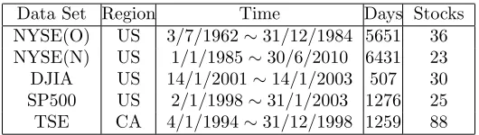
We conduct extensive experiments on 5 benchmark data sets from real-world stock markets: NYSE(O) (Cover, 1991), NYSE(N) (Li et al., 2013), DJIA (Borodin et al., 2004), SP500 (Borodin et al., 2004), and TSE (Borodin et al., 2004). They consist of daily price relatives from New York Stock Exchange, Dow Jones Industrial Average, Standard & Pool 500 and Toronto Stock Exchange, covering a wide range of assets and time spans. Their information is shown in Table 2. To be consistent across the experiments, all the involved returns and increasing factors in this section are daily but not annualized.
We also show the box plots of asset price relatives on the 5 benchmark data sets in Figure
2. Note that if Assetidoes not change in price at day (period)t, thenx(ti) = p
(i)
t
p(ti−1)
= 1, which
Data Set Region Time Days Stocks NYSE(O) US 3/7/1962∼31/12/1984 5651 36 NYSE(N) US 1/1/1985∼30/6/2010 6431 23 DJIA US 14/1/2001∼14/1/2003 507 30 SP500 US 2/1/1998∼31/1/2003 1276 25 TSE CA 4/1/1994∼31/12/1998 1259 88
Table 2: Information of 5 benchmark data sets from real-world stock markets.
they are reliable to test the performance of different PO systems in real-world financial environments.
For comparison, 7 state-of-the-art short-term PO systems are evaluated: ONS (Agarwal et al., 2006), CORN, Anticor, PAMR (Li et al., 2012), CWMR (Li et al., 2013), OLMAR and RMR, as well as 2 trivial ones: Beststock and Market. The parameters for these systems are set by the defaults in their original papers and previous experiments (Li and Hoi, 2014; Li et al., 2016, 2015; Huang et al., 2016): ONS: η = 0, β = 1, γ = 18; CORN: w = 5, P = 1, ρ = 0.1; Anticor: w = 5; PAMR and CWMR: = 0.5; OLMAR: w = 5, = 10; RMR:
w= 5, = 5. The parameters for SSPO are set as: w= 5, λ= 0.5, γ= 0.01, η= 0.005, ζ = 500. Note that the window sizew= 5 is the same with all these systems, to be consistent. Evaluation protocols mainly fall into 8 indicators: 1. Cumulative wealth (CW): the main score to evaluate investing performance; 2. Mean Excess Return (MER) (Jegadeesh, 1990): the average excess performance of a system compared with the market; 3. α Factor (Lintner, 1965): MER excluding the market risk; 4. Order statistics: the rank of a system return in all the asset returns; 5. Sharpe Ratio (Sharpe, 1966): risk-adjusted average return; 6. Information Ratio (Treynor and Black, 1973): risk-adjusted MER; 7. Transaction costs; 8. Running times. Indicators 1∼3 are investing performance measurements, Indicators 4∼6 are risk metrics, and Indicators 7,8 evaluate the applicability to real-world financial environments. SSPO achieves state-of-the-art results in all these indicators.
4.1. Parameter Setting
We first conduct experiments of the final cumulative wealth (CW) to empirically set the parameters for SSPO, which is similar to Borodin et al. (2004); Li et al. (2011, 2015); Huang et al. (2013, 2016). The final CW is the cumulative product of the actual increasing factors{bˆ>t xt}nt=1 with the initial wealthS0 = 1.
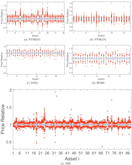
First, w= 5 is a common window size in real-world stock trading, especially in short-term investment. It is also consistent with the compared state-of-the-art methods. Hence it is adopted for SSPO. Second, we fixw= 5,γ = 0.01,η= 0.005,ζ = 500 and changeλin 0.4∼0.65. The results in Figure 3 show thatλ= 0.5 leads to good performance in general and thus is set for SSPO. To better show the geometric scaling effect of the daily geometric increasing factor on the final CW, the power form is used to label the y-axis. The base is the daily geometric increasing factor while the exponent is the total number of trading days in the data set.
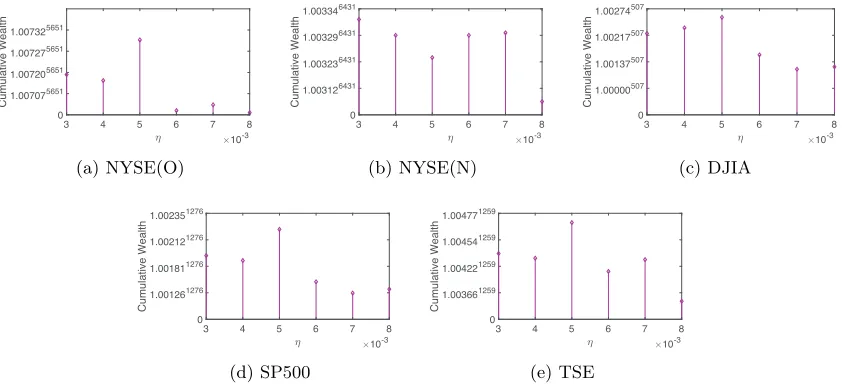
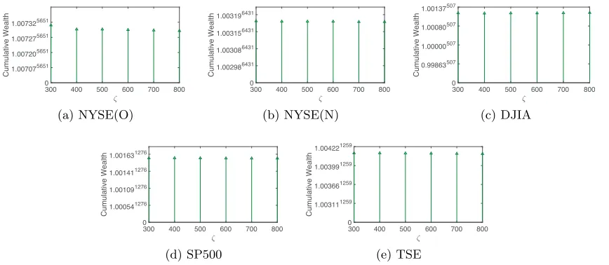
At each time, we change one parameter and fix other parameters, and the results are shown in Figure 4, Figure 5, and Figure 6. They indicate that γ = 0.01, η = 0.005, and
1 6 11 16 21 26 31 36 Asset i
0.8 0.9 1 1.1 1.2 1.3
Pri
ce
R
e
la
ti
ve
(a) NYSE(O)
1 6 11 16 21
Asset i 0.4
0.6 0.8 1 1.2 1.4 1.6 1.8
Pri
ce
R
e
la
ti
ve
(b) NYSE(N)
1 6 11 16 21 26
Asset i 0.4
0.6 0.8 1 1.2
Pri
ce
R
e
la
ti
ve
(c) DJIA
1 6 11 16 21
Asset i
0.7 0.8 0.9 1 1.1 1.2
Pri
ce
R
e
la
ti
ve
(d) SP500
1
6
11 16 21 26 31 36 41 46 51 56 61 66 71 76 81 86
Asset i
0.5
1
1.5
2
Pri
ce
R
e
la
ti
ve
(e) TSE
0 1.007075651 1.007205651 1.007275651 1.007325651 C u mu la ti ve W e a lt h
0.4 0.45 0.5 0.55 0.6 0.65
(a) NYSE(O) 0 1.003126431 1.003236431 1.003296431 1.003346431 C u mu la ti ve W e a lt h
0.4 0.45 0.5 0.55 0.6 0.65
(b) NYSE(N) 0 0.99863507 1.00000507 1.00080507 1.00137507 C u mu la ti ve W e a lt h
0.4 0.45 0.5 0.55 0.6 0.65
(c) DJIA 0 1.000541276 1.001091276 1.001411276 1.001631276 C u mu la ti ve W e a lt h
0.4 0.45 0.5 0.55 0.6 0.65
(d) SP500 0 1.003111259 1.003661259 1.003991259 1.004221259 C u mu la ti ve W e a lt h
0.4 0.45 0.5 0.55 0.6 0.65
(e) TSE
Figure 3: Final cumulative wealths of SSPO with respect to λ on 5 benchmark data sets (fix w= 5, γ = 0.01, η = 0.005, ζ = 500). The power form is used to label the y-axis to better show the geometric scaling effect of the daily geometric increasing factor on the final cumulative wealth. The base is the daily geometric increasing factor while the exponent is the total number of trading days in the data set.
0 1.007075651 1.007205651 1.007275651 1.007325651 C u mu la ti ve W e a lt h
3 4 5 6 7 8
10-3 (a) NYSE(O) 0 1.003126431 1.003236431 1.003296431 1.003346431 C u mu la ti ve W e a lt h
3 4 5 6 7 8
10-3 (b) NYSE(N) 0 1.00000507 1.00137507 1.00217507 1.00274507 C u mu la ti ve W e a lt h
3 4 5 6 7 8
10-3 (c) DJIA 0 1.001261276 1.001811276 1.002121276 1.002351276 C u mu la ti ve W e a lt h
3 4 5 6 7 8
10-3 (d) SP500 0 1.003661259 1.004221259 1.004541259 1.004771259 C u mu la ti ve W e a lt h
3 4 5 6 7 8
10-3
(e) TSE
Figure 4: Final cumulative wealths of SSPO with respect to η on 5 benchmark data sets (fixw= 5,γ = 0.01, λ= 0.5,ζ = 500).
4.2. Cumulative Wealth
0 1.007075651 1.007205651 1.007275651 1.007325651 C u mu la ti ve W e a lt h
0.008 0.009 0.01 0.011 0.012 0.013
(a) NYSE(O) 0 1.003236431 1.003346431 1.003406431 1.003446431 C u mu la ti ve W e a lt h
0.008 0.009 0.01 0.011 0.012 0.013
(b) NYSE(N) 0 1.00000507 1.00137507 1.00217507 1.00274507 C u mu la ti ve W e a lt h
0.008 0.009 0.01 0.011 0.012 0.013
(c) DJIA 0 1.001261276 1.001811276 1.002121276 1.002351276 C u mu la ti ve W e a lt h
0.008 0.009 0.01 0.011 0.012 0.013
(d) SP500 0 1.003661259 1.004221259 1.004541259 1.004771259 C u mu la ti ve W e a lt h
0.008 0.009 0.01 0.011 0.012 0.013
(e) TSE
Figure 5: Final cumulative wealths of SSPO with respect to γ on 5 benchmark data sets (fixw= 5,η = 0.005,λ= 0.5,ζ = 500).
0 1.007075651 1.007205651 1.007275651 1.007325651 C u mu la ti ve W e a lt h
300 400 500 600 700 800
(a) NYSE(O) 0 1.002986431 1.003086431 1.003156431 1.003196431 C u mu la ti ve W e a lt h
300 400 500 600 700 800
(b) NYSE(N) 0 0.99863507 1.00000507 1.00080507 1.00137507 C u mu la ti ve W e a lt h
300 400 500 600 700 800
(c) DJIA 0 1.000541276 1.001091276 1.001411276 1.001631276 C u mu la ti ve W e a lt h
300 400 500 600 700 800
(d) SP500 0 1.003111259 1.003661259 1.003991259 1.004221259 C u mu la ti ve W e a lt h
300 400 500 600 700 800
(e) TSE
Figure 6: Final cumulative wealths of SSPO with respect to ζ on 5 benchmark data sets (fixw= 5,η = 0.005,λ= 0.5,γ = 0.01).
which are much higher than OLMAR (7.21E+16, 4.14E+8 and 58.51) and RMR (1.64E+17, 3.25E+8 and 181.34). Therefore, SSPO is an efficient short-term PO system for diverse real-world stock markets. We also plot the CW evolution paths for different PO systems on DJIA in Figure 7. On most days, the SSPO plot is over other systems, and it climbs up significantly when there are good opportunities.
NYSE(O) NYSE(N) DJIA SP500 TSE
Market 14.50≈1.000475651 18.06≈1.000456431 0.76≈0.99947507 1.34≈1.000231276 1.61≈1.000381259
Beststock 54.14≈1.000715651 83.51≈1.000696431 1.19≈1.00034507 3.78≈1.001041276 6.28≈1.001461259
ONS 109.19≈1.000835651 21.59≈1.000486431 1.53≈1.00084507 3.34≈1.000951276 1.62≈1.000381259
CORN 8.09E+11≈1.004865651 2.33E+5≈1.001926431 0.78≈0.99951507 5.29≈1.001311276 9.80≈1.0001811259
Anticor 2.04E+7≈1.002985651 2.11E+5≈1.001916431 1.63≈1.00096507 5.61≈1.001351276 28.68≈1.002671259
PAMR 5.14E+15≈1.006425651 1.25E+6≈1.002196431 0.68≈0.99924507 5.09≈1.001281276 264.86≈1.004441259
CWMR 6.49E+15≈1.006465651 1.41E+6≈1.002206431 0.69≈0.99926507 5.95≈1.001401276 332.62≈1.004621259
OLMAR 7.21E+16≈1.006895651 4.14E+8≈1.003096431 2.54≈1.00184507 15.94≈1.002171276 58.51≈1.003241259
RMR 1.64E+17≈1.007045651 3.25E+8≈1.003056431 2.67≈1.00194507 8.28≈1.001661276 181.34≈1.004141259
SSPO 1.06E+18≈1.007375651 1.62E+9≈1.003306431 3.68≈1.00257507 16.97≈1.002221276 364.94≈1.004701259
Table 3: Final cumulative wealths of portfolio optimization systems on 5 benchmark data sets. The approximate power form is used to make an intuitive sense of the ge-ometric scaling effect of the daily gege-ometric increasing factor on the final CW. The base is the daily geometric increasing factor while the exponent is the total number of trading days in the data set.
100 200 300 400 500
Period
1.00000507
1.00080507
1.00137507
C
u
mu
la
ti
ve
W
e
a
lt
h
SSPO RMR OLMAR
CWMR PAMR Anticor CORN ONS
Beststock Market
Figure 7: Cumulative wealth evolution paths of portfolio optimization systems on DJIA. The length of one period is one day.
4.3. Mean Excess Return
Mean Excess Return (MER) (Jegadeesh, 1990) is the average daily excess return of a system compared with the market in the long run:
M ER= ¯rs−¯rm =
1
n
n
X
t=1
(rs,t−rm,t), (35)
where rs,t and rm,t are daily returns of a PO system and the market on the t-th day,
respectively. It is more worthy of implementing a PO system with a higher MER. Even a small difference of MER leads to a large gap of CW in the long run, due to the geometric scaling effect.
We present the MERs for different PO systems in Table 4. SSPO outperforms other state-of-the-art systems on all the data sets. For instance, the MERs of SSPO (0.0036 and 0.0060) are much higher than those of OLMAR (0.0028 and 0.0045) and RMR (0.0029 and 0.0053) on DJIA and TSE, respectively. This is the reason why SSPO outperforms other systems in cumulative wealth in the long run.
System NYSE(O) NYSE(N) DJIA SP500 TSE Beststock 0.0003 0.0003 0.0011 0.0012 0.0016
ONS 0.0004 0.0003 0.0015 0.0007 0.0002 CORN 0.0049 0.0017 0.0002 0.0014 0.0020 Anticor 0.0026 0.0016 0.0016 0.0013 0.0027 PAMR 0.0064 0.0021 0.0001 0.0014 0.0050 CWMR 0.0064 0.0022 0.0001 0.0015 0.0053 OLMAR 0.0070 0.0032 0.0028 0.0024 0.0045 RMR 0.0071 0.0032 0.0029 0.0019 0.0053
SSPO 0.0076 0.0035 0.0036 0.0025 0.0060
Table 4: Mean excess returns of portfolio optimization systems on 5 benchmark data sets.
4.4. α Factor
According to the Capital Asset Pricing Model (CAPM) (Sharpe, 1964), the expected return of a system can be decomposed into 2 parts: the market return component, and the intrinsic excess return usually called the α Factor in the finance industry (Lintner, 1965). The former is determined by the market environment, which cannot be improved by any active investing strategy or PO system, while the latter can be improved by a good PO system. Theα Factor can be represented as follows:
E(rs) = βE(rm) +α, (36)
ˆ
β = ˆc(rs, rm) ˆ
σ2(r
m)
, αˆ = ¯rs−βˆr¯m, (37)
whereE(·) denotes the mathematical expectation, ˆc(·,·) and ˆσ(·) are the sample covariance and the sample standard deviation (STD) computed on n trading days, respectively. In finance, STD is a common tool to measure risk (volatility).
In the real-world portfolio management, it is common to perform a right-tailed t-test to see whether α is significantly >0. If so, it indicates that the good performance of the system is not due to luck (Grinold and Kahn, 1999; Li et al., 2015; Huang et al., 2013, 2016). According to the results in Table 5, SSPO achieves significantly better performance than the market at a high confidence level of 99% (with all p-values<0.01).
System NYSE(O) NYSE(N) DJIA SP500 TSE
α p-Value α p-Value α p-Value α p-Value α p-Value
Beststock 0.0003 0.0195 0.0004 0.0176 0.0012 0.0838 0.0011 0.0593 0.0014 0.0606
ONS 0.0005 <0.0001 0.0003 0.1257 0.0016 <0.0001 0.0008 0.0040 0.0002 0.3514
CORN 0.0048 <0.0001 0.0016 <0.0001 0.0002 0.4077 0.0013 0.0190 0.0018 0.0278
Anticor 0.0026 <0.0001 0.0016 <0.0001 0.0017 0.0010 0.0012 0.0021 0.0025 <0.0001
PAMR 0.0063 <0.0001 0.0021 <0.0001 0.0002 0.4275 0.0013 0.0259 0.0048 <0.0001
CWMR 0.0063 <0.0001 0.0021 <0.0001 0.0002 0.4168 0.0014 0.0170 0.0051 <0.0001
OLMAR 0.0069 <0.0001 0.0031 <0.0001 0.0029 0.0065 0.0023 0.0017 0.0042 0.0050
RMR 0.0070 <0.0001 0.0031 <0.0001 0.0030 0.0054 0.0018 0.0102 0.0051 <0.0001
SSPO 0.0074 <0.0001 0.0034 <0.0001 0.0037 0.0009 0.0024 0.0019 0.0058 <0.0001
Table 5: α factors (with p-values of t-tests) of portfolio optimization systems on 5 bench-mark data sets.
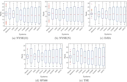
4.5. Order Statistics
One may worry about that a PO system just simply selects the lucky assets with the highest growth. To check this point, we can compare the system return rs,t = ˆb>t xt−1
with all the asset returns r(ti) =xt(i)−1,i= 1,· · · , d(dis the number of assets in a data set). By sorting the (d+ 1) returns{rs,t}S{rt(i)}di=1 in the descending order, we can obtain
the rank of rs,t. If a PO system always chooses the lucky assets, thenrs,t will always rank
very high in the investment.
We give a summary description of the rank of rs,t in the whole investment (n days)
Marke t
Best stock ON
S CO
RN Ant
icor PAMRCW
MR OLM
AR RMRSSPO
Systems 0 5 10 15 20 25 30 35 R a n k (a) NYSE(O) Marke t Best stock ON
S CO
RN Ant
icor PAMRCW
MR OLM
AR RMR SSPO Systems 0 5 10 15 20 25 R a n k (b) NYSE(N) Ma rket Best stock ON
S CO RN Ant icor PA MR CW MR OLM
AR RMR SSPO Systems 0 5 10 15 20 25 30 R a n k (c) DJIA Marke t Best stock ON
S CO
RN Ant
icor PAMRCW
MR OLM
AR RMRSSPO
Systems 0 5 10 15 20 25 R a n k (d) SP500 Marke t Best stock ON
S CO
RN Ant
icor PAMRCW
MR OLM
AR RMR SSPO Systems 0 20 40 60 80 R a n k (e) TSE
Figure 8: Box plots of the ranks for the system returnsrs,t on 5 benchmark data sets. The
ranks for SSPO cover a wide range instead of concentrating on the highest ranks.
System NYSE(O): 37 NYSE(N): 24 DJIA: 31 SP500: 26 TSE: 89 Median Mean Median Mean Median Mean Median Mean Median Mean Market 19 18.63 12 12.25 16 16.12 13 13.34 43 42.88 Beststock 19 19.34 13 12.76 16 16.32 14 14.05 52 47.09 ONS 19 18.56 12 12.42 15 15.35 13 13.01 45 44.83 CORN 18 18.08 12 12.10 16 16.04 13 13.26 46 44.87 Anticor 17 17.25 12 11.72 15 15.32 13 12.98 39 41.77 PAMR 16 17.27 12 12.22 15 16.05 13 13.22 35 40.11 CWMR 16 17.22 12 12.19 16 16.09 13 13.18 35 40.01 OLMAR 17 17.56 12 12.26 15 15.45 12 13.31 43 43.12 RMR 16 17.40 12 12.26 15 15.34 13 13.40 40 42.18
SSPO 17 17.71 12 12.25 15 15.25 12 13.33 44 43.03
Table 6: Medians and means of the ranks for the system returnsrs,t on 5 benchmark data
4.6. Sharpe Ratio
In general, when an investor pursues high return, he/she should be ready to undertake high risk. Thus he/she has to balance between return and risk all the time. Sharpe Ratio (SR) (Sharpe, 1966) is such a measurement to meet this demand based on CAPM:
SR= ¯rs−rf ˆ
σ(rs)
, (38)
where rf is the daily return of some risk-free asset, which is not considered in this paper.
Hence we setrf = 0 to make SR a daily risk-adjusted return.
We compute and present the daily SRs of different PO systems in Table 7. SSPO achieves the highest SR on NYSE(N) and DJIA, and is close to the best system on other data sets. Besides, SSPO is competitive to OLMAR and RMR. For example, SSPO achieves
SR = 0.0791 on SP500 compared with RMR (0.0659), and achieves SR= 0.1054 on TSE compared with OLMAR (0.0820). It indicates that SSPO has a good ability in balancing between return and risk on the premise of good investing achievement with high CWs.
System NYSE(O) NYSE(N) DJIA SP500 TSE
SR IR SR IR SR IR SR IR SR IR
Market 0.0549 Null 0.0458 Null −0.0273 Null 0.0224 Null 0.0491 Null
Beststock 0.0536 0.0241 0.0472 0.0225 0.0253 0.0560 0.0485 0.0468 0.0579 0.0490
ONS 0.0789 0.0424 0.0313 0.0129 0.0504 0.1574 0.0701 0.0582 0.0281 0.0093
CORN 0.1635 0.1570 0.0968 0.0859 −0.0097 0.0108 0.0581 0.0618 0.0675 0.0595
Anticor 0.1720 0.1743 0.0973 0.0899 0.0535 0.1255 0.0682 0.0834 0.1061 0.0993
PAMR 0.2149 0.2121 0.0864 0.0763 −0.0115 0.0036 0.0568 0.0573 0.1182 0.1131
CWMR 0.2169 0.2143 0.0858 0.0758 −0.0106 0.0047 0.0606 0.0623 0.1179 0.1129
OLMAR 0.2102 0.2071 0.1038 0.0958 0.0731 0.1058 0.0806 0.0848 0.0820 0.0769
RMR 0.2153 0.2123 0.1033 0.0953 0.0763 0.1092 0.0659 0.0678 0.0981 0.0932
SSPO 0.2073 0.2041 0.1060 0.0979 0.0919 0.1304 0.0791 0.0840 0.1054 0.1009
Table 7: Daily Sharpe Ratios (SR) and daily Information Ratios (IR) of portfolio optimiza-tion systems on 5 benchmark data sets.
4.7. Information Ratio
Different from SR, Information Ratio (IR) (Treynor and Black, 1973) directly measures the daily risk-adjusted excess return of a system compared with the market, which can be seen as a combination of MER and SR. It is also worth reference for the concern with risk.
IR= (¯rs−¯rm) ˆ
σ(rs−rm)
. (39)
4.8. Transaction Costs
In practice, transaction cost is an important issue in PO. Suppose we have to pay at a transaction cost rateν∈(0,1) to update the portfolio. Then according to the proportional transaction cost model (Blum and Kalai, 1999; Li et al., 2015; Huang et al., 2016), the cumulative wealth at the beginning of thet-th day is
Snν = S0
n
Y
t=1
[(ˆb>txt)·(1−
ν
2
d
X
i=1
|bˆ(ti)−b˜t(−i)1|)], (40)
˜
b(ti−)1 = ˆ
b(ti−)1·x(ti−)1 ˆ
b>t−1xt−1
, (41)
where ˜b(ti−)1 denotes the adjusted portfolio of Asset iat the end of the (t−1)-th day and ˜
b0 is set as [0,· · ·,0]>. ν2Pdi=1|bˆ (i)
t −b˜
(i)
t−1| is the proportional transaction cost when we
change the adjusted portfolio ˜bt−1 to the next portfolio ˆbt.
To test the effectiveness of SSPO with consideration of transaction cost, we conduct experiments of cumulative wealth withν= 0∼0.5%, whereν = 0.5% is a rather high cost rate for stock transactions. The results shown in Figure 9 indicate that SSPO outperforms the two state-of-the-art systems OLMAR and RMR on all the data sets and thus it is applicable to real-world financial environments.
0 0.1 0.2 0.3 0.4 0.5
Transaction Cost Rate (%)
105 1010 1015 1020 C u mu la ti ve W e a lt h SSPO OLMAR RMR (a) NYSE(O)
0 0.1 0.2 0.3 0.4 0.5 Transaction Cost Rate (%) 10-5 100 105 1010 C u mu la ti ve W e a lt h SSPO OLMAR RMR (b) NYSE(N)
0 0.1 0.2 0.3 0.4 0.5
Transaction Cost Rate (%)
0 0.5 1 1.5 2 2.5 3 3.5 4 C u mu la ti ve W e a lt h SSPO OLMAR RMR (c) DJIA
0 0.1 0.2 0.3 0.4 0.5
Transaction Cost Rate (%)
0 5 10 15 20 C u mu la ti ve W e a lt h SSPO OLMAR RMR (d) SP500
0 0.1 0.2 0.3 0.4 0.5
Transaction Cost Rate (%)
0 50 100 150 200 250 300 350 400 C u mu la ti ve W e a lt h SSPO OLMAR RMR (e) TSE
4.9. Running Times
We use a computer with an AMD A10-7800 CPU and an 8GB DDR3 1600MHz memory card to run SSPO in the experiments, which shows that it is sufficiently fast for large-scale and time-limited trading environments such as High-Frequency Trading (HFT) (Aldridge, 2013). The average running times (in seconds) of SSPO for one trade on different data sets are: NYSE(O) (0.0576s), NYSE(N) (0.0450s), DJIA (0.0455s), SP500 (0.0449s), and TSE (0.1190s). Hence SSPO has good computational efficiency besides significant investing advantage.
5. Conclusions
We present a novel short-term sparse portfolio optimization (SSPO) system to concen-trate wealth on a few assets with good increasing potential according to some empirical financial principles. Few short-term PO systems construct sparse portfolios, and most ex-isting sparsity systems are either lazy updates or for the long-term PO. These problems motivate the design of SSPO. We further propose an ADMM algorithm for SSPO, and prove that its augmented Lagrangian has a saddle point. This is the foundation of the iterative formulae of ADMM but is seldom addressed before.
We conduct extensive experiments on 5 benchmark data sets with diverse real-world stock data, which shows that SSPO outperforms other state-of-the-art short-term PO sys-tems with all the investing performance measurements (cumulative wealth, mean excess return and α Factor) on all the benchmark data sets. The order statistics of the SSPO returns also indicate that SSPO does not simply select the lucky assets with the highest growth and its returns are credible. SSPO is also competitive to other systems on the risk metrics SR and IR, and shows robustness in balancing between return and risk. Further-more, SSPO can withstand reasonable transaction costs and runs fast, thus it is applicable to real-world financial environments including High-Frequency Trading. Therefore, SSPO is an effective and robust system that is worth further investigations. In the future, we will continue to establish more complex SSPO systems, so as to improve the investing performance and the robustness to risk.
Acknowledgments
References
A. Agarwal, E. Hazan, S. Kale, and R. E. Schapire. Algorithms for portfolio management based on the Newton method. InProceedings of the International Conference on Machine
Learning (ICML), 2006.
I. Aldridge. High-Frequency Trading: A Practical Guide to Algorithmic Strategies and
Trading Systems. Wiley, Hoboken, NJ, 2 edition, Apr. 2013.
D. Bertsekas. Nonlinear Programming. Athena Scientific, 1999.
A. Blum and A. Kalai. Universal portfolios with and without transaction costs. Machine
Learning, 35(3):193–205, 1999.
W. F. M. D. Bondt and R. Thaler. Does the stock market overreact? Journal of Finance, 40(3):793–805, Jul. 1985.
A. Borodin, R. El-Yaniv, and V. Gogan. Can we learn to beat the best stock. Journal of
Artificial Intelligence Research, 21(1):579–594, Jan. 2004.
S. Boyd and L. Vandenberghe. Convex Optimization. Cambridge University Press, 2004.
S. Boyd, N. Parikh, E. Chu, B. Peleato, and J. Eckstein. Distributed optimization and statistical learning via the alternating direction method of multipliers. Foundations and
Trends in Machine Learning, 3(1):1–122, 2010.
J. Brodie, I. Daubechies, C. D. Giannone, and I. Loris. Sparse and stable Markowitz port-folios. Proceedings of the National Academy of Sciences of the United States of America, 106(30):12267–12272, Jul. 2009.
E. J. Cand`es and Y. Plan. Near-ideal model selection by `1 minimization. Annals of
Statistics, 37(5A):2145–2177, 2009.
T. M. Cover. Universal portfolios. Mathematical Finance, 1(1):1–29, Jan. 1991.
P. Das, N. Johnson, and A. Banerjee. Online lazy updates for portfolio selection with trans-action costs. In Proceedings of the AAAI Conference on Artificial Intelligence (AAAI), pages 202–208, 2013.
J. Duchi, S. Shalev-Shwartz, Y. Singer, and T. Chandra. Efficient projections onto the
`1-ball for learning in high dimensions. InProceedings of the International Conference on
Machine Learning (ICML), 2008.
E. F. Fama. The behavior of stock-market prices. Journal of Business, 38(1):34–105, Jan. 1965.
E. F. Fama. Efficient capital markets: A review of theory and empirical work. Journal of
Finance, 25(2):383–417, May 1970.
R. Fernholz. Stochastic Portfolio Theory. Springer Verlag, 2002.
R. Grinold and R. Kahn. Active Portfolio Management: A Quantitative Approach for
Producing Superior Returns and Controlling Risk. McGraw-Hill, New York, 1999.
L. Gy¨orfi, G. Lugosi, and F. Udina. Nonparametric kernel-based sequential investment strategies. Mathematical Finance, 16(2):337–357, Apr. 2006.
J. He, Q. G. Wang, P. Cheng, J. Chen, and Y. Sun. Multi-period mean-variance portfolio optimization with high-order coupled asset dynamics. IEEE Transactions on Automatic
Control, 60(5):1320–1335, May 2015.
M. Ho, Z. Sun, and J. Xin. Weighted elastic net penalized mean-variance portfolio design and computation. SIAM Journal on Financial Mathematics, 6(1), 2015.
D. Huang, J. Zhou, B. Li, S. C. H. Hoi, and S. Zhou. Robust median reversion strategy for on-line portfolio selection. In Proceeding of the International Joint Conference on
Artificial Intelligence (IJCAI), pages 2006–2012, 2013.
D. Huang, J. Zhou, B. Li, S. C. H. Hoi, and S. Zhou. Robust median reversion strategy for online portfolio selection. IEEE Transactions on Knowledge and Data Engineering, 28 (9):2480–2493, Sep. 2016.
N. Jegadeesh. Evidence of predictable behavior of security returns. Journal of Finance, 45 (3):881–898, Jul. 1990.
N. Jegadeesh. Seasonality in stock price mean reversion: Evidence from the U.S. and the
U.K. Journal of Finance, 46(4):1427–1444, Sep. 1991.
N. Jegadeesh and S. Titman. Returns to buying winners and selling losers: Implications for stock market efficiency. Journal of Finance, 48(1):65–91, Mar. 1993.
D. Kahneman and A. Tversky. Prospect theory: An analysis of decision under risk.
Econo-metrica, 47(2):263–292, Mar. 1979.
Z. R. Lai, D. Q. Dai, C. X. Ren, and K. K. Huang. Discriminative and compact coding for robust face recognition. IEEE Transactions on Cybernetics, 45(9):1900–1912, Sep. 2015.
B. Li and S. C. H. Hoi. On-line portfolio selection with moving average reversion. In
Proceedings of the International Conference on Machine Learning (ICML), 2012.
B. Li and S. C. H. Hoi. Online portfolio selection: A survey. ACM Computing Surveys
(CSUR), 46(3):35:1–35:36, 2014.
B. Li, S. C. H. Hoi, and V. Gopalkrishnan. CORN: Correlation-driven nonparametric learning approach for portfolio selection. ACM Transactions on Intelligent Systems and
Technology, 2(3), Apr. 2011. Article No.21.
B. Li, S. C. H. Hoi, P. Zhao, and V. Gopalkrishnan. Confidence weighted mean reversion strategy for online portfolio selection. ACM Transactions on Knowledge Discovery from Data, 7(1), Mar. 2013. Article 4.
B. Li, S. C. H. Hoi, D. Sahoo, and Z. Y. Liu. Moving average reversion strategy for on-line portfolio selection. Artificial Intelligence, 222:104–123, 2015.
B. Li, D. Sahoo, and S. C. H. Hoi. OLPS: a toolbox for on-line portfolio selection. Journal
of Machine Learning Research, 17(1):1242–1246, 2016.
J. Lintner. The valuation of risk assets and the selection of risky investments in stock portfolios and capital budgets. Review of Economics and Statistics, 47(1):13–37, Feb. 1965.
B. Mahdavi-Damghani, K. Mustafayeva, S. Roberts, and C. Buescu. Portfolio optimization in the context of cointelated pairs: Stochastic differential equation vs. machine learning approach. Social Science Electronic Publishing, 2017.
S. Maillard, T. Roncalli, and J. Teiletche. On the properties of equally-weighted risk con-tributions portfolios. Social Science Electronic Publishing, 36(4):60–70, 2010.
H. M. Markowitz. Portfolio selection. Journal of Finance, 7(1):77–91, Mar. 1952.
Y. Q. Mohsin, G. Ongie, and M. Jacob. Iterative shrinkage algorithm for patch-smoothness regularized medical image recovery. IEEE Transactions on Medical Imaging, 34(12): 2417–2428, Dec. 2015.
W. F. Sharpe. Capital asset prices: A theory of market equilibrium under conditions of risk. Journal of Finance, 19(3):425–442, Sep. 1964.
W. F. Sharpe. Mutual fund performance. Journal of Business, 39(1):119–138, Jan. 1966.
W. Shen, J. Wang, and S. Ma. Doubly regularized portfolio with risk minimization. In
Proceedings of the AAAI Conference on Artificial Intelligence (AAAI), 2014.
R. J. Shiller. Irrational Exuberance. Princeton University Press, Princeton, NJ, 2000.
R. J. Shiller. From efficient markets theory to behavioral finance. Journal of Economic
Perspectives, 17(1):83–104, 2003.
S. Still and I. Kondor. Regularizing portfolio optimization. New Journal of Physics, 12: 1–14, 2010.
R. Tibshirani. Regression shrinkage and selection via the lasso. Journal of the Royal
Statistical Society, 58(1):267–288, 1996.
J. L. Treynor and F. Black. How to use security analysis to improve portfolio selection.
Journal of Business, 46(1):66–86, Jan. 1973.
Y. Vardi and C. H. Zhang. The multivariate `1-median and associated data depth.
Pro-ceedings of the National Academy of Sciences of the United States of America, 97(4):
L. Yang, R. Couillet, and M. R. McKay. A robust statistics approach to minimum variance portfolio optimization. IEEE Transactions on Signal Processing, 63(24):6684–6697, Dec. 2015.
P. Yin, Y. Lou, Q. He, and J. Xin. Minimization of `1−2 for compressed sensing. SIAM
Journal on Scientific Computing, 37(1):A536–A563, 2015.
Z. Zhan, J. F. Cai, D. Guo, Y. Liu, Z. Chen, and X. Qu. Fast multiclass dictionaries learning with geometrical directions in MRI reconstruction. IEEE Transactions on Biomedical
Engineering, 63(9):1850–1861, Sep. 2016.
H. Zou and T. Hastie. Regularization and variable selection via the elastic net. Journal of