Extrapolating Expected Accuracies for Large Multi-Class
Problems
Charles Zheng [email protected]
Section on Functional Imaging Methods National Institute of Mental Health Bethesda, MD
Rakesh Achanta [email protected]
Department of Statistics Stanford University Palo Alto, CA
Yuval Benjamini [email protected]
Department of Statistics
The Hebrew University of Jerusalem, Jerusalem, Israel
Editor:Christoph Lampert
Abstract
The difficulty of multi-class classification generally increases with the number of classes. Using data for a small set of the classes, can we predict how well the classifier scales as the number of classes increases? We propose a framework for studying this question, assuming that classes in both sets are sampled from the same population and that the classifier is based on independently learned scoring functions. Under this framework, we can express the classification accuracy on a set ofkclasses as the (k−1)st moment of a discriminability function; the discriminability function itself does not depend onk. We leverage this result to develop a non-parametric regression estimator for the discriminability function, which can extrapolate accuracy results to larger unobserved sets. We also formalize an alterna-tive approach that extrapolates accuracy separately for each class, and identify tradeoffs between the two methods. We show that both methods can accurately predict classifier performance on label sets up to ten times the size of the original set, both in simulations as well as in realistic face recognition or character recognition tasks.
Keywords: Multi-class problems, face recognition, object recognition, transfer learning, nonparametric models
1. Introduction
Many machine learning tasks are interested in recognizing or identifying an individual in-stance within a large set of possible candidates. These problems are usually modeled as multi-class classification problems, with a large and possibly complex label set. Leading ex-amples include detecting the speaker from his voice patterns (Togneri and Pullella, 2011), identifying the author from her written text (Stamatatos et al., 2014), or labeling the object category from its image (Duygulu et al., 2002; Deng et al., 2010; Oquab et al., 2014). In
c
all these examples, the algorithm observes an inputx, and uses the classifier function hto guess the label y from a large label setS.
There are multiple practical challenges in developing classifiers for large label sets. Col-lecting high quality training data is perhaps the main obstacle, as the costs scale with the number of classes. It can be more affordable to first collect data for a small set of classes, even if the long-term goal is to generalize to a larger set. Furthermore, classifier devel-opment can be accelerated by training first on fewer classes, as each training cycle may require substantially less resources. Indeed, due to interest in how small-set performance generalizes to larger sets, such comparisons can found in the literature (Oquab et al., 2014; Griffin et al., 2007). A natural question is: how does changing the size of the label set affect the classification accuracy?
We consider a pair of classification problems on finite label sets: a source task with label set Sk1 of size k1, and a target task with a larger label set Sk2 of size k2 > k1. For each
label set Sk, one constructs the classification rule h(k) :X → Sk. Supposing that in each task, the test example (X∗, Y∗) has a joint distribution, define the generalization accuracy for label setSk as
GAk = Pr[h(k)(X∗) =Y∗]. (1) The problem ofperformance extrapolation is the following: using data from only the source taskSk1, predict the accuracy for a target task with a larger unobserved label setSk2.
A natural use case for performance extrapolation would be in the deployment of a facial recognition system. Suppose a system was developed in the lab on a database ofk1 individuals. Clients would like to deploy this system on a new larger set ofk2 individuals. Performance extrapolation could allow the lab to predict how well the algorithm will perform on the clients’ problem, accounting for the difference in label set size.
Extrapolation should be possible when the source and target classifications belong to the same problem domain. In many cases, the set of categories S is to some degree a random or arbitrary selection out of a larger, perhaps infinite, set of potential categoriesY. Yet any specific experiment uses a fixed finite set. For example, categories in the classical Caltech-256 image recognition data set (Griffin et al., 2007) were assembled by aggregating keywords proposed by students and then collecting matching images from the web. The arbitrary nature of the label set is even more apparent in biometric applications (face recognition, authorship, fingerprint identification) where the labels correspond to human individuals (Togneri and Pullella, 2011; Stamatatos et al., 2014). In all these cases, the number of the labels used to define a concrete data set is therefore an experimental choice rather than a property of the domain. Despite the arbitrary nature of these choices, such data sets are viewed as representing the larger problem of recognition within the given domain, in the sense that success on such a data set should inform performance on similar problems.
In this paper, we assume that both Sk1 and Sk2 are samples consisting of independent and identically distributed (i.i.d.) labels from a population (or prior distribution)π, which is defined on the label spaceY. We have no constraints on the dependence betweenSk1 and
to derive specialized metrics of how similar Sk2 is to Sk1. This simplifies the theory, and demonstrates that in a very general setting, extrapolation is possible. We also make the assumption that the classifiers train a model independently for each class. This convenient property allows us to characterize the accuracy of the classifier by selectively conditioning on one class at a time.
Since we assume the label set is random, the generalization accuracy of a given clas-sifier becomes a random variable. Performance extrapolation then becomes the problem of estimating the average generalization accuracy AGAk of an i.i.d. label set Sk of sizek. Roughly speaking, the achievable accuracy of a classification problem depends on how well the labels can be ‘separated’ based on the training data– that is, how different the empirical distributions of the training data look at the points where new test instances are drawn. The condition of i.i.d. sampling of labels ensures that the separation of labels in a random set Sk2 can be inferred by looking at the empirical separation in Sk1, and therefore that some estimate of the average accuracy on Sk2 can be obtained.
Our paper presents several main contributions related to extrapolation within this frame-work. First, we present a theoretical formula describing how average accuracy for smaller
k is linked to average accuracy for label set of size K > k. We show that accuracy at any size depends on a discriminability function D, which is determined by properties of the data distribution and the classifier but does not depend on k. Second, we propose an estimation procedure that allows extrapolation of the observed average accuracy curve from
k1-class data to a larger number of classes, based on the theoretical formula. Under certain conditions, the estimation method has the property of being an unbiased estimator of the average accuracy. Third, we formalize an alternative approach (proposed by Kay et al. (2008)) that extrapolates accuracy separately for each class, and discuss tradeoffs between the two methods.
The paper is organized as follows. In the rest of this section, we discuss related work. The framework of randomized classification is introduced in Section 2, and there we also introduce a toy example which is revisited throughout the paper. Section 3 develops our theory of extrapolation, and in Section 3.3 we suggest an estimation method. We evaluate our method using simulations in Section 4. In Section 5, we demonstrate our method on a facial recognition problem, as well as an optical character recognition problem. In Section 6 we discuss modeling choices and limitations of our theory, as well as potential extensions.
1.1. Related Work
(2014) presents a method for estimating the accuracy of a classifier which can be used to improve performance for general classifiers, but doesn’t apply for different set sizes.
The theoretical framework we adopt is one where there exists a family of classification problems with increasing number of classes. This framework can be traced back to Shannon (1948), who considered the error rate of a random codebook, which is a special case of randomized classification. More recently, a number of authors have considered the problem of high-dimensional feature selection for multi-class classification with a large number of classes (Pan et al., 2016; Abramovich and Pensky, 2015; Davis et al., 2011). All of these works assume specific distributional models for classification compared to our more general setup. However, we do not deal with the problem of feature selection.
Perhaps the most similar method that deals with extrapolation of classification error to a larger number of classes can be found in Kay et al. (2008). They trained a classifier for identifying the observed stimulus from a functional MRI scan of brain activity, and were interested in its performance on larger stimuli sets. They proposed an extrapolation algorithm, based on per-class kernel density estimation, as a heuristic with little theoretical discussion. In Section 3.5, we formalize their method within our framework, and implement two variations of their algorithm. We present simulation results and theoretical arguments to compare the algorithm to the regression approach we propose.
2. Randomized Classification
The randomized classification model we study has the following features. We assume that there exists an infinite, perhaps continuous, label spaceY and an example spaceX ⊆Rp. In the subsequent theory we assume that Y is continuous solely for the sake of mathematical convenience, so that we can discuss probability integrals on the space without the use of measure-theoretic notation. However, the theory would also approximately describe the case ofY is a sufficiently large discrete space, as long as the probability mass of the largest atom is suitably small.
We assume there exists a prior distribution π on the label space Y, and that for each labely∈ Y, there exists a distribution of examplesFy. In other words, for an example-label pair (X, Y), the conditional distribution ofX givenY =y is given by Fy.
A random classification task can be generated as follows. The label setS ={Y(1), . . . , Y(k)}
is generated by drawing labels Y(1), . . . , Y(k) i.i.d. fromπ. Here we assume the number of labels k to be deterministic. For each label, we sample a training set and a test set. The test set is obtained by sampling r observations X`(i) i.i.d. from FY(i) for` = 1, . . . , r. For
now, we can also assume that the training set is obtained by sampling rtrain observations
X`,train(i) i.i.d. from FY(i) for`= 1, . . . , rtrain and i= 1, . . . , k. However, later we will relax these assumptions on the sampling of the training sets, so that we can accommodate classes have differing or stochastically determined number of instances, as long as the number of training instances for different labels are conditionally independent.
We assume that the classifierh(x) works by assigning a score to each labely(i)∈ S, then choosing the label with the highest score. That is, there exist real-valued score functions my(i)(x) for each label y(i) ∈ S. Here we used the lower-case notation y(i) for the labels,
treating them as fixed for now. Since the classifier is allowed to depend on the training data, it is convenient to view it (and its associated score functions) as random. We write
H(x) when we wish to work with the classifier as a random function, and likewise My(x) to denote the score functions whenever they are considered as random. Since the classifier works by choosing the label with the highest score, the classifier is correct for a given test instancex∗ with true labely∗ whenever my∗(x∗) = maxjm
y(j)(x∗), assuming that there are
no ties.
For a fixed instance of the classification task with labels S = {y(i)}k
i=1 and associ-ated score functions {my(i)}ki=1, recall the definition of the k-class generalization error (1).
We will use the assumption that the test labels are uniformly distributed1 over S, which makes GAk(h,S) abalanced accuracy, which equally weights the accuracies of the individual classes. Assuming that there are no ties, it can be written in terms of score functions as
GAk(h,S) = 1
k
k
X
i=1
Pr[my(i)(X(i)) = max
j my(j)(X (i))],
whereX(i) ∼Fy(i) fori= 1, . . . , k.
However, it is often appropriate to model the labels{Y(i)}k
i=1as a random sample from a distribution. Examples for suchrandomized classification problems include face recognition, where faces are drawn from a larger population, and large multi-class problems where only an arbitrary subset of labels have been collected.
Given our assumption thatkis fixed, a natural target for prediction extrapolation is the expected value of the generalization accuracy GAk(h,S) over the distribution of label sets. We call this the k-class average generalization accuracy of the classifier, denoted AGAk, and formally defined as
AGAk=E[GAk(H,Sk)]
= 1
k
k
X
i=1
Pr[MY(i)(X(i)) = max
j MY(j)(X (i))]
= Pr[MY(X)> k−1 max
j=1 MY(j)(X)]
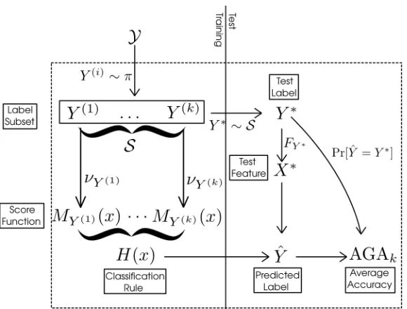
where Y(1), . . . , Y(k) ∼iidπ, and where (X, Y) is an independent draw with the same joint distribution as its superscripted counterparts (X(i), Y(i)). The last line follows from noting that allk summands in the previous line are identical, as eachY(i) is drawn from the same distributionπ. The definition of average generalization accuracy is illustrated in Figure 1.
Note that in this framework, the role of the training and test sets is different than how they are usually used machine learning. Our goal is to predict the accuracy achieved on another (random) label set. Therefore, both the training and test data may be used
Figure 1: Average generalization accuracy: A diagram of the random quantities un-derlying the average generalization accuracy forklabels (AGAk). At the training stage (left), a set ofklabelsSis sampled from the priorπ, and score functions are trained from examples for these classes. At the test stage (right), one true class
Y∗ is sampled uniformly from S, as well as a test example X∗. AGAk measures the expected accuracy over these random variables.
in this estimation. Our approach, to be described in Section 2.3, uses the training data exclusively to construct classifiers on label subsets, and test data exclusively to estimate the distribution of favorability over test examples.
2.1. Marginal Classifier
The theoretical analysis of the average generalization accuracy is made much simpler if we can assume that the learning of the scoring functionsMY(i) occurs independently for each
labels–that is, there is no information shared between classes. For example, if there exists some functiong such that
My(i)(x) =g(x;y(i),(X1(i,train) , ..., Xr(i)
train,train)),
the H is a marginal classifier since My(i)(x) only depends on the label y(i) and the class
training setXj,train(i) .
In our analysis however, we shall relax the assumption that the classifierH(x) is based on a training set2. Instead, it is sufficient that the score functions {MY(i)}ki=1 associated
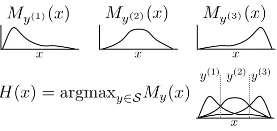
Figure 2: Classification rule: Top: Score functions for three classes in a one-dimensional example space. Bottom: The classification rule chooses betweeny(1), y(2) ory(3)
by choosing the maximal score function.
with the random label set {Y(i)}k
i=1 are independent of the test instances. Under this formalism, we define a marginal classifier as follows.
Definition 1 The classifier H(x) is called a marginal classifier if and only if MY(i) are
independent of both Y(j) and MY(j) for j6=i.
In marginal classifiers, classes “compete” only through selecting the highest score, but not in constructing the score functions. Therefore, each My can be considered to have been independently drawn from a distributionνy. The operation of a marginal classifier is illustrated in Figure 2.
For marginal classifiers, we can prove especially strong results about the accuracy of the classifier under i.i.d. sampling assumptions. And as we will see in the following section, many well-known types of classifiers satisfy the marginal property.
2.2. Examples of Marginal Classifiers
Estimated Bayes classifiers are primary examples of marginal classifiers. By this, we mean classifiers which output the class that maximizes the posterior probability for a class label according to Bayes’ rule, but substituting in estimated distributions for the unknown true distributions. Let ˆfybe a density estimate of the example distribution under labelyobtained from the empirical distribution ˆFy, and letπ(y) be the prior distribution over labels. Then, we can use the estimated density to produce the score functions:
MyEB(x) = log( ˆfy(x)) + log(π(y)).
The resulting empirical approximation for the Bayes classifier would be
HEB(x) = argmaxY∈S(MYEB(x)).
Both Quadratic Discriminant Analysis (QDA) and na¨ıve Bayes classifiers can be seen as specific instances of an estimated Bayes classifier. For QDA, the score function is given by
where µ(F) = R
ydF(y) and Σ(F) = R
(y −µ(F))(y −µ(F))TdF(y). Hence, QDA is the special case of the estimated Bayes classifier when ˆfy is obtained as the multivariate Gaussian density with mean and covariance parameters estimated from the data.
In Na¨ıve Bayes, the score function is
mN By (x) = p
X
j=1
log ˆfy,j(x),
where ˆfy,j is a density estimate for the j-th component of ˆFy. Hence, Na¨ıve Bayes is the estimated Bayes classifier when ˆfy is obtained as the product of estimated componentwise marginal distributions of p(xi|y).
For some classifiers,My is a deterministic function ofy(and thereforeνy is degenerate). A prime example is when there exist fixed or pre-trained embeddings g,˜g that map both labelsy and examplesx intoRp. Then
Myembed=−kg(y)−˜g(x)k2. (2) This would be the case when features from publicly available embeddings (e.g. word em-bedding vectors) are used for classification; see our example in Section 5. See also Pereira et al. (2018) for an example using word embedding vectors. Note that if the embeddings g
or ˜gare informed by the specific set of classes in the experiment, this would no longer be a marginal classifier.
There are many classifiers which do not satisfy the marginal property, such as multino-mial logistic regression, multilayer neural networks, decision trees, and k-nearest neighbors.
2.3. Estimation of Average Accuracy
Before tackling extrapolation, it will be useful for us to discuss the simpler task of generaliz-ing accuracy results when the target set isnot larger than the source set. This allows us to introduce several concepts and notations that are used in the harder problem of generalizing to a larger set. We will also illustrate all of these concept in a toy example following this section, which we shall revisit once more while tackling the problem of extrapolation.
Suppose we have training and test data for a classification task withk1 classes. That is, we have a label setSk1 ={y(i)}k1
i=1, and we assume that the training data has been used to obtain its associated set of score functions My(i). The test set, composed of (x1(i), . . . , x(ri)) for i= 1, . . . , k1 is also available to be used for this estimation task. What would be the predicted accuracy for a new randomly sampled set ofk2≤k1 labels?
Note that AGAk2 is the expected value of the accuracy on the new set of k2 labels.
Therefore, any unbiased estimator of AGAk2 will be an unbiased predictor for the accuracy
on the new set.
Let us start with the case k2=k1 =k. For each test observation x(`i), define the ranks of the candidate classesj = 1, . . . , k by
Ri,j` = k
X
s=1
where we have definedm(`i,j)=my(j)(x
(i)
` ). The test accuracy is the fraction of observations for which the correct class also has the highest rank
TAk= 1 rk k X i=1 r X `=1
I{Ri,i` =k}. (3)
Taking expectations over both the test set and the random labels, the expected value of the test accuracy is AGAk. Therefore, in this special case, TAk provides an unbiased estimator for AGAk2.
Next, let us consider the case wherek2 < k1. Consider label setSk2 obtained by sampling k2 labels uniformly without replacement from Sk1. Since Sk2 is unconditionally an i.i.d.
sample from the population of labels π, the test accuracy of Sk2 is an unbiased estimator of AGAk2. However, we can get a better unbiased estimate of AGAk2 by averaging over all
the possible subsamplesSk2 ⊂ Sk1. This defines the average test accuracy over subsampled
tasks, ATAk2.
Remark. Na¨ıvely, computing ATAk2 requires us to train and evaluate
k1
k2
classification rules. However, for marginal classifiers, retraining the classifier is not necessary. The rank
R`i,iof the correct label iforx(`i), allows us to determine how many subsetsS2 will result in a correct classification. Specifically, there are Ri,i` −1≤k2 labels with a lower score than the correct label i. Therefore, as long as one of the classes inS2 is i, and the other k2−1 labels are from the set of Ri,i` −1 labels with lower score than i, the classification of x(ji)
will be correct. This implies that there are R
i,i ` −1
k2−1
such subsets S2 wherex(`i) is classified correctly, and therefore the average test accuracy for all k1
k2
subsets S2 is
ATAk2 =
1 k1 k2 1 rk2 k1 X i=1 r X `=1
Ri,i` −1
k2−1
. (4)
2.4. Toy Example: Bivariate Normal
Let us illustrate these ideas using a toy example. Let (Y, X) have a bivariate normal joint distribution,
(Y, X)∼N
0 0 , 1 ρ ρ 1 ,
as illustrated in Figure 3(a). Therefore, for a given randomly drawn labelY, the conditional distribution of X for that label is univariate normal with mean ρY and variance 1−ρ2,
X|Y =y∼N(ρy,1−ρ2).
Supposing we drawk= 3 labels{y(1), y(2), y(3)}, the classification problem will be to assign a test instance X∗ to the correct label. The test instance X∗ would be drawn with equal probability from one of three conditional distributions X|Y =y(i), as illustrated in Figure 3(b, top). The Bayes rule assigns X∗ to the class with the highest density p(x|y(i)), as illustrated by Figure 3(b, bottom): it is therefore a marginal classifier, with score function
My(x) = log(p(x|y)) =−
(x−ρy)2
Joint distribution of(X, Y) Problem instance withk= 3
−2 −1 0 1 2
−3
−2
−1
0
1
2
3
rho = 0.7
x
y
E[X|Y=y]
−4 −2 0 2 4
0.0
0.3
0.6
x
density
−4 −2 0 2 4
0.0
0.3
0.6
x
density
(a) (b)
Figure 3: Toy example: Left: The joint distribution of (X, Y) is bivariate normal with correlation ρ = 0.7. Right: A typical classification problem instance from the bivariate normal model withk = 3 classes. (Top): the conditional density ofX
given labelY, forY ={y(1), y(2), y(3)}. (Bottom): the Bayes classification regions for the three classes.
2 4 6 8 10
0.0
0.2
0.4
0.6
0.8
1.0
k
Accur
acy
For this model, the generalization accuracy of the Bayes rule for any label set{y(1), . . . , y(k)}
is given by
GAk(h,{y(1), . . . , y(k)}) = 1
k
k
X
i=1 Pr
X∼p(x|y(i))[p(X|y
(i)) =maxk j=1 p(X|y
(j))]
= 1
k
k
X
i=1 Φ y
[i+1]−y[i] 2p1−ρ2
!
−Φ y
[i−1]−y[i] 2p1−ρ2
!
,
where Φ is the standard normal cdf, y[1] <· · ·< y[k] are the sorted labels, y[0] =−∞ and
y[k+1]=∞, andhis the maximum-margin classifierh(x) = argmaxy∈{y(1),...,y(k)}my(x). We
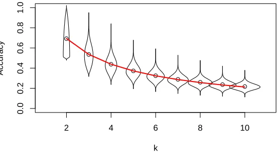
numerically computed GAk(h,{Y(1), . . . , Y(k)}) for randomly drawn labelsY(1), . . . , Y(k) iid
∼
N(0,1), and the distributions of GAkfork= 2, . . . ,10 are illustrated in Figure 4. The mean of the distribution of GAk is thek-class average accuracy, AGAk. The theory presented in the next section deals with how to analyze the average accuracy AGAk as a function of k.
3. Extrapolation
The section is organized as follows. We begin by introducing an explicit formula for the average accuracy AGAk. The formula reveals that AGAk is determined by moments of a one-dimensional functionD(u). Using this formula, we can estimateD(u) using subsampled accuracies. These estimates allow us to extrapolate the average generalization accuracy to an arbitrary number of labels.
The result of our analysis is to expose the average accuracy AGAk as the weighted average of a function D(u), where D(u) is independent ofk, and where konly changes the weighting.
One of the assumptions we rely on is the tie-breaking condition, which allows us to neglect specifying the case when margins are tied.
Definition 2 Tie-breaking condition: for allx∈ X,MY(x)6=MY0(x) with probability one
for Y, Y0 independently drawn from π.
In practice, one can simply break ties randomly, which is mathematically equivalent to adding a small amount of random noiseto the function M.
The result is stated as follows.
Theorem 3 Supposeπ,{Fy}y∈Y, and score functionsMy satisfy the tie-breaking condition.
Then, there exists a cumulative distribution functionD(u) defined on the interval[0,1]such
that
AGAk= 1−(k−1)
Z 1
0
D(u)uk−2du. (5)
3.1. Analysis of Average Accuracy
associated score function (MY) and an example vector (X) drawn from labelY. Explicitly, this sampling can be written:
Y ∼π, MY|Y ∼νY, X|Y ∼FY.
Similarly we use (Y0, MY0, X0) and (Y∗, MY∗, X∗) for two more triplets with independent
and identical distributions. Specifically,X∗ will typically note the test example, and there-foreY∗ the true label andMY∗ its score function.
The functionDis related to a favorability function. Favorability measures the probabil-ity that the score for the examplexis going to be maximized by a particular score function
my, compared to a random competitorMY0. Formally, we write
Ux(my) = Pr[my(x)> MY0(x)]. (6)
Note that for fixed example x, favorability is monotonically increasing in my(x). If
my(x)> my†(x), then Ux(y)> Ux(y†), because the event {my(x) > MY0(x)} contains the
event{my†(x)> MY0(x)}.
Therefore, given labels y(1), . . . , y(k) and test instancex, we can think of the classifier as choosing the label with the greatest favorability:
ˆ
y = argmaxy(i)∈Smy(i)(x) = argmaxy(i)∈SUx(my(i)).
Furthermore, via a conditioning argument, we see that this is still the case even when the test instance and labels are random, as long as the random example X∗ is independent of
Y. (Recall that in our notation,X andY are dependent, but X∗⊥Y.)
ˆ
Y = argmaxY(i)∈SMY(i)(X∗) = argmaxY(i)∈SUX∗(M
Y(i)).
The favorability takes values between 0 and 1, and when any of its arguments are random, it becomes a random variable with a distribution supported on [0,1]. In particular, we consider the following two random variables:
a. the incorrect-label favorability Ux∗(MY) between a given fixed test instance x∗, and
the score function of a random incorrect labelMY, and
b. thecorrect-label favorabilityUX∗(MY∗) between a random test instanceX∗, and the
score function of the correct label, MY∗.
3.1.1. Incorrect-Label Favorability
The incorrect-label favorability can be written explicitly as
Ux∗(MY) = Pr[MY(x∗)> MY0(x∗)|MY(x∗)]. (7)
Note that MY and MY0 are identically distributed, and both are unrelated to x∗ that is
fixed. This leads to the following result:
Lemma 4 Under the tie-breaking condition, the incorrect-label favorabilityUx∗(MY)is
uni-formly distributed for any x∗∈ X, meaning
Pr[Ux∗(MY)≤u] =u (8)
Proof Write Ux∗(MY) = Pr[Z > Z0|Z], where Z = MY(x) and Z0 = MY0(x) for
Y, Y0 i.i.d.∼ π. The tie-breaking condition implies that Pr[Z = Z0] = 0. Now observe that
for independent random variables Z, Z0 with Z =D Z0 and Pr[Z =Z0] = 0, the conditional probability Pr[Z > Z0|Z] is uniformly distributed.
3.1.2. Correct-Label Favorability
The correct-label favorability is
U∗ =UX∗(MY∗) = Pr[MY∗(X∗)> MY0(X∗)|Y∗, MY∗(X∗), X∗]. (9)
The distribution of U∗ will depend on π, {Fy}y∈S and {νy}y∈S, and generally cannot be written in a closed form. However, this distribution is central to our analysis–indeed, we will see that the functionDappearing in theorem 3 is defined as the cumulative distribution function of U∗.
The special case of k = 2 shows the relation between the distribution of U∗ and the average generalization accuracy, AGA2. In the two-class case, the average generalization accuracy is the probability that a random correct label score function gives a larger value than a random distractor:
AGA2= Pr[MY∗(X∗)> MY0(X∗)].
where Y∗ is the correct label, and Y0 is a random incorrect label. If we condition onY∗,
MY∗ and X∗, we get
AGA2=E[Pr[MY∗(X∗)> MY0(X∗)|Y∗, MY∗, X∗]].
Here, the conditional probability inside the expectation is the correct-label favorability. Therefore,
AGA2=E[U∗] =
Z
D(u)du,
where D(u) is the cumulative distribution function of U∗, D(u) = Pr[U∗ ≤u]. Theorem 3 extends this to generalk; we now give the proof.
Proof Without loss of generality, suppose that the true label isY∗ and the incorrect labels areY(1), . . . , Y(k−1). We have
AGAk= Pr[MY∗(X∗)> k
−1 max
i=1 MY(i)(X
∗)] = Pr[U∗ >maxk−1 i=1 UX
∗(M
Y(i))],
recalling thatU∗=UX∗(MY∗). Now, if we condition onX∗=x∗,Y∗ =y∗andMY∗ =my∗,
then the random variable U∗ becomes fixed, with value
Therefore,
AGAk=E[Pr[U∗ > k−1 max
i=1 UX
∗(M
Y(i))|X∗ =x∗, Y∗ =y∗, MY∗ =my∗]]
=E[Pr[U∗ >maxk−1 i=1 UX
∗(M
Y(i))|X∗ =x∗, U∗=u∗]].
Now define Umax,k−1 = maxki=1−1UX∗(M
Y(i)). Since by Lemma 4, UX∗(M
Y(i)) are i.i.d.
uniform conditional on X∗=x∗, we know that
Umax,k−1|X∗ =x∗∼Beta(k−1,1). (10)
Furthermore,Umax,k−1 is independent of U∗ conditional onX∗. Therefore, the conditional probability can be computed as
Pr[U∗> Umax,k−1|X∗=x∗, U∗ =u∗] =
Z u∗
0
(k−1)uk−2du.
Consequently,
AGAk=E[Pr[U∗ > k−1 max
i=1 UX
∗(M
Y(i))|X∗ =x∗, U∗=u∗]] (11)
=E[
Z U∗
0
(k−1)uk−2du|U∗ =u∗] (12)
=E[
Z 1
0
I{u≤U∗}(k−1)uk−2du] (13)
= (k−1)
Z 1
0
Pr[u≤U∗]uk−2du (14)
= 1−(k−1)
Z 1
0
Pr[u≥U∗]uk−2du. (15)
By definingD(u) as the cumulative distribution function ofU∗ on [0,1],
D(u) = Pr[UX∗(MY∗)≤u], (16)
and substituting this definition into (15), we obtain the identity (5).
Theorem 3 expresses the average accuracy as a weighted integral of the function D(u). Essentially, this theoretical result allows us to reduce the problem of estimating AGAk to one of estimating D(u). But how shall we estimate D(u) from data? We propose using non-parametric regression for this purpose in Section 3.3.
3.2. Favorability and Average Accuracy for the Toy Example
Recall that for the toy example from Section 2.4, the score functionMy was a non-random function of y that measures the distance between xand ρy
My(x∗) = log(p(x∗|y)) =−
For this model, the favorability functionUx∗(my) compares the distance betweenx∗ and
ρy to the distance betweenx∗ andρY0 for a randomly chosen distractorY0∼N(0,1):
Ux∗(my) = Pr[|ρy−x∗|<|ρY0−x∗|]
= Φ
x∗+|ρy−x∗|
ρ
−Φ
x∗− |ρy−x∗|
ρ
,
where Φ is the standard normal cumulative distribution function. Figure 5(a) illustrates the level sets of the functionUx∗(my). The highest values ofUx∗(my) are near the linex∗ =ρy
corresponding to the conditional mean of X|Y, and as one moves farther from the line,
Ux∗(my) decays. Note, however, that large values of x∗ and y (with the same sign) result
in larger values of Ux∗(my) since it becomes unlikely forY0∼N(0,1) to exceed Y =y.
Using the formula above, we can calculate the correct-label favorabilityU∗ =UX∗(MY∗)
and its cumulative distribution function D(u). The function Dis illustrated in Figure 5(b) for the current example with ρ = 0.7. The red curve in Figure 4 was computed using the formula
AGAk= 1−(k−1)
Z
D(u)uk−2du.
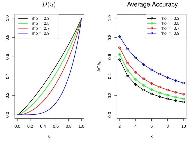
It is illuminating to consider how the average accuracy curves and the D(u) functions vary as we change the parameter ρ. Higher correlations ρ lead to higher accuracy, as seen in Figure 6(a), where the accuracy curves are shifted upward asρ increases from 0.3 to 0.9. The favorabilityUx∗(my) tends to be higher on average as well, which leads to lower values
of the cumulative distribution function–as we see in Figure 6(b), where the function D(u) decreases asρ increases, and therefore accuracy increases.
3.3. Estimation
Next, we discuss how to use data from smaller classification tasks to extrapolate average accuracy. We are seeking an unbiased estimator AGA\k such that
E[AGA\k] = AGAk.
Assume that we have data from a k1-class random classification task, and would like to estimate the average accuracy AGAk2 fork2 > k1 classes. Our estimation method will use
thek-class average test accuracies, ATA2, ...,ATAk1 (see Eq 4), for its inputs.
The key to understanding the behavior of the average accuracy AGAk is the function
D. We adopt a linear model
D(u) = m
X
`=1
β`h`(u), (17)
whereh`(u) are known basis functions, andβ`are the linear coefficients to be estimated. The linearity assumption (17) means that linear regression can be used to estimate the average accuracy curve. This the the idea behind our proposed method ClassExReg, meaning
Ux∗(My)forρ= 0.7 D(u)forρ= 0.7
−2 −1 0 1 2
−3 −2 −1 0 1 2 3
rho = 0.7
x*
y
U > 0.1 U > 0.1
U > 0.2 U > 0.2
U > 0.3 U > 0.3
U > 0.4 U > 0.4 U > 0.5 U > 0.5
U > 0.6
U > 0.6
U > 0.7
U > 0.7
U > 0.8
U > 0.8
U > 0.9
U > 0.9
0.0 0.2 0.4 0.6 0.8 1.0
0.0 0.2 0.4 0.6 0.8 1.0
rho = 0.7
u
K(u)
Figure 5: Favorability for toy example: Left: The level curves of the functionUx∗(My)
in the bivariate normal model withρ= 0.7. Right: The function D(u) gives the cumulative distribution function of the random variableUX∗(MY).
D(u) Average Accuracy
0.0 0.2 0.4 0.6 0.8 1.0
0.0 0.2 0.4 0.6 0.8 1.0 u K(u)
rho = 0.3 rho = 0.5 rho = 0.7 rho = 0.9
2 4 6 8 10
0.0 0.2 0.4 0.6 0.8 1.0 k A G Ak o o o o
rho = 0.3 rho = 0.5 rho = 0.7 rho = 0.9
Figure 6: Average accuracy with different ρ’s: Left: The average accuracy AGAk.
Conveniently, AGAk can also be expressed in terms of the β` coefficients. If we plug in the assumed linear model (17) into the identity (5), then we get
1−AGAk = (k−1)
Z
D(u)uk−2du (18)
= (k−1)
Z 1
0 m
X
`=1
β`h`(u)uk−2du (19)
= m
X
`=1
β`H`,k, (20)
where
H`,k = (k−1)
Z 1
0
h`(u)uk−2du. (21)
The constantsH`,kare moments of the basis functionh`. Note thatH`,kcan be precomputed numerically for anyk≥2.
Now, since the test accuracies ATAk are unbiased estimates of AGAk, this implies that the regression estimate
ˆ
β = argminβ k1
X
k=2
(1−ATAk)− m
X
`=1
β`H`,k
!2
,
is unbiased forβ. The estimate of AGAk2 is similarly obtained from (20), via
\
AGAk2 = 1−
m
X
`=1 ˆ
β`H`,k2. (22)
3.4. Model Selection
Accurate extrapolation using ClassExReg depends on a good fit between the linear model (17) and the true discriminability functionD(u). However, since the functionD(u) depends on the unknown joint distribution of the data, it makes sense to let the data help us choose a good basis {hu}from a set of candidate bases.
Let B1, . . . , Bs be a set of candidate bases, withBi ={h(ui)}mu=1i . Ideally, we would like our model selection procedure to choose the Bi that obtains the best root-mean-squared error (RMSE) on the extrapolation fromk1 tok2 classes. As an approximation, we estimate the RMSE of extrapolation from k1
2 source classes to k1 target classes, by means of the “bootstrap principle.” This amounts to a resampling-based model selection approach, where we perform extrapolations fromk0 =bk21cclasses tok1 classes, and evaluate methods based on how closely the predicted AGA[k1 matches the test accuracy ATAk1. To elaborate, our
model selection procedure is as follows.
1. For`= 1, . . . , L resampling steps:
(a) SubsampleSk(`)
0 from Sk1 uniformly with replacement.
(b) Compute average test accuracies ATA(2`), . . . ,ATA(k`)
0 from the subsampleS
(c) For each candidate basisBi, with i= 1, . . . , s:
i. Compute ˆβ(i,`) by solving the least-squares problem ˆ
β(i,`) = argminβ k0
X
k=2
(1−ATA
(`) k )−
mi X
j=1
βjHj,k(i)
2
.
ii. EstimateAGA[(ki,`1 ) by
[ AGA(ki,`1 )=
mi X
`=1 ˆ
βj(i,`)Hj,k(i) 1.
2. Select the basis Bi∗ by
i∗ = argminsi=1 L
X
`=1
(AGA[(ki,`1 )−ATAk1)
2.
3. Use the basis Bi∗ to extrapolate fromk1 classes (the full data) to k2 classes.
3.5. The Kay KDE-based estimator
In their paper,3 Kay et al. (2008) proposed a method for extrapolating classification ac-curacy to a larger number of classes. The method depends on repeated kernel-density estimation (KDE) steps. Because the method is only briefly motivated in the original text, we present it in our notation.
The idea of the method is to estimate separately for each example x(`i) associated with classy(i) the probability of outscoring a random competitor:
Acc2(x(`i);m) := Pr[m`(i,i)> mY(x(`i))], recalling that we defined m(`i,j) =my(j)(x
(i)
` ). For a given example, accurate classification against k−1 independent (random) distractor classes is equivalent to k−1 independent accurate classifications of a single random competitor. Therefore,
Acck(x(`i);my(i)) := Pr[m
(i,i)
` >maxj6=i m (i,j)
` ] = Acc2(x (i)
` ;my(i))k−1.
Given estimated accuracy valuesa(`i)=Accd2(x
(i)
` ),`= 1, . . . , r,i= 1, ..., k1, we can average thek−1 powers:
[ AGAk=
1 rk1 k1 X i=1 r X `=1
(1−(1−a(`i))k−1) Note that if we have noisy but unbiased estimates of Acc2(x
(i)
` ;my(i)), then the estimates
for Acck(x (i)
` ;my(i)) andAGA[K will be upward biased becauseE[XK]≥E[X]K.
Accuracy for each example Acc2(x(`i)) is estimated in two steps:
1. The density of the wrong-class scores is estimated by smoothing the observed scores with a kernel functionK(·,·) and bandwidthh
ˆ
f`(i)(m) = 1
k1−1
X
j6=i
Kh(m(`i,j), m).
2. The density ˆf`(i)(m) is integrated below the observed true value m(`i,i):
a(`i)=Acc2(d x
(i) ` ) =
Z m(i,i) `
−∞ ˆ
f`(i)(m)dm.
The smoothed density usually over-estimates the size of the right-tail of wrong class distri-bution compared to the observed proportion of errors, biasing downward the accuracy of each individual example.
Briefly, let us point out several key differences between our regression method and Kay’s KDE method:
i. The KDE method balances two biases: an upward bias in exponentiating the estimated accuracy, and a downward bias in smoothing the wrong-class densities. The upward bias occurs because even if Accd2(x
(i)
` ) is unbiased, Accd2(x
(i)
` )k will not be unbiased for Acc2(x(`i))k, and will typically be larger. The bias becomes more prominent for larger k, but decreases as the true accuracy approaches 1. The result of the KDE method therefore depends non-trivially on the choice of smoothing bandwidth used in the density estimation step. (Without smoothing, however, any example that was correctly estimated in the smaller set would have AccdK = 1). The method relies on
smoothing of each class to generate the tail density that exceedsm(`i,i), and therefore it is highly dependent on the choice of kernel bandwidth.
ii. The KDE method estimates the accuracy separately for every class. When the source-set sizekis small, this might lead to less stable estimation for each class and therefore a larger bias after extrapolating. The regression estimator, on the other hand, estimates the average accuracy pooling together information across classes. This might lead to higher variance.
iii. The regression method does not look at the scores directly, only at the rankings. It is therefore blind to monotone transformations on the score functions. The KDE method, on the other hand, is sensitive to the distribution of observed scores.
4. Simulation Study
We ran simulations to check how the proposed extrapolation method, ClassExReg, performs in different settings. The results are displayed in Figure 7. We varied the number of classes k1 in the source data set, the difficulty of classification, and the basis functions. We generated data according to a mixture of isotropic multivariate Gaussian distributions: labelsY were sampled from Y ∼N(0, I10), and the examples for each label sampled from
Similarly to the real-data example, we consider a 1-nearest neighbor classifier, which is given a single training instance per class.
For the estimation, we use the model selection procedure described in Section 3.4 to select the parameterh of the “radial basis”
h`(u) = Φ
Φ−1(u)−t`
h
.
where t` are a set of regularly spaced knots which are determined by h and the problem parameters. Additionally, we add a constant element to the basis, equivalent to adding an intercept to the linear model (17).
The rationale behind the radial basis is to model the density of Φ−1(U∗) as a mixture of Gaussian kernels with varianceh2. To control overfitting, the knots are separated by at least a distance of h/2, and the largest knots have absolute value Φ−1(1− 1
rk2 1
). The size
of the maximum knot is set this way since rk12 is the number of ranks that are calculated and used by our method. Therefore, we do not expect the training data to contain enough information to allow our method to distinguish between more thanrk2
1 possible accuracies, and hence we set the maximum knot to prevent the inclusion of a basis element that has on average a higher mean value than u = 1− 1
rk2 1
. However, in simulations we find that the performance of the basis depends only weakly on the exact positioning and maximum size of the knots, as long as sufficiently large knots are included. As is the case throughout non-parametric statistics, the bandwidthhis the most crucial parameter. In the simulation, we use a grid h={0.1,0.2, . . . ,1}for bandwidth selection.
Meanwhile, for the KDE method, we used a Gaussian kernel, with the bandwidth chosen via pseudolikelihood cross-validation (Cao et al., 1994), as recommended by Kay et al. (2008). Specifically, we used the two methods for cross-validated KDE estimation provided in the stats package in the R statistical computing environment: biased cross-validation and unbiased cross-validation (Scott, 1992).
4.1. Simulation Results
We see in Figure 7 that ClassExReg and the KDE methods with unbiased and biased cross-validation (KDE-UCV, KDE-BCV) perform comparably in the Gaussian simulations. We studied how the difficulty of extrapolation relates to both the absolute size of the number of classes and the extrapolation factor k2
k1. Our simulation has two settings for k1 = {500,5000}, and within each setting we have extrapolations to 2 times, 4 times, 10 times, and 20 times the number of classes.
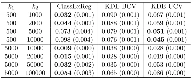
Within each problem setting defined by the number of source and target classes (k1, k2), we use the maximum RMSE across all signal-to-noise settings to quantify the overall per-formance of the method, as displayed in Table 1.
The results also indicate that more accurate extrapolation appears to be possible for smaller extrapolation ratios k2
k1 and larger k1. ClassExReg improves in worst-case RMSE
when moving fromk1= 500 tok1 = 5000 while keeping the extrapolation factor fixed, most dramatically in the case k2
k1 = 2 when it improves from a maximum RMSE of 0.032±0.001
k1 k2 ClassExReg KDE-BCV KDE-UCV 500 1000 0.032(0.001) 0.090 (0.001) 0.067 (0.001) 500 2000 0.044(0.002) 0.088 (0.001) 0.059 (0.001) 500 5000 0.073 (0.004) 0.079 (0.001) 0.051(0.001) 500 10000 0.098 (0.004) 0.076 (0.001) 0.045(0.001) 5000 10000 0.009(0.000) 0.038 (0.000) 0.028 (0.000) 5000 20000 0.015(0.001) 0.028 (0.000) 0.019 (0.000) 5000 50000 0.032(0.002) 0.035 (0.000) 0.053 (0.000) 5000 100000 0.054(0.003) 0.065 (0.000) 0.086 (0.000)
Table 1: Maximum RMSE (se) across all signal-to-noise-levels in predicting TAk2 from k1
classes in multivariate Gaussian simulation. Standard errors were computed by nesting the maximum operation within the bootstrap, to properly account for the variance of a maximum of estimated means.
but also benefiting from at least a 1.8-fold reduction in RMSE when going from the smaller problem to the larger problem in the other three cases.
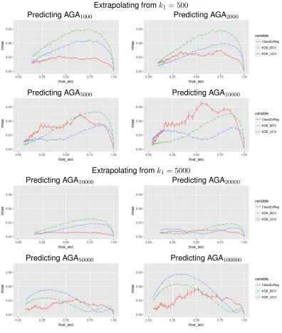
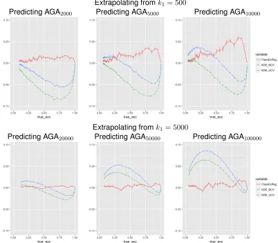
The kernel-density method produces comparable results, but is seen to depend strongly on the choice of bandwidth selection: KDE-UCV and KDE-BCV show very different per-formance profiles, although they differ only in the method used to choose the bandwidth. This matches our analysis in Section 3.5 (item i), where we noted the sensitivity of the tail densities to the bandwidth. Also, the KDE methods show significant estimation bias, as can be seen from Figure 8. As we discussed in 3.5 (item i), this is due to the fact that the KDE method ignores the bias introduced by exponentiation. Meanwhile, ClassExReg avoids this source of bias by estimating the (k−1)st moment ofD(u) directly. As we see in Figure 8, correcting for the bias of exponentiation helps greatly to reduce the overall bias. Indeed, while ClassExReg shows comparable bias for the 500 to 10000 extrapolation, the bias is very well-controlled in all of the k1 = 5000 extrapolations.
5. Experimental Evaluation
We demonstrate the extrapolation of average accuracy in two data examples: (i) predicting the accuracy of a face recognition on a large set of labels from the system’s accuracy on a smaller subset, and (ii) extrapolating the performance of various classifiers on an optical character recognition (OCR) problem in the Telugu script, which has over 400 glyphs.
The face-recognition example takes data from the “Labeled Faces in the Wild” data set (Huang et al. (2007)), where we selected the 1672 individuals with at least 2 face photos. We form a data set consisting of photo-label pairs (x(ji), y(i)) fori= 1, . . . ,1672 andj= 1,2 by randomly selecting 2 face photos for each individual. We used the OpenFace (Amos et al. (2016)) embedding for feature extraction.4 In order to identify a new photo x∗, we obtain the feature vectorg(x∗) from the OpenFace network, and guess the label ˆywith the
Extrapolating fromk1 = 500
Predicting AGA1000 Predicting AGA2000
Predicting AGA5000 Predicting AGA10000
Extrapolating fromk1 = 5000
Predicting AGA10000 Predicting AGA20000
Predicting AGA50000 Predicting AGA100000
Extrapolating fromk1 = 500
Predicting AGA2000 Predicting AGA5000 Predicting AGA10000
Extrapolating fromk1 = 5000
Predicting AGA20000 Predicting AGA50000 Predicting AGA100000
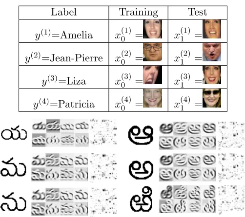
Label Training Test
y(1)=Amelia x(1)0 = x(1)1 =
y(2)=Jean-Pierre x(2)0 = x(2)1 =
y(3)=Liza x(3)0 = x(3)1 =
y(4)=Patricia x(4)0 = x(4)1 =
Figure 9: Face recognition setup (top): Examples of labels and features from the
La-beled Faces in the Wild data set. Telugu OCR (bottom): exemplars from six
of the glyph classes, along with intermediate features and final transformations from the deep convolutional network.
minimal Euclidean distance betweeng(y(i)) andg(x∗), which implies a score function
My(i)(x∗) =−||g(x
(i)
1 )−g(x ∗
)||2.
In this way, we can compute the test accuracy on all 1672 classes, TA1672, but we also subsamplek1={100,200,400} classes in order to extrapolate fromk1 to 1672 classes.
In the Telugu optical character recognition example (Achanta and Hastie (2015)), we consider the use of three different classifiers: logistic regression, linear support-vector ma-chine (SVM), and a deep convolutional neural network.5 The full data consists of 400 classes with 50 training and 50 test observations for each class. We create a nested hierarchy of subsampled data sets consisting of (i) a subset of 100 classes uniformly sampled without replacement from the 400 classes, and (ii) a subset consisting of 20 classes uniformly sam-pled without replacement from the size-100 subsample. We therefore study three different prediction extrapolation problems:
1. Predicting the accuracy on k2 = 100 classes from k1 = 20 classes, comparing the predicted accuracy to the test accuracy of the classifier on the 100-class subsample as ground truth.
is fed into a pre-trained deep convolutional neural network to obtain the 128-dimensional feature vector
g(x). More details are found in Amos et al. (2016).
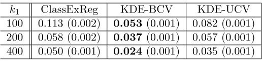
k1 ClassExReg KDE-BCV KDE-UCV 100 0.113 (0.002) 0.053(0.001) 0.082 (0.001) 200 0.058 (0.002) 0.037(0.001) 0.057 (0.001) 400 0.050 (0.001) 0.024(0.001) 0.035 (0.001)
Table 2: Face-recognition extrapolation RMSEs: RMSE (se) on predicting TA1672 from k1 classes
2. Same as (1), but setting k2 = 400 and k1 = 20, and using the full data set for the ground truth.
3. Same as (2), but settingk2= 400 and k1 = 100.
Note that unlike in the case of the face recognition example, here the assumption of marginal classification is satisfied for none of the classifiers. We compare the result of our model to the ground truth obtained by using the full data set.
5.1. Results
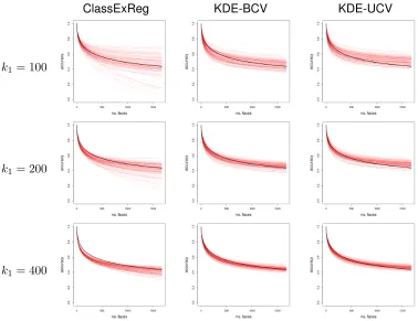
The extrapolation results for the face recognition problem can be seen in Figure 10, which plots the extrapolated accuracy curves for each method for 100 different subsamples of size
k1. As can be seen, for all three methods, the variances decrease rapidly ask1 increases. The root-mean-square errors at k2 = 1672 can be seen in Table 2. KDE-BCV achieves the best extrapolation for all three casesk1 ={100,200,400} with KDE-UCV consistently achieving second place. These results differ from the ranking of the RMSEs for the analagous simulation when predicting k2 = 2000 from k1 = 500 for accuracies around 0.45: in the first row and second column of Figure 7, where the true accuracy is 0.43 (from setting
σ2 = 0.2), the lowest RMSE belongs to KDE-UCV (RMSE=0.0361±0.001), followed closely by ClassExReg (RMSE=0.0372±0.002), and KDE-BCV (RMSE=0.0635±0.001) having the highest RMSE. These discrepancies could be explained by differences between the data distributions between the simulation and the face recognition example, and also by the fact that we only have access to the k2 = 1672-class ground truth for the real data example.
The results for Telugu OCR classification are displayed in Table 3. If we rank the three extrapolation methods in terms of distance to the ground truth accuracy, we see a consistent pattern of rankings between the 20-to-100 extrapolation and the 100-to-400 extrapolation. As we remarked in the simulation, the difficulty of extrapolation appears to be primarily sensitive to the extrapolation ratio k2
k1, which are similar (5 versus 4) in the 20-to-100 and
100-to-400 problems. In both settings, ClassExReg comes closest to the ground truth for the Deep CNN and the SVM, but KDE-BCV comes closest to ground truth for the Logistic regression. However, even for logistic regression, ClassExReg does better or comparably to KDE-UCV.
In the 20-to-400 extrapolation, which has the highest extrapolation ratio (k2
k1 = 20),
ClassExReg KDE-BCV KDE-UCV
k1= 100
k1= 200
k1= 400
Figure 10: Predicted accuracy curves for face-recognition example: The plots show predicted accuracies. Each red curve represents the predicted accuracies using a single subsample of sizek1. The black curve shows the average test accuracy obtained from the full data set.
set, making it difficult to compare extrapolation methods using the 20-to-400 extrapolation task.
Unlike in the face recognition example, we did not resample training classes here, be-cause that would require retraining all of the classifiers–which would be prohibitively time-consuming for the Deep CNN. Thus, we cannot comment on the robustness of the compar-isons from this example, though it is likely that we would obtain different rankings under a new resampling of the training classes.
k1 k2 Classifier True ClassExReg KDE-BCV KDE-UCV 20 100 Deep CNN 0.9908 0.9905 0.7138 0.6507
Logistic 0.8490 0.8980 0.8414 0.8161
SVM 0.7582 0.8192 0.6544 0.5771
20 400 Deep CNN 0.9860 0.9614 0.4903 0.3863 Logistic 0.7107 0.8824 0.7467 0.7015
SVM 0.5452 0.6725 0.5163 0.4070
100 400 Deep CNN 0.9860 0.9837 0.8910 0.8625 Logistic 0.7107 0.7214 0.7089 0.6776
SVM 0.5452 0.5969 0.4369 0.3528
Table 3: Telugu OCR extrapolated accuracies: Extrapolating from k1 to k2 classes in Telugu OCR for three different classifiers: logistic regression, support vector machine, and deep convolutional network
6. Discussion
In this work, we suggest treating the class set in a classification task as random, in order to extrapolate classification performance on a small task to the expected performance on a larger unobserved task. We show that average generalized accuracy decreases with increased label set size like the (k−1)th moment of a distribution function. Furthermore, we introduce an algorithm for estimating this underlying distribution, that allows efficient computation of higher order moments. We additionally implement a kernel-density estimation based extrapolation, and discuss different regimes were the methods are useful. Code for the methods and the simulations can be found inhttps://github.com/snarles/ClassEx.
There are many choices and simplifying assumptions used in the description of the method. Here we discuss these decisions and map some alternative models or strategies for future work.
Two important practical aspects of real-world problems not currently handled by our analysis are (i) non-uniform prior distributions on the labels, and (ii) cost functions other than zero-one loss. In fact, a theory for arbitrary cost functions can double as a theory for non-uniform priors, because the risk incurred under non-uniform priors is equivalent to the risk incurred under a uniform prior but with a weighted cost function. Hence, we address both (i) and (ii) in forthcoming work that shows how performance extrapolation is possible under arbitrary cost functions.
A third direction of exploration is to impose additional modeling assumptions for specific problems. ClassExReg adopts a non-parametric model of the discriminability functionD(u), in the sense thatD(u) was defined via a spline expansion. However, an alternative approach is to assume a parametric family for D(u) defined by a small number of parameters. In forthcoming work, we show that under certain limiting conditions, D(u) is well-described by a two-parameter family. This substantially increases the efficiency of estimation in cases where the limiting conditions are well-approximated.
Acknowledgments
We thank Jonathan Taylor, Trevor Hastie, John Duchi, Steve Mussmann, Qingyun Sun, Robert Tibshirani, Patrick McClure, Francisco Pereira, and Gal Elidan for useful discussion. CZ is supported by an NSF graduate research fellowship, and would also like to thank the European Research Council under the ERC grant agreement n◦[PSARPS-294519] for travel support. We would also like thank the anonymous reviewers for their comments, which improved the readability of the paper.
References
Felix Abramovich and Marianna Pensky. Feature selection and classification of high-dimensional normal vectors with possibly large number of classes. arXiv preprint
arXiv:1506.01567, 2015.
Rakesh Achanta and Trevor Hastie. Telugu OCR framework using deep learning. arXiv
preprint arXiv:1509.05962, 2015.
Brandon Amos, Bartosz Ludwiczuk, and Mahadev Satyanarayanan. Openface: A general-purpose face recognition library with mobile applications. Technical report, CMU-CS-16-118, CMU School of Computer Science, 2016.
Ricardo Cao, Antonio Cuevas, and Wensceslao Gonz´alez Manteiga. A comparative study of several smoothing methods in density estimation. Computational Statistics & Data
Analysis, 17(2):153–176, 1994.
Koby Crammer and Yoram Singer. On the algorithmic implementation of multiclass kernel-based vector machines. Journal of Machine Learning Research, 2(Dec):265–292, 2001.
Justin Davis, Marianna Pensky, and William Crampton. Bayesian feature selection for classification with possibly large number of classes. Journal of Statistical Planning and
Inference, 141(9):3256–3266, 2011.
Jia Deng, Alexander C Berg, Kai Li, and Li Fei-Fei. What does classifying more than 10,000 image categories tell us? In European conference on computer vision, pages 71– 84. Springer, 2010.
Pinar Duygulu, Kobus Barnard, Joao FG de Freitas, and David A Forsyth. Object recogni-tion as machine translarecogni-tion: Learning a lexicon for a fixed image vocabulary. InEuropean
conference on computer vision, pages 97–112. Springer, 2002.
Gregory Griffin, Alex Holub, and Pietro Perona. Caltech-256 object category dataset. 2007.
Maya R Gupta, Samy Bengio, and Jason Weston. Training highly multiclass classifiers.
Journal of Machine Learning Research, 15(1):1461–1492, 2014.
Gary B. Huang, Manu Ramesh, Tamara Berg, and Erik Learned-Miller. Labeled faces in the wild: A database for studying face recognition in unconstrained environments. Technical Report 07-49, University of Massachusetts, Amherst, October 2007.
Kendrick N Kay, Thomas Naselaris, Ryan J Prenger, and Jack L Gallant. Identifying natural images from human brain activity. Nature, 452(March):352–355, 2008.
Yoonkyung Lee, Yi Lin, and Grace Wahba. Multicategory support vector machines: The-ory and application to the classification of microarray data and satellite radiance data.
Journal of the American Statistical Association, 99(465):67–81, 2004.
Maxime Oquab, Leon Bottou, Ivan Laptev, and Josef Sivic. Learning and transferring mid-level image representations using convolutional neural networks. In Proceedings of the
IEEE conference on computer vision and pattern recognition, pages 1717–1724, 2014.
Rui Pan, Hansheng Wang, and Runze Li. Ultrahigh-dimensional multiclass linear discrimi-nant analysis by pairwise sure independence screening.Journal of the American Statistical
Association, 111(513):169–179, 2016.
Sinno Jialin Pan and Qiang Yang. A survey on transfer learning. IEEE Transactions on
knowledge and data engineering, 22(10):1345–1359, 2010.
Francisco Pereira, Bin Lou, Brianna Pritchett, Samuel Ritter, Samuel J Gershman, Nancy Kanwisher, Matthew Botvinick, and Evelina Fedorenko. Toward a universal decoder of linguistic meaning from brain activation. Nature communications, 9(1):963, 2018.
David W. Scott. Multivariate Density Estimation: Theory, Practice, and Visualization. Wiley, 1992.
Claude E. Shannon. A Mathematical Theory of Communication. Bell System Technical
Journal, 27(3):379–423, 1948.
Ali Sharif Razavian, Hossein Azizpour, Josephine Sullivan, and Stefan Carlsson. CNN features off-the-shelf: an astounding baseline for recognition. InProceedings of the IEEE
conference on computer vision and pattern recognition workshops, pages 806–813, 2014.
Efstathios Stamatatos, Walter Daelemans, Ben Verhoeven, Patrick Juola, Aurelio L´ opez-L´opez, Martin Potthast, and Benno Stein. Overview of the author identification task at PAN 2014. In CLEF (Working Notes), pages 877–897, 2014.
Jason Weston and Chris Watkins. Support vector machines for multi-class pattern recog-nition. InESANN, volume 99, pages 219–224, 1999.
Wing H Wong and Li Ma. Optional P´olya tree and Bayesian inference. The Annals of