Maximum Selection and Sorting with Adversarial
Comparators
Jayadev Acharya [email protected]
School of ECE Cornell University Ithaca, NY 14853, USA
Moein Falahatgar [email protected]
ECE Department UC San Diego
La Jolla, CA 92093, USA
Ashkan Jafarpour [email protected]
Sunnyvale, CA 94089, USA
Alon Orlitsky [email protected]
ECE and CSE Departments UC San Diego
La Jolla, CA 92093, USA
Ananda Theertha Suresh [email protected]
Google Research
New York, NY 10011, USA
Editor:Gabor Lugosi
Abstract
We study maximum selection and sorting of nnumbers using imperfect pairwise com-parators. The imperfect comparator returns the larger of the two inputs if the inputs are more than a given threshold apart and an adversarially-chosen input otherwise. We consider two adversarial models: a non-adaptive adversary that decides on the outcomes in advance and an adaptive adversary that decides on the outcome of each comparison depending on the previous comparisons and outcomes.
Against the non-adaptive adversary, we derive a maximum-selection algorithm that uses at most 2n comparisons in expectation and a sorting algorithm that uses at most 2nlnncomparisons in expectation. In the presence of the adaptive adversary, the proposed maximum-selection algorithm uses Θ(nlog(1/)) comparisons to output a correct answer with probability at least 1−, resolving an open problem in Ajtai et al. (2015).
Our study is motivated by a density-estimation problem. Given samples from an un-known distribution, we would like to find a distribution among a un-known class ofncandidate distributions that is close to the underlying distribution in`1distance. Scheffe’s algorithm,
for example, in Devroye and Lugosi (2001) outputs a distribution at an `1 distance at
most 9 times the minimum and runs in time Θ(n2logn). Using our algorithm, the runtime
reduces to Θ(nlogn).
Keywords: noisy sorting, adversarial comparators, density estimation, Scheffe estimator
c
1. Introduction
Maximum selection and sorting are fundamental operations with widespread applications in computing, investment, marketing (Aggarwal et al., 2009), decision making (Thurstone, 1927; David, 1963), and sports. These operations are often accomplished via pairwise comparisons between elements, and the goal is to minimize the number of comparisons.
For example, one may find the largest ofnelements by first comparing two elements and then successively comparing the larger one to a new element. This simple algorithm takes n−1 comparisons, and it is easy to see that n−1 comparisons are necessary. Similarly, merge sort sorts n elements using less than nlogn comparisons, close to the information theoretic lower bound of logn! =nlogn−o(n).
However, in many applications, the pairwise comparisons may be imprecise. For exam-ple, in comparing two random numbers, such as stock performances, or team strengths, the output of the comparison may vary due to chance. Consequently, a number of researchers have considered maximum selection and sorting with imperfect, or noisy, comparators. The comparators in these models mostly function correctly but occasionally may produce an inaccurate comparison result, where the form of inaccuracy is dictated by the application.
Based on the form of inaccuracy, models can be divided into two categories: probabilistic and adversarial. Probabilistic models can be parametric or non-parametric. One of the simplest parametric probabilistic models was considered in Feige et al. (1994), where the output of each comparator could be wrong with some known probability p. Algorithms applying this model for maximum selection were proposed in Adler et al. (1994) and for ranking in Karp and Kleinberg (2007); Ben-Or and Hassidim (2008); Braverman and Mossel (2008); Braverman et al. (2016).
Another parametric family of probabilistic models, the Bradley-Terry-Luce model (Bradley and Terry, 1952) assumes that if two values x and y are compared, then x is selected as the larger with probability x/(x+y). Observe that the comparison is correct with proba-bility max{x, y}/(x+y) ≥ 1/2. Algorithms for ranking and estimating values under this and another related model, the Plackett-Luce (Plackett, 1975; Luce, 2005), are proposed, for example, in Negahban et al. (2012); Sz¨or´enyi et al. (2015). The Mallows model is yet another example of a parametric probabilistic model and is studied in Busa-Fekete et al. (2014).
Non-parametric probabilistic models assume some natural constraints on comparison probabilities, such as Strong Stochastic Transitivity or Stochastic Triangle Inequality. Al-gorithms for maximum selection and sorting under these models are studied in Falahatgar et al. (2017b,a, 2018); Yue and Joachims (2011) and algorithms for comparison-probability matrix estimation are considered in Shah et al. (2016). This model is also considered for the top-k sorting problem in Chen et al. (2017b,a).
We consider a model where, unlike the probabilistic models, the comparison outcome can be adversarial. If the numbers compared are more than a threshold ∆ apart, the comparison is correct, while if they differ by at most ∆, the comparison outcome is arbitrary, and possibly even adversarial.
Weber-Fechner law (Ekman, 1959) stipulates that humans can distinguish between two physical stimuli only when their difference exceeds some threshold (known asjust noticeable difference). Additionally, in sports, a judge or a home-team advantage may, even adversar-ially, sway the outcome of a game between two teams of similar strength but not between teams of significantly different strengths. Our main motivation for the model derives from the important problem of density estimation and distribution learning.
1.1. Density estimation via pairwise comparisons
In a typical PAC-learning setup (Valiant, 1984; Kearns et al., 1994), we are given samples from an unknown distribution p0 in a known distribution class P and would like to find, with high probability, a distribution ˆp∈ P such thatkpˆ−p0k1 < δ.
One standard approach proceeds in two steps (Devroye and Lugosi, 2001):
1. Offline, construct aδ-cover ofP, a finite collectionPδ⊆ P of distributions such that
for any distributionp∈ P, there is a distributionq ∈ Pδ such thatkp−qk1< δ. 2. Using the samples from p0, find a distribution in Pδ whose `1 distance top0 is close
to the`1 distance of the distribution in Pδ that is closest to p0.
These two steps output a distribution whose`1 distance fromp0 isclose toδ. Surprisingly, for several common distribution classes, such as Gaussian mixtures, the number of samples required by this generic approach matches the information theoretically optimal sample complexity, up to logarithmic factors (Daskalakis and Kamath, 2014; Suresh et al., 2014; Diakonikolas et al., 2016).
The Scheffe Algorithm (Scheffe, 1947; Devroye and Lugosi, 2001) is a popular method for implementing the second step, namely to find a distribution inPδ with a small`1 distance from p0. It takes every pair of distributions in Pδ and uses the samples from p0 to decide which of the two distributions is closer to p0. It then declares the distribution that “wins” the most pairwise closeness comparisons to be the nearly-closest top0. As shown in Devroye and Lugosi (2001), the Scheffe algorithm yields, with high probability, a distribution that is at most nine times further fromp0 than the distribution in Pδ with the lowest`1 distance
from p0, plus a diminishing additive term; hence, a distribution that is roughly 9δ away from p0 is found. Since this algorithm compares every pair of distributions in Pδ, it uses
quadratic in|Pδ|comparisons. In Section 6, we use maximum-selection results to derive an
algorithm with the same approximation guarantee but linear in |Pδ|comparisons.
1.2. Organization
2. Notations and preliminaries
Practical applications call for sorting or selecting the maximum of not just numbers, but, rather, of items with associated values—for example, finding the person with the highest salary, the product with the lowest price, or a sports team with the most capability of winning. Associate with each item i a real value xi and let X
def
= {x1, . . . , xn} be the
multiset of values. In maximum selection, we use noisy pairwise comparisons to find an indexisuch that xi is close to the largest element x∗
def
= max{x1, . . . , xn}.
Formally, a faulty comparatorC takes two distinct indices iand j and, if|xi−xj|>∆,
outputs the index associated with the higher value, while if |xi−xj| ≤∆, outputs eitheri
orj, possibly adversarially. Without loss of generality, we assume that ∆ = 1. Then,
C(i, j) =
arg max{xi, xj} if |xi−xj|>1,
iorj (adversarially) if |xi−xj| ≤1.
It is easier to think just of the numbers, rather than the indices. Therefore, informally we will simply view the comparators as taking two real inputsxi and xj, and outputting
C(xi, xj) =
max{xi, xj} if |xi−xj|>1,
xi orxj (adversarially) if |xi−xj| ≤1.
(1)
We consider two types of adversarial comparators: non-adaptive andadaptive.
• A non-adaptive adversarial comparator has complete knowledge of X and the algo-rithm but must fix its outputs for every pair of inputs before the algoalgo-rithm starts
• An adaptive adversarial comparator not only has access to the algorithm and the inputs but is also allowed to adaptively decide the outcomes of the queries taking into account all the previous comparisons made by the algorithm
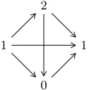
A non-adaptive comparator can be naturally represented by a directed graph with n nodes representing thenindices. There is an edge from nodeito nodej if the comparator declares xi to be larger than xj, namely, C(xi, xj) =xi. Figure 1 is an example of such a
comparator, where, for simplicity, we show only the values 0, 1, 1, 2, and not the indices. Note that, by definition,C(2,0) = 2, but for all the other pairs, the outputs can be decided by the comparator. In this example, the comparator declares the node with value 2 as the “winner” against the right node with value 1 but as the “loser” against the left node, also with value 1. Among the two nodes with value 1, it arbitrarily declares the left one as the winner. An adaptive adversary reveals the edges one-by-one as the algorithm proceeds.
We refer to each comparison as aquery. The number of queries an algorithmAmakes for
X ={x1, . . . , xn}is itsquery complexity, denoted byQAn.1 Our algorithms are randomized,
and QAn is a random variable. The expected query complexity ofA for the input X is
qnAdef= E[QAn],
where the expectation is over the randomness of the algorithm. Note that the expected query complexity is defined for all runs of an algorithm, and it is independent of the success probability.
2
1
0 1
Figure 1: Comparator for four inputs with values {0,1,1,2}
LetCnon(X), or simplyCnon, be the set of all non-adaptive adversarial comparators, and let Cadpt be the set of all adaptive adversarial comparators. The maximum expected query
complexity of A against non-adaptive adversarial comparators is
qAn,non def= max
C∈Cnon max
X q A
n. (2)
Similarly, the maximum expected query complexity of Aagainst adaptive adversarial com-parators is
qAn,adpt def= max
C∈Cadpt max
X q A
n.
We evaluate an algorithm by how close its output is to x∗ (the maximum ofX). Definition 1 A number x is a t-approximation of x∗ ifx≥x∗−t.
The t-approximation error of an algorithm A overninputs is
EnA(t)def= Pr (YA(X)< x∗−t),
the probability thatA’s outputYA(X) isnot at-approximation ofx∗. For an algorithmA,
the maximum t-approximation error for the worst non-adaptive adversary is
EnA,non(t)def= max
C∈Cnon max
X E A
n(t),
and, similarly, for the adaptive adversary,
EnA,adpt(t)def= max
C∈Cadpt max
X E A
n(t).
For the non-adaptive adversary, the minimum t-approximation error of any algorithm is
Ennon(t)def= min
A E A,non
n (t),
and, similarly, for the adaptive adversary,
Enadpt(t)def= min
A E A,adpt
n (t).
Since adaptive adversarial comparators are stronger than non-adaptive, for all t,
Enadpt(t)≥ Ennon(t). Example 1 shows thatEnon
Example 1 Enon
3 (t)≥ 13 for all t <2. Consider X ={0,1,2} and the following
compara-tors. .
0
1 2
By symmetry, no algorithm can differentiate between the three inputs. Hence, any algorithm will output 0 with probability 1/3.
3. Previous and new results In Section 4.1 we lower bound Enon
n (t) as a function of t. In Lemma 2, we show that for all
t < 1 and odd n,Enon
n (t) = 1−1/n, namely for some X, approximating the maximum to
within less than one is equivalent to guessing a randomxias the maximum. In Lemma 3, we
modify Example 1 and show that for allt <2 and oddn, any algorithm hast-approximation error close to 1/2 for some input.
We propose a number of algorithms to approximate the maximum. These algorithms have different guarantees in terms of the probability of error, approximation factor, and query complexity.
We first consider two simple algorithms: the complete tournament, denotedcompl, and the sequential selection, denoted seq. Algorithm compl compares all the possible input pairs and declares the input with the most wins as the maximum. We show the simple result that compl outputs a 2-approximation of x∗. We then consider the algorithm seq that compares a pair of inputs, discards the loser, and compares the winner with a new input. We show that even under random selection of the inputs, there exist inputs such that, with high probability, seqcannot provide a constant approximation to x∗.
We then consider more advanced algorithms. The knock-out algorithm, at each stage, pairs the inputs at random and keeps the winners of the comparisons for the next stage. We design a slight modification of this algorithm, denoted ko-mod that achieves a 3-approximation with error probability at most , even against adaptive adversarial com-parators. We note that Ajtai et al. (2015) proposed a different algorithm with similar performance guarantees.
Motivated by quick-sort, we propose a quick-select algorithm q-select that outputs a 2-approximation with zero error probability. It has an expected query complexity of at most 2nagainst the non-adaptive adversary. However, in Example 2, we see that this algorithm requires n2
queries against the adaptive adversary.
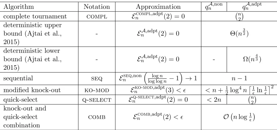
This leaves the question of whether there is a randomized algorithm for 2-approximation of x∗ with O(n) queries against the adaptive adversary. In fact, Ajtai et al. (2015) pose this as an open question. We resolve this problem by designing an algorithm comb that combines quick-select and knock-out. We prove thatcomboutputs a 2-approximation with probability of error, at most, , using O(nlog1) queries. We summarize the results in Table 1.
Algorithm Notation Approximation qAn,non qAn,adpt
complete tournament compl Encompl,adpt(2) = 0 n2
deterministic upper bound (Ajtai et al., 2015)
- EnA,adpt(2) = 0 Θ(n
3 2)
deterministic lower bound (Ajtai et al., 2015)
- EnA,adpt(2) = 0 - Ω(n
4 3)
sequential seq Enseq,non
logn
log logn−1
→1 n−1
modified knock-out ko-mod Enko-mod,adpt(3)< < n+12log4n
1
ln
1
2
quick-select q-select Enq-select,adpt(2) = 0 <2n n2
knock-out and quick-select combination
comb Encomb,adpt(2)< O nlog1
Table 1: Maximum selection algorithms
algorithm for 2-approximation of the maximum using only O(n3/2) queries. Moreover, they prove that no deterministic algorithm with fewer than Ω(n4/3) queries can output a 2-approximation ofx∗ for the adaptive adversarial model.
4. Simple results
In Lemmas 2 and 3, we prove lower bounds on the error probability of any algorithm that provides a t-approximation of x∗ for t < 1 and t < 2, respectively. We then consider two straightforward algorithms for finding the maximum. One is the complete tournament, where all pairs of inputs are compared, and the other is sequential, where inputs are com-pared sequentially, and the loser is discarded at each comparison.
4.1. Lower bounds
We show the following two results:
• Enon
n (t) = 1− 1n for all 0≤t <1 and odd n
• Enon
n (t)≥ 12 − 1
2n for all 1≤t <2 and odd n
These lower bounds can be applied to n, which is even, by adding an extra input that is smaller than all the other inputs and loses to them.
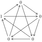
Lemma 2 For all 0≤t <1 and odd n,
Ennon(t) = 1− 1
1
0
0
0 0
Figure 2: Tournament for Lemma 2 whenn= 5
2
0
0
1 1
Figure 3: Tournament for Lemma 3 whenn= 5
Proof Let (x1, x2, . . . , xn) be an unknown permutation of (1,0, . . . ,0
| {z }
n−1
). Suppose we consider
an adversary that ensures each input wins exactly (n−1)/2 times. An example is shown in Figure 2 forn= 5.
To get a lower bound on the performance of any randomized algorithm, we use Yao’s principle. We consider only deterministic algorithms over a uniformly chosen permutation of the inputs, namely only one of the coordinates is 1, and the remaining are less than 1−t. In this case, if we fix any comparison graph (as in Figure 2), and permute the inputs, the algorithm cannot distinguish between 1 and 0’s, and outputs 0 with probability 1−1/n; therefore, Enon
n (t) ≥ 1 − n1. Also, an algorithm that randomly picks an element as the
maximum achieves the error 1−1/n; hence, the lemma.
Lemma 3 For all 1≤t <2 and odd n,
Ennon(t)≥ 1
2− 1 2n.
Proof Letmbe (n−1)/2. Let (x1, x2, . . . , xn) be an unknown permutation of (2,1, . . . ,1
| {z }
m
,0, . . . ,0
| {z }
m
).
Suppose the adversary ensures that 2 loses against all the 1’s and, indeed, all inputs have exactly (n−1)/2 wins. An example is shown in Figure 3.
Similar to Lemma 2, the inputs are all identical to the algorithm, and, therefore, the algorithm outputs one of the 0’s with probability mn = 12− 1
4.2. Two elementary algorithms
In this section, we analyze two well-known maximum selection algorithms, the complete tournament and the sequential selection. We discuss their strengths and weaknesses and show that there is a trade-off between the query complexity and the approximation guaran-tees of these two algorithms. Another well-known algorithm for maximum selection is the knock-out algorithm, and we discuss a variant of it in Section 5.1.
4.2.1. Complete tournament (round-robin)
As its name evinces, a complete tournament involves a match between every pair of teams. Using this metaphor to competitions, we compare all the n2 input pairs, and the input with maximum wins is declared as the output. If two or more inputs end up with the highest wins, any of them can be declared as the output. This algorithm is formally stated incompl.
input: X
compare all input pairs inX, count the number of times each input wins output: an input with the maximum number of wins
Algorithm compl- Complete tournament
Lemma 4 shows that compl gives a 2-approximation against both adversaries. The result, although weaker than the deterministic guarantees of Ajtai et al. (2015), is illustrative and useful in the algorithms proposed later.
Lemma 4 qcompl,adpt
n = n2
andEcompl,adpt
n (2) = 0.
Proof The number of queries is clearly n2. To show Ecompl,adpt
n (2) = 0, note that if
y < x∗−2, then for allz that y wins over,z≤y+ 1< x∗−1, and thereforex∗ also beats them. Since x∗ wins over y, it wins over more inputs than y, and y cannot be the output of the algorithm. It follows that the input with maximum wins is a 2-approximation ofx∗.
compl is deterministic, and, after n2 queries, it outputs a 2-approximation of x∗. If the comparators are noiseless, we can simply compare the inputs sequentially, discarding the loser at each step, and, thus, requiring onlyn−1 comparisons. This evokes the hope of finding a deterministic algorithm that requires a linear number of comparisons and outputs a 2-approximation of x∗. As mentioned earlier, however, Ajtai et al. (2015) showed it is not achievable, as they proved that any deterministic 2-approximation algorithm requires Ω(n4/3) queries. They also showed a strictly superlinear lower bound on any determin-istic constant-approximation algorithm. They designed a determindetermin-istic 2-approximation algorithm usingO(n3/2) queries.
4.2.2. Sequential selection
input: X
choose a random y∈ X and remove it from X
while X is not empty
choose a randomx∈ X and remove it from X
y← C(x, y) end while output: y
Algorithmseq - Sequential selection
Lemma 5 shows that even against the non-adaptive adversary, the algorithm cannot output a constant-approximation ofx∗.
Lemma 5 Let s= log loglognn. For all t < s,
Eseq,non
n (t)≥1−
1 log logn.
Proof Assume that s, logn, and log logn are integers and
xi=
s fori= 1, s−1 fori= 2, . . . , r, s−2 fori=r+ 1, . . . , r2, ..
.
m fori=rs−m−1+ 1, . . . , rs−m, ..
.
0 fori=rs−1+ 1, . . . , rs,
wherer = logn. Consider the following non-adaptive adversarial comparator:
C(xi, xj) =
max{xi, xj} if|xi−xj|>1,
min{xi, xj} if|xi−xj| ≤1. (3)
The sequential algorithm takes a random permutation of the inputs. It then starts by comparing the first two elements and then sequentially compares the winner with the next element, and so on. Let Lj be the location in the permutation where input j appears
for the last time. The next two observations follow from the construction of inputs and comparators respectively.
Observation 1 Input j appears at least (logn−1)times that of input j+ 1.
Observation 2 For the adversarial comparator defined in (3), ifL0> L1> . . . > Ls, then
As a consequence of Observation 1, in the random permutation of inputs, Lj > Lj+1 with probability at least 1−log1n. By the union bound,L0> L1> . . . > Lswith probability
at least,
1− s
logn = 1− 1 log logn.
By applying Observation 2,seq outputs 0 with probability at least 1− log log1 n.
5. Algorithms
In the previous section, we saw that the complete tournament, compl, always outputs a 2-approximation but has quadratic query complexity, while the sequential selection, seq, has linear query complexity but a poor approximation guarantee. A natural question to ask is whether there exist algorithms with bounded error and linear query complexity. In this section, we propose algorithms with linear query complexity and approximation guarantees that compete with the best possible, namely, 2-approximation of x∗.
We propose three algorithms with different performance guarantees:
• Modified knock-out, described in Section 5.1, has linear query complexity, and, with high probability, outputs a 3-approximation of x∗ against both adaptive and non-adaptive adversaries
• Quick-select, described in Section 5.2, outputs a 2-approximation to x∗ (against both adversaries). It also has a linear expected query complexity against non-adaptive adversarial comparators
• Knock-out and quick-select combination, described in Section 5.3, has linear query complexity, and, with high probability, outputs a 2-approximation of x∗ even against adaptive adversarial comparators
We now go over these algorithms in detail.
5.1. Modified knock-out
For simplification, in this section, we assume that lognis an integer. The knock-out algo-rithm derives its name from knock-out competitions where the tournament is divided into logn successive rounds. In each round, the inputs are paired at random, and the winners advance to the next round. Therefore, in roundi, there are 2in−1 inputs. The winner at the end of logn rounds is declared as the maximum.
input at that round, there is a fair chance that the largest input will be eliminated. If this elimination happens in several rounds, we will end up with a number significantly smaller thanx∗.
To circumvent the problem of discarding large inputs, we select a specified number of inputs at each round and save them for the very end, thereby ensuring that at every round, if the largest input is eliminated, then an input within 1 from it has been saved. We then perform a complete tournament on these saved inputs. The algorithm is explained in ko-mod.
input: X
pair the inputs of X randomly, letX0 be the winners output: X0
Algorithmko-sub- Subroutine for ko-mod and comb
input: X,
Y =∅,n1 =1 ln1 ·logn while |X |> n1
randomly choosen1 inputs from X andcopy them to Y
X ←ko-sub(X) end while
output: compl(X ∪ Y)
Algorithmko-mod - Modified knock-out algorithm
In Theorem 6, we show that ko-mod has a 3-approximation error less than.
We first explain the algorithm and then state the result. Let n1 def= 1ln1 ·logn. At each round, we add n1 of the remaining inputs at random to the multiset Y and run the knock-out subroutine ko-sub on the multiset X. When|X | ≤ n1, we perform a complete tournament onX ∪ Yand declare the output as the winner. We show that, with probability at least 1−, the final set Y contains at least one input which is a 1-approximation ofx∗. Since the complete tournament outputs a 2-approximation of its maximum input, ko-mod outputs a 3-approximation ofx∗ with probability greater than 1−.
Theorem 6 Forn1 ≥2, we haveqnko-mod,adpt < n+12(log4n)·
1
ln
1
2
andEko-mod,adpt
n (3)<
.
Proof The number of comparisons made by ko-sub is at most n2 + n4 + n8 +. . . < n. Observe thatko-subis calledmdef=
l
lognn 1
m
times. LetXi be the multisetX at the start of
compl. Then,
|Xm+1∪ Ym+1| ≤ |Xm+1|+|Ym+1|
≤n1+
m
X
i=1
(|Yi+1| − |Yi|)
≤n1+mn1
= log n n1 + 1 · 1 ln 1 ·logn
≤ log n n1 + 1 · 1 ln 1
dlogne
≤log2n·
1 ln 1 ,
where the last inequality follows as n1 ≥ 2 and logn is an integer. Since the complete tournament is quadratic in the input size, the total number of queries is at most n+
1 2log
4n1
ln
1
2
.
Next, we bound the error ofko-mod. Let
X∗def= {x∈ X :x≥x∗−1}
be the multiset of all inputs that are at least x∗−1. For i≤m+ 1, let Xi∗ =Xi∩ X∗ and
Ym∗+1 = Ym+1∩ X∗. Let αi
def = |X
∗
i|
|Xi| and α = max{α1, α2, . . . , αm}. We show that, with high probability, |Xm∗+1∪ Ym∗+1| ≥1, namely, some input inXm+1∪ Ym+1 belongs toX∗. In particular, we show that, with probability 1−, for largeα, |Ym∗+1|>0, and for small α,x∗ ∈ Xm+1. Observe that
Pr(x∗∈ X/ m∗+1) =
m
X
i=1
Pr(x∗ ∈ X/ i∗+1|x∗ ∈ Xi)·Pr(x∗∈ Xi)
≤
m
X
i=1
Pr(x∗ ∈ X/ i∗+1|x∗ ∈ Xi) (a)
≤
m
X
i=1
|Xi∗| −1
|Xi| −1
≤ m X i=1 αi ≤αm,
where (a) follows since at round i, ko-sub randomly pairs the inputs and only inputs in Xi∗\{x∗} are able to eliminate x∗. Next we discuss Pr(|Ym∗+1| = 0). At round i, the probability that an input in X∗ is not picked up in Y is
|Xi|−|Xi∗|
n1
|Xi|
n1
≤
1−|X
∗
i |
|Xi|
n1
Therefore,
Pr(|Ym∗+1|= 0)≤
m
Y
i=1
(1−αi)n1
≤min
i (1−αi) n1
= (1−α)n1.
As a result,
Pr(|Xm∗+1∪ Ym∗+1|= 0) = Pr(|Xm∗+1|= 0 ∧ |Ym∗+1|= 0)
≤Pr(x∗∈ X/ m∗+1 ∧ |Ym∗+1|= 0)
≤max
α min{Pr(x
∗ /
∈ Xm∗+1),Pr(|Ym∗+1|= 0)} ≤max
α min{αm,(1−α) n1}
(a)
≤ max{αm,(1−α)n1}|
α=logn = max
m logn,
1−
logn
n1
(b) < ,
where (a) follows since the first argument of the min increases and the second argument decreases withα. Also, (b) follows sincem≤logn andn1 =1 ln1 logn.
So far, we have shown that with probability 1−, there exists a 1-approximation of x∗ inXm+1∪ Ym+1. From Lemma 4,compl gives a 2-approximation of the maximum input. Consequently, with probability 1−,ko-mod outputs a 3-approximation ofx∗.
In Appendix A, we show that ko-mod cannot output better than 3-approximation of x∗ with constant probability.
5.2. Quick-select
Motivated by quick-sort, we propose a quick-select algorithmq-selectthat at each round compares all the inputs with a random pivot to provide stronger performance guarantees against the non-adaptive adversary.
input: X
pick a pivotxp ∈ X at random
compare xp with all other inputs inX
let Y ⊂ X \{xp}be the multiset of inputs that beat xp
output: ifY 6=∅ output Y otherwise output {xp}
Algorithmqs-sub - Subroutine for q-selectand comb
input: X
while |X |>1
X ←qs-sub(X) end while
output: the unique input inX
Algorithm q-select- Quick-select
eliminated if a 1-approximation of x∗ is chosen as pivot, and, therefore, only inputs that are 2-approximation of x∗ will survive.
Lemma 7 Eq-select,adpt
n (2) = 0.
Proof If the output is x∗, the lemma holds. Otherwise, x∗ is discarded when it was chosen as a pivot or compared with a pivot. Let xp be the pivot when x∗ is discarded;
hence, xp ≥ x∗ −1. By the algorithm’s definition, all the surviving inputs are at least
xp−1≥x∗−2.
We now show that the expected query complexity of q-select against a non-adaptive adversary is at most 2n. This result follows from the observation that the non-adaptive adversary fixes the comparison graph at the beginning, and hence a random pivot wins against half of the inputs in expectation. This idea is made rigorous in the proof of Lemma 8. In Example 2 we show an instance for which q-select requires n2 queries against the adaptive adversary.
Lemma 8 qq-selectn ,non <2n.
Proof Recall that the non-adaptive adversary can be modeled as a complete directed graph where each node is an input and there is an edge from x toy ifC(x, y) =x. Let in(x) be the in-degree of x in such a graph.
At round i, the algorithm chooses a pivot xp at random and compares it to all the
remaining inputs. By keeping the winners, max{in(xp),1} inputs will remain for the next
round. As a result, we have the following recursion for non-adaptive adversaries:
qq-select
n =E[Qq-selectn ]
=n−1 + 1 n
n
X
i=1
E
h
Qq-select in(xi)
i
=n−1 + 1 n
n
X
i=1
By (2),
qq-select,non
n = maxC∈C
non max X q q-select n (4) = max C∈Cnon max X "
n−1 + 1 n
n
X
i=1
qq-selectin(xi)
#
≤n−1 +1 n n X i=1 max C∈Cnon max X q q-select in(xi) =n−1 +1
n
n
X
i=1
qq-selectin(xi) ,non,
where the inequality follows as the maximum of sums is at most the sum of maxima. We prove by strong induction that qq-select,non
n ≤2(n−1), which holds for n= 1. Suppose it
holds for all n0 < n, then,
qq-select,non
n ≤n−1 +
1 n
n
X
i=1
qin(q-selectxi) ,non
≤n−1 + 1 n
n
X
i=1
2·in(xi)
=n−1 +n(n−1) n
≤2(n−1),
where the equality follows since the in-degrees sum to n(n2−1).
Lemma 8 shows thatqq-select,non
n <2n. Next, we show a naive concentration bound for
the query complexity of q-select. By Markov’s inequality, for a non-adaptive adversary,
Pr(Qq-select
n >4n)≤
1 2.
Letk be an integer multiple of 4. Now suppose we runq-select, allowingknqueries. At each 4nqueries, the q-select ends with probability≥ 12. Therefore,
Pr(Qq-select
n > kn)≤2−
k 4.
This naive bound is exponential in k. The next lemma shows a tighter super-exponential concentration bound on the query complexity of the algorithm beyond its expectation. We defer the proof to appendix B.
Lemma 9 Let k0 = max{e, k/2}. For a non-adaptive adversary, Pr(Qq-select
n > kn) ≤
e−(k−k0) lnk0.
Example 2 Let X = {0,0, . . . ,0}. At each round, the adversary declares the pivot to be smaller than all the other inputs. Consequently, only the pivot is eliminated, and the query complexity is n2.
5.3. Knock-out and quick-select combination
ko-mod has the benefit of reducing the number of inputs exponentially at each round and therefore maintaining a linear query-complexity while having only a 3-approximation guarantee. On the other side, q-select has a 2-approximation guarantee while it may require O(n2) queries for some instances of inputs. In comb we combine the benefits of these algorithms and avoid their shortcomings. By carefully repeating qs-sub, we try to reduce the number of inputs by a fraction at each round and keep the largest element in the remaining set. If the number of inputs is not reduced by a fraction, most of them must be close to each other. Therefore, repeating the ko-sub for a sufficient number of times and keeping the inputs with the higher number of wins will guarantee the reduction of the input size without making the approximation error worse. Our final algorithm comb provides a 2-approximation of x∗, even against the adaptive-adversarial comparator and has linear query complexity. Therefore, an open question of Ajtai et al. (2015) is resolved.
input: X,
β1 = 9,β2= 25, i= 0 while |X |>1
i=i+ 1 (iis the round) ni=|X |
runX ←qs-sub(X) for β1log1
times
Xi=X
if |Xi|> 23ni
runko-subonfixed X for
j
β2 43
i
log1ktimes if there exists an input with> 34jβ2 43ilog1kwins
let X be a multiset of inputs with > 34
j
β2 43ilog1
k
wins else
let X be an input with highest number of wins end while
output: X
Algorithmcomb- Knock-out and quick-select combination
We begin the algorithm’s analysis with a few lemmas.
Lemma 10 At each round|X | reduces by at least a third, namely, ni+1 ≤ 23ni.
Proof If at any round |Xi| ≤ 2
3ni, then the lemma holds, and the algorithm does not callko-sub. On the other hand, ifko-sub is called, then by Markov’s inequality at most two-thirds of the inputs win more than three-fourth of the queries. As a result, at roundi, at least one-third of the inputs inX will be eliminated.
as a pivot guarantees a 2-approximation of x∗. The proof is similar to Lemma 7 and is omitted.
Lemma 11 If x∗ ∈ X, at a call to qs-sub eitherx∗ survives or a pivot from X∗ is chosen where in the latter case, only inputs that are2-approximation ofx∗ will survive.
We showed that at each round, comb reduces |X | by at least a third. As a result, the number of inputs decreases exponentially, and the total number of queries is linear in n. We also show that ifx∗ is eliminated at some round, then, with high probability, the pivot at that round is an input from X∗ . Using Lemma 11, this implies that comb outputs a 2-approximation ofx∗ with high probability.
Theorem 12 qncomb,adpt =O nlog1
and Ecomb,adpt
n (2)< .
Proof We start by analyzing the query complexity of comb. By Lemma 10,
ni ≤n· 23
i−1
.
Therefore, the total number of queries at round iis at most
n 23i−1β1log1 +n2 23i−1β2 43ilog1,
where the first term is for calls to qs-sub, and the second term is for calls to ko-sub. Adding the query complexity of all the rounds,
qcomb,adpt
n ≤nlog1
∞
X
i=1
β1 23
i−1
+ 23β2 89
i−1
≤n(3β1+ 6β2) log1 =O nlog1.
We now analyze the approximation guarantee of comb. We show that at least one of the following events happens with probability greater than 1−.
• comboutputsx∗.
• An input inside X∗ is chosen as a pivot at some round.
Let Xi∗def= Xi∩ X∗ and αi def=
|X∗
i|
|Xi|. We consider the following two cases separately.
• Case 1 There exists anisuch that |Xi|> 32ni and αi> 18.
• Case 2 For alli, either|Xi| ≤ 32ni orαi ≤ 18.
First, we consider Case 1. We show that in this case a pivot from X∗ is chosen with probability > 1 −. Observe that at round i, |X | starts at ni < 32|Xi| and gradually
decreases. On the other hand, in all the
β1log1
calls to qs-sub, |X ∩ X∗| is at least
|Xi∗|=αi|Xi|. Therefore, in all the calls toqs-sub at roundi,
|X ∩ X∗|
|X | ≥
αi|Xi|
3 2|Xi|
LetE be the event of not choosing a pivot fromX∗ at round i. As a result,
Pr(E)≤ 1−2 3αi
j
β1log1
k
≤ 11128 log1
< .
Therefore, in Case 1, with probability at least 1−, a pivot fromX∗ is chosen.
We now consider Case 2. By Lemma 11, during the calls to qs-sub, either x∗ survives or an input fromX∗ is chosen as a pivot. Therefore, we may only lose x∗ without choosing a pivot from X∗, if at some round i, |X
i| > 23ni and x∗ wins less than three-fourth of its
queries during the calls to ko-sub.
Recall that in Case 2, if|Xi|> 23ni thenαi≤ 18. Observe thatx∗ wins against a random
input in Xi with probability greater than > 1−αi, which is at least seven-eighths. Let
Ei0 be the event that x∗ wins fewer than three-quarters of its queries at round i. By the Chernoff bound,
Pr(Ei0)≤exp
−jβ2 43ilog1
k
·D 34||78
≤2
4
3
i
,
where D(p||q) def= plnpq+ (1−p) ln11−−pq is the Kullback-Leibler distance between Bernoulli distributed random variables with parameters p and q, respectively. Assuming < 12, the total probability of missing x∗ without choosing a pivot formX∗ is at most
∞
X
i=1
Pr(E0i)≤
∞
X
i=1 2
4
3
i
< .
This shows that with probability > 1−, either x∗ survives or an input inside X∗ is chosen as a pivot. The theorem follows from Lemma 11.
6. Application to density estimation
Our study of maximum selection with adversarial comparators was motivated by the fol-lowing density estimation problem:
Given aknown setPδ={p1, . . . , pn}ofndistributions andksamples from anunknown
distributionp0, output a distribution ˆp∈ Pδ such that for a small constantC >1 and with high probability,
kpˆ−p0k1≤C·min
p∈Pδ
kp−p0k1+ok(1).
outputs a distribution ˆp∈ Pδ such that
||pˆ−p0||1 ≤3·pmin∈P δ
||p−p0||1+
s
10 log1ε
k . (5)
input: distributionsp1 and p2,k i.i.d. samples of unknown distributionp0 let S={x:p1(x)> p2(x)}
let p1(S) andp2(S) be the probability mass that p1 and p2 assign toS let µS be the frequency of samples in S
output: if|p1(S)−µS| ≤ |p2(S)−µS|outputp1, otherwise output p2 Algorithmscheffe-test- Scheffe test for two distributions
scheffe-testprovides a factor-3 approximation with high probability. The algorithm, as stated in its pseudocode, requires computing pi(S) which can be hard since the
distri-butions are not restricted. However, as noted in Suresh et al. (2014), the algorithm can be made to run in time linear in k. Devroye and Lugosi (2001) also extended scheffe-test forn >2. Their proposed algorithm for n >2 runs scheffe-testfor each pair of distri-butions inPδand outputs the distribution with the maximum wins, where a distribution is
a winner if it is the output of scheffe-test. This algorithm is referred to as the Scheffe tournament. They showed that this algorithm finds a distribution ˆp∈ Pδ such that
||pˆ−p0||1≤9 minp∈P δ
||p−p0||1+ok(1),
and the running time is clearly Θ(n2k)—quadratic in the number of distributions.
Mahalanabis and Stefankovic (2008) showed that the optimal coefficients for the Scheffe algorithms are indeed 3 and 9 forn= 2 andn >2, respectively. They proposed an algorithm with an improved factor-3 approximation for n >2—still running in time Θ(n2), however. They also proposed a linear-time algorithm, but it requires a preprocessing step that runs in time exponential inn.
Scheffe’s method has been used recently to obtain nearly sample optimal algorithms for learning Poisson Binomial distributions (Daskalakis et al., 2012), and Gaussian mix-tures (Daskalakis and Kamath, 2014; Suresh et al., 2014).
We now describe how our noisy comparison model can be applied to this problem to yield a linear-time algorithm with the same estimation guarantee as the Scheffe tournament. Our algorithm uses the Scheffe test as a subroutine. Given a sufficient number of samples, k= Θ(logn), the small term in the RHS of (5) vanishes, andscheffe-test outputs
pi if ||pi−p0||1 < 13||pj−p0||1, pj if ||pj−p0||1< 13||pi−p0||1,
unknown otherwise.
Let xi = −log3||pi−p0||1, then analogously to the maximum selection with adversarial
noise in (1),scheffe-test outputs
max{xi, xj} if|xi−xj|>1,
Given a fixed multiset of samples the tournament results are fixed; hence, this setup is identical to the non-adaptive adversarial comparators. In particular, with probability 1−ε, our quick-select algorithm can find ˆp∈ Pδ such that
||pˆ−p0||1 ≤9·min
p∈Pδ
||p−p0||1,
with running time Θ(nk). Next, we consider the combination ofscheffe-testandq-select in greater detail.
Theorem 13 Combination of scheffe-test and q-select algorithms, with probability 1−ε, results in pˆsuch that
||pˆ−p0||1 ≤9·min
p∈Pδ
||p−p0||1+ 4
s
10 log( n 2)
ε
k .
Proof Let
p∗def= argmin
p∈Pδ
||p−p0||1. Using (5), for each pi and pj in Pδ, with probability 1−ε/ n2
, scheffe-test outputs ˆp such that
||pˆ−p0||1 ≤3· min
p∈{pi,pj}
||p−p0||1+
s
10 log( n 2)
ε
k . (6)
By the union bound (6) holds for all pi and pj with probability at least 1−ε. Similar to
Lemma 7, if p∗ is eliminated, then at some round, q-select has chosen p0 as a pivot such that
p0−p0
1 ≤3· ||p ∗−p
0||1+
s
10 log( n 2)
ε
k . Now after choosingp0 as a pivot, for any distribution p00 that survives,
p00−p0 1≤3·
p0−p0
1+
s
10 log( n 2)
ε
k
≤9· ||p∗−p0||1+ 4
s
10 log( n 2)
ε
k .
7. Noisy sorting
7.1. Problem statement
Consider an Algorithm A for sorting the inputs. The output of A is denoted by YA(X) def= (Y1, Y2, . . . , Yn), a particular ordering of the inputs. Similar to the
maximum-selection problem, at-approximation error is
EnA(t)def= Pr
max
i,j:i>j(Yi−Yj)> t
,
namely, the probability of Yi appearing after Yj in YA while Yi −Yj > t. Note that our
definitions forEnA,non(t), EnA,adpt(t),qAn,adpt, and qnA,non hold the same as before.
In the following, we first revisit the complete tournament with a small modification for the sake of the sorting problem, and we show that, under the adaptive adversarial model, it has zero 2-approximation error and query complexity of n2
. We then discuss the quick-sort algorithmq-sortand show that it has zero 2-approximation error but with improved query complexity for the non-adaptive adversary. We apply the known bounds for the running time of the general quick-sort algorithm withndistinct inputs to find the query complexity of q-sort.
7.2. Complete tournament
The algorithm is similar tocomplin Section 4.2.1, and we refer to it as compl-sort. The only difference is in the output of the algorithm.
input: X
compare all input pairs inX, count the number of times each input wins output: output the inputs in the order of their number of wins, breaking the ties
randomly
Algorithmcompl-sort - Complete tournament
The following lemma—and its proof—is similar to Lemma 4, and, therefore, we skip the proof.
Lemma 14 qncompl-sort,adpt= n2
and Ecompl-sort,adpt
n (2) = 0.
Next, we discuss an algorithm with improved query complexity.
7.3. Quick-sort
Quick-sort is a well-known algorithm and, here, is denoted byq-sort. The expected query complexity of quick-sort with noiseless comparisons and distinct inputs is
f(n)def= 2nlnn−(4−2γ)n+ 2 lnn+O(1), (7) where γ is Euler’s constant (McDiarmid and Hayward, 1996). Note that f(n) is a convex function of n.
the inputs with zero 2-approximation error. Next, in Lemma 16, we show that the expected query complexity of quick-sort with non-adaptive adversarial noise is at most its expected query complexity in the noiseless model.
Lemma 15 Eq-sort,adpt
n (2) = 0.
Proof The proof is by contradiction. Suppose xi > xj + 2, but xj appears before xi
in the output of quick-sort algorithm. Then there must have been a pivot xp such that
C(xi, xp) =xp while C(xj, xp) =xj. Sincexi> xj+ 2 no such a pivot exists.
The quick-sort algorithm chooses a pivot randomly to divide the set of inputs into smaller-size sets. The optimal pivot for noiseless quick-sort is known to be the median of the inputs to balance the size of the remained sets. In fact, it is easy to show that if we choose the median of the inputs as the pivot, the query complexity of quick-sort reduces to less than nlogn. Observe that in a non-adaptive adversarial model, the probability of having balanced sets after choosing pivot increases. As a result, in Lemma 16, we show that the expected query complexity of quick-sort in the presence of noise is upper bounded by f(n).
Lemma 16 qnq-sort,non =f(n)and is achieved when the queries are noiseless and the inputs
are distinct.
Proof Let in(x) and out(x) be the in-degree and out-degree of node x in the complete tournament respectively. For the noiseless comparator with distinct inputs, the in-degrees and out-degrees of inputs are permutation of (0,1, . . . , n−1). We show that
argmax
C∈Cnon max
X q q-sort
n ,
is a comparator whose complete tournament in-degrees and out-degrees are permutations of (0,1, . . . , n−1). For notational simplicity let qn = qnq-sort,non. We have the following
recursion for quick-sort similar to (4):
qn≤n−1 +
1 n
n
X
i=1
qout(xi)+qin(xi). (8)
By induction, we show that the solution to (8) is bounded above byf(n), a convex function of n. The induction holds for n = 0,1, and 2. Now suppose the induction holds for all i < n. Since f(n) is a convex function of n and P
iin(xi) =
P
iout(xi) = n(n−1)
2 , the right hand side of (8) is maximized when the in-degrees and out-degrees take their extreme values, namely, when they are permutation of (0,1, . . . , n−1). Plugging in these values, (8) is equivalent to,
qn≤n−1 +
1 n
n
X
i=1
f(in(xi)) +f(out(xi))
≤n−1 + 1 n
n
X
i=1
where the solution to this recursion is f(n), given in (7). Hence qn is bounded above by
f(n), and the equality happens when the in-degrees and out-degrees are permutations of (0,1, . . . , n−1).
Knuth (1998); Hennequin (1989); McDiarmid and Hayward (1992) show different con-centration bounds for quick-sort. In particular, McDiarmid and Hayward (1992) show that the probability of the quick-sort algorithm requiring more comparisons than (1 +) times its expected query complexity is n−2ln lnn+O(ln ln lnn). Observe that for the non-adaptive adversarial model, the chance of a random pivot cutting the set of inputs into balanced sets increases. As a result, one can show that the analysis in McDiarmid and Hayward (1992) follows automatically. In particular, Lemmas 2.1 and 2.2 in McDiarmid and Hay-ward (1992), which are the basis of their analysis, are valid for our non-adaptive adversarial model. Therefore, their tight concentration bound for quick-sort algorithm can be applied to our non-adaptive adversarial model.
Acknowledgments
The authors would like to thank the editor and anonymous reviewers for their constructive comments, and Jelani Nelson for introducing the authors to the adaptive adversarial model. This work was supported in part by NSF grants CIF-1564355 and CIF-1619448. Part of this work was done while J.Acharya was at MIT, supported by MIT-Shell initiative.
Appendix A. For all t <3, ko-mod cannot output a t-approximation Example 3 shows that the modified knock-out algorithm cannot achieve better than 3-approximation of x∗.
Example 3 Suppose n−2 is multiple of 3 and n is a large number. Let X be a random permutation of
{3,2,2, . . . ,2
| {z }
n−2 3
,1,1, . . . ,1
| {z }
n−2 3
,0,0, . . . ,0
| {z }
n−2 3
,0∗}.
This multiset consists of an input with value zero but specified with 0∗ since this input is going to behave differently from other 0s. Let the adversarial comparator be such that all 0s, except 0∗, and all 2s lose to all 1s, and 3 loses to all 2s. If two inputs of the same value get paired, one of them wins randomly (except in the case of 0∗). By the properties of comparator, it is obvious that any 2 will defeat all zeros, including 0∗. In order to prove our main claim, we make the following arguments and show that each of them happens with high probability:
• Pr(input with value 3 is not present in the final multiset)> 103
• Pr(input 0∗ is present in the final multiset)> 13
Before proving each argument, we show why satisfying all the above statements are sufficient to prove our claim. Consider the final multiset; with high probability, it mainly consists of 1s, and there are a small number of 0s and 2s. Moreover, with probability greater than
1 3 ×
3
10, input with value 3 has been removed before reaching the final multiset, and 0 ∗ has
survived to reach the final multiset. Therefore, if we run algorithm compl on the final multiset, the input 0∗ will have the most wins and be declared as the output. Hence for all
t <3, we haveEko-mod,non
n (t)>constant. Note that we did not try to optimize this constant.
Now we show why each of the arguments above is true. Note that the reasoning made here is in expectation and assuming n is sufficiently large. However, the concentration bounds for all these claims are straightforward and thus omitted.
Lemma 17 With high probability, the fraction of 1s in the final multiset is close to 1, and the fraction of 0s and 2s are very small.
Proof We calculate the expected number of 0s, 1s, and 2s at each step. Let fi(j) be the
fraction of j’s at the end of step i. After each step, we lose an input with value 1 if and only if they are paired with each other. As a result, we have the following recursion:
fi+1(1) = 2·fi(1)
fi(1)
2 + 1−fi(1)
,
where the factor 2on the RHS of the recursion above is due to the fact that at each step we are reducing the number of inputs to half. Starting withf0(1) = 1/3, we get the set of values
{1/3,5/9,65/81,6305/6561∼0.96, ...} for fi(1)s. We can see that the ratio is approaching
1 very fast. More precisely, the fraction of 0s is decreasing quadratically since their only chance of survival is to get paired among themselves. As a result, after a couple of steps, the fraction of zeros is extremely small, and, henceforth, the only chance of survival for 2s becomes getting paired among themselves. Additionally their fraction is going to decrease quadratically afterward. As a result, more samples of 1s will be in the final Y with high probability.
Lemma 18 Pr(input with value 3 is not present in the final multiset)> 103.
Proof The input with value3is going to be removed when it is compared against one of the 2s. There is a slight chance of it surviving if it is chosen randomly for being in the output. Thus, the probability of input 3 being removed from the multiset in the first round is
Pr(input 3 is being removed in the first round)= n−2 3n
1−n1
n
> 3 10, where n1 =
1
ln
1
logn
.
Lemma 19 Pr(input 0∗ is present in the final multiset)> 13.
Proof Similar to the argument made in the proof of Lemma 17, we have the following recursion for fi(2).
fi+1(2) = 2·fi(2)
fi(2)
2 + 1−fi(2)−fi(1)
Thus, we have f0(2) = 1/3, f1(2) = 1/3, f2(2) = 5/27, f3(2) = 85/2187. As we stated in
the proof of Lemma 17, the expected fraction of 2s is decreasing quadratically and
Pr(0∗surviving) = (1−1 3)(1−
1 3)(1−
5 27)(1−
85
2187)· · ·> 1 3, proving the lemma.
Appendix B. Proof of Lemma 9 Abbreviate Qq-select
n by Qn. As in the Chernoff bound proof, for all λ >0,
Pr(Qn> kn)≤ E
[eλQn]
ekλn . (9)
Letλ= n1lnk0and Φ(i)def= E[eλQi]. We prove by induction that Φ(i)≤ek 0λi
. The induction holds for i= 0. Similar to (4), we have the following recursion for Φ(n):
Φ(n)≤ e
λ(n−1) n
n
X
j=1
Φ(in(xj))
≤ e λn n n X j=1
Φ(in(xj)).
Since in(xj)< n, using induction,
eλn n
n
X
j=1
Φ(in(xj))≤
eλn n
n
X
j=1
ek0λin(xj). (10)
Observe thatek0λin(xj)is a convex function of in(xj), and
Pn
j=1in(xj) = n(n
−1)
2 . As a result, the RHS of (10) is maximized when the in-degrees take their extreme values, namely, any permutation of (0,1, . . . , n−1). Therefore,
eλn n
n
X
j=1
ek0λin(xj)≤ e
λn
n
n−1
X
j=0 ek0λj
= e
λn
n
ek0λn−1 ek0λ
−1. Combining the above equations,
Φ(n)≤ e
λn
n
ek0λn−1 ek0λ
−1. Similarly, by induction on 1≤i < n,
Φ(i)≤ e
λi
i
ek0λi−1 ek0λ
In Lemma 20 we show that for 1≤i≤n,
eλi i
ek0λi−1 ek0λ
−1 ≤e
k0λi. (11)
Therefore, Φ(i) ≤ ek0λi for 1 ≤ i ≤ n, and, in particular, Φ(n) ≤ ek0λn. Substituting
E[eλQn] = Φ(n) in (9),
Pr(Qn> kn)≤
ek0λn ekλn
= e
k0lnk0
eklnk0
=e−(k−k0) lnk0. This proves the lemma.
We now prove (11). Let k0= max{e,k2}and λ= n1 lnk0. Lemma 20 For all 1≤i≤n, eλii ek
0
λi−1
ek0λ−1 ≤e
k0λi
.
Proof It suffices to show that for all 0< t≤n,
f(t)def= e
λt
t
1−e−k0λt
ek0λ
−1 <1.
Observe that
lim
t→0f(t) = k0λ ek0λ
−1 ≤1.
On the other hand,
f(n) = e
λn
n
1−e−k0λn ek0λ
−1
≤ k
0
n
1 ek0lnk0/n
−1
≤ k
0
n n k0lnk0
≤1.
Next, we show that f(t) is convex. One can show that,
ln1−e
−u
u , is a convex function ofu. As a result,
ln1−e
−k0λt
is a convex function oft. Observe that lneλt is also convex. Therefore,
ln1−e
−k0λt
t + lne
λt,
is convex. As a result, logarithm of f(t) is convex, and, therefore,f(t) is convex.
We showed thatf(t) is convex,f(t→0)≤1, andf(n)≤1. Therefore, for all 0< t≤n, f(t)≤1.
References
Jayadev Acharya, Ashkan Jafarpour, Alon Orlitksy, and Ananda Theertha Suresh. Sorting with adversarial comparators and application to density estimation. InProceedings of the 2014 IEEE International Symposium on Information Theory (ISIT), 2014.
Micah Adler, Peter Gemmell, Mor Harchol-Balter, Richard M. Karp, and Claire Kenyon. Selection in the presence of noise: The design of playoff systems. In Proceedings of the Fifth Annual ACM-SIAM Symposium on Discrete Algorithms. 23-25 January 1994, Arlington, Virginia, pages 564–572, 1994.
Gagan Aggarwal, S Muthukrishnan, D´avid P´al, and Martin P´al. General auction mechanism for search advertising. InProceedings of the 18th international conference on World wide web, pages 241–250. ACM, 2009.
Mikl´os Ajtai, Vitaly Feldman, Avinatan Hassidim, and Jelani Nelson. Sorting and selection with imprecise comparisons. ACM Trans. Algorithms, 12(2):19:1–19:19, November 2015. ISSN 1549-6325.
Michael Ben-Or and Avinatan Hassidim. The bayesian learner is optimal for noisy binary search (and pretty good for quantum as well). InFoundations of Computer Science, 2008. FOCS’08. IEEE 49th Annual IEEE Symposium on, pages 221–230. IEEE, 2008.
Ralph Allan Bradley and Milton E Terry. Rank analysis of incomplete block designs the method of paired comparisons. Biometrika, 39(3-4):324–345, 1952.
Mark Braverman and Elchanan Mossel. Noisy sorting without resampling. InProceedings of the Nineteenth Annual ACM-SIAM Symposium on Discrete Algorithms. January 20-22, 2008, San Francisco, California, USA, pages 268–276, 2008.
Mark Braverman, Jieming Mao, and S Matthew Weinberg. Parallel algorithms for select and partition with noisy comparisons. In Proceedings of the forty-eighth annual ACM symposium on Theory of Computing, pages 851–862. ACM, 2016.
Xi Chen, Sivakanth Gopi, Jieming Mao, and Jon Schneider. Competitive analysis of the top-k rantop-king problem. In Proceedings of the Twenty-Eighth Annual ACM-SIAM Symposium on Discrete Algorithms, pages 1245–1264. SIAM, 2017a.
Xi Chen, Yuanzhi Li, and Jieming Mao. An instance optimal algorithm for top-k ranking under the multinomial logit model. arXiv preprint arXiv:1707.08238, 2017b.
Constantinos Daskalakis and Gautam Kamath. Faster and sample near-optimal algorithms for proper learning mixtures of gaussians. In Proceedings of the 27th Annual Conference on Learning Theory (COLT), 2014.
Constantinos Daskalakis, Ilias Diakonikolas, and Rocco A Servedio. Learning poisson bi-nomial distributions. In Proceedings of the 44th Symposium on Theory of Computing Conference, STOC 2012, New York, NY, USA, May 19 - 22, 2012, pages 709–728, 2012.
Herbert Aron David. The method of paired comparisons, volume 12. Defence Technical Information Center Document, 1963.
Luc Devroye and Gabor Lugosi. Combinatorial Methods in Density Estimation. Springer -verlag, New York, 2001.
Ilias Diakonikolas, Gautam Kamath, Daniel Kane, Jerry Li, Ankur Moitra, and Alistair Stewart. Robust estimators in high dimensions without the computational intractability. arXiv preprint arXiv:1604.06443, 2016.
G ¨OSta Ekman. Weber’s law and related functions. The Journal of Psychology, 47(2): 343–352, 1959.
Moein Falahatgar, Yi Hao, Alon Orlitsky, Venkatadheeraj Pichapati, and Vaishakh Ravin-drakumar. Maxing and ranking with few assumptions. InAdvances in Neural Information Processing Systems, pages 7060–7070, 2017a.
Moein Falahatgar, Alon Orlitsky, Venkatadheeraj Pichapati, and Ananda Theertha Suresh. Maximum selection and ranking under noisy comparisons. In International Conference on Machine Learning, pages 1088–1096, 2017b.
Moein Falahatgar, Ayush Jain, Alon Orlitsky, Venkatadheeraj Pichapati, and Vaishakh Ravindrakumar. The limits of maxing, ranking, and preference learning. In International Conference on Machine Learning, pages 1426–1435, 2018.
Uriel Feige, Prabhakar Raghavan, David Peleg, and Eli Upfal. Computing with noisy information. SIAM Journal on Computing, 23(5):1001–1018, 1994.
Pascal Hennequin. Combinatorial analysis of quicksort algorithm. Informatique th´eorique et applications, 23(3):317–333, 1989.
Michael Kearns, Yishay Mansour, Dana Ron, Ronitt Rubinfeld, Robert E Schapire, and Linda Sellie. On the learnability of discrete distributions. In Proceedings of the Twenty-Sixth Annual ACM Symposium on Theory of Computing, 23-25 May 1994, Montr´eal, Qu´ebec, Canada, pages 273–282, 1994.
Donald Ervin Knuth. The art of computer programming: sorting and searching, volume 3. Pearson Education, 1998.
R Duncan Luce. Individual choice behavior: A theoretical analysis. Courier Corporation, 2005.
Satyaki Mahalanabis and Daniel Stefankovic. Density estimation in linear time. In Pro-ceedings of the 21st Annual Conference on Learning Theory (COLT), pages 503–512, 2008.
Colin McDiarmid and Ryan Hayward. Strong concentration for quicksort. In Proceedings of the Third Annual ACM/SIGACT-SIAM Symposium on Discrete Algorithms, 27-29 January 1992, Orlando, Florida, pages 414–421, 1992.
Colin McDiarmid and Ryan B Hayward. Large deviations for quicksort. journal of algo-rithms, 21(3):476–507, 1996.
Sahand Negahban, Sewoong Oh, and Devavrat Shah. Iterative ranking from pair-wise comparisons. In Advances in Neural Information Processing Systems 25: 26th Annual Conference on Neural Information Processing Systems 2012. Proceedings of a meeting held December 3-6, 2012, Lake Tahoe, Nevada, United States, pages 2483–2491, 2012.
Jelani Nelson. Personal communication. 2015.
Robin L Plackett. The analysis of permutations. Applied Statistics, pages 193–202, 1975.
Henry Scheffe. A useful convergence theorem for probability distributions. In The Annals of Mathematical Statistics, volume 18, pages 434–438, 1947.
Nihar Shah, Sivaraman Balakrishnan, Aditya Guntuboyina, and Martin Wainwright. Stochastically transitive models for pairwise comparisons: Statistical and computational issues. In International Conference on Machine Learning, pages 11–20, 2016.
Ananda Theertha Suresh, Alon Orlitsky, Jayadev Acharya, and Ashkan Jafarpour. Near-optimal-sample estimators for spherical gaussian mixtures. InAdvances in Neural Infor-mation Processing Systems, pages 1395–1403, 2014.
Bal´azs Sz¨or´enyi, R´obert Busa-Fekete, Adil Paul, and Eyke H¨ullermeier. Online rank elici-tation for plackett-luce: A dueling bandits approach. InAdvances in Neural Information Processing Systems, pages 604–612, 2015.
Louis L Thurstone. A law of comparative judgment. Psychological review, 34(4):273, 1927.