Robust Synthetic Control

Robust Synthetic Control

Muhammad Amjad

Operations Research Center

Massachusetts Institute of Technology Cambridge, MA 02139, USA

Devavrat Shah

Department of Electrical Engineering and Computer Science Massachusetts Institute of Technology

Cambridge, MA 02139, USA

Dennis Shen

Department of Electrical Engineering and Computer Science Massachusetts Institute of Technology

Cambridge, MA 02139, USA

Editor:Peter Spirtes

Abstract

We present a robust generalization of the synthetic control method for comparative case studies. Like the classical method cf. Abadie and Gardeazabal (2003), we present an algorithm to estimate the unobservable counterfactual of a treatment unit. A distinguishing feature of our algorithm is that of de-noising the data matrix via singular value thresholding, which renders our approach robust in multiple facets: it automatically identifies a good subset of donors for the synthetic control, overcomes the challenges of missing data, and continues to work well in settings where covariate information may not be provided. We posit that the setting can be viewed as an instance of the Latent Variable Model and provide the first finite sample analysis (coupled with asymptotic results) for the estimation of the counterfactual. Our algorithm accurately imputes missing entries and filters corrupted observations in producing a consistent estimator of the underlying signal matrix, provided p= Ω(T−1+ζ) for someζ >0; here, pis the fraction of observed data andT is the time interval of interest. Under the same proportion of observations, we demonstrate that the mean-squared error in our counterfactual estimation scales asO(σ2/p+ 1/√T), where σ2 is the variance of the inherent noise. Additionally, we introduce a Bayesian framework to quantify the estimation uncertainty. Our experiments, using both synthetic and real-world datasets, demonstrate that our robust generalization yields an improvement over the classical synthetic control method.

Keywords: Observation Studies, Causal Inference, Matrix Estimation

1. Introduction

On November 8, 2016 in the aftermath of several high profile mass-shootings, voters in California passed Proposition 63 in to law BallotPedia (2016). Prop. 63 “outlaw[ed] the possession of ammunition magazines that [held] more than 10 rounds, requir[ed] background checks for people buying bullets,” and was proclaimed as an initiative for “historic progress to reduce gun violence” McGreevy (2016). Imagine that we wanted to study the impact of Prop. 63 on the rates of violent crime in California.

c

Randomized control trials, such as A/B testings, have been successful in establishing effects of interventions by randomly exposing segments of the population to various types of interventions. Unfortunately, a randomized control trial is not applicable in this scenario since only one California exists. Instead, a statistical comparative study could be conducted where the rates of violent crime in California are compared to a “control” state after November 2016, which we refer to as the post-intervention period. To reach a statistically valid conclusion, however, the control state must be demonstrably similar to California sans the passage of a Prop. 63 style legislation. In general, there may not exist a natural control state for California, and subject-matter experts tend to disagree on the most appropriate state for comparison.

As a suggested remedy to overcome the limitations of a classical comparative study outlined above, Abadie et al. proposed a powerful, data-driven approach to construct a “synthetic” control unit absent of intervention Abadie et al. (2010); Abadie and Gardeazabal (2003); Abadie et al. (2011). In the example above, the synthetic control method would construct a “synthetic” state

of California such that the rates of violent crime of that hypothetical state would best match the rates in California before the passage of Prop. 63. This synthetic California can then serve as a data-driven counterfactual for the period after the passage of Prop. 63. Abadie et al. propose to construct such a synthetic California by choosing a convex combination of other states (donors) in the United States. For instance, synthetic California might be 80% like New York and 20% like Massachusetts. This approach is nearly entirely data-driven and appeals to intuition. For optimal results, however, the method still relies on subjective covariate information, such as employment rates, and the presence of domain “experts” to help identify a useful subset of donors. The approach may also perform poorly in the presence of non-negligible levels of noise and missing data.

1.1 Overview of main contributions.

As the main result, we propose a simple, two-step robust synthetic control algorithm, wherein the first step de-noises the data and the second step learns a linear relationship between the treated unit and the donor pool under the de-noised setting. The algorithm is robust in two senses: first, it is fully data-driven in that it is able to find a good donor subset even in the absence of helpful domain knowledge or supplementary covariate information; and second, it provides the means to overcome the challenges presented by missing and/or noisy observations. As another important contribution, we establish analytic guarantees (finite sample analysis and asymptotic consistency) – that are missing from the literature – for a broader class of models.

Robust algorithm. A distinguishing feature of our work is that of de-noising the observation data via singular value thresholding. Although this spectral procedure is commonplace in the matrix completion arena, it is novel in the realm of synthetic control. Despite its simplicity, however, thresholding brings a myriad of benefits and resolves points of concern that have not been previously addressed. For instance, while classical methods have not even tackled the obstacle of missing data, our approach is well equipped to impute missing values as a consequence of the thresholding procedure. Additionally, thresholding can help prevent the model from overfitting to the idiosyncrasies of the data, providing a knob for practitioners to tune the “bias-variance” trade-off of their model and, thus, reduce their mean-squared error (MSE). From empirical studies, we hypothesize that thresholding may possibly render auxiliary covariate information (vital to several existing methods) a luxury as opposed to a necessity. However, as one would expect, the algorithm can only benefit from useful covariate and/or “expert” information and we do not advocate ignoring such helpful information, if available.

through posterior probabilities.

Theoretical performance. To the best of our knowledge, ours is the first to provide finite sample analysis of the MSE for the synthetic control method, in addition to guarantees in the presence of missing data. Previously, the main theoretical result from the synthetic control literature (cf. Abadie et al. (2010); Abadie and Gardeazabal (2003); Abadie et al. (2011)) pertained to bounding the bias of the synthetic control estimator; however, the proof of the result assumed that the latent parameters, which live in the simplex, have a perfect pre-treatment match in the noisy predictor variables – our analysis, on the other hand, removes this assumption. We begin by demonstrating that our de-noising procedure produces a consistent estimator of the latent signal matrix (Theorems 1, 2), proving that our thresholding method accurately imputes and filters missing and noisy observations, respectively. We then provide finite sample analysis that not only highlights the value of thresholding in balancing the inherent “bias-variance” trade-off of forecasting, but also proves that the prediction efficacy of our algorithm degrades gracefully with an increasing number of randomly missing data (Theorems 3, 7, and Corollary 4). Further, we show that a computationally beneficial pre-processing data aggregation step allows us to establish the asymptotic consistency of our estimator in generality (Theorem 5).

Additionally, we prove a simple linear algebraic fact that justifies the basic premise of synthetic control, which has not been formally established in literature, i.e. the linear relationship between the treatment and donor units that exists in the pre-intervention continues to hold in post-intervention period (Theorem 6). We introduce a latent variable model, which subsumes many of the models previously used in literature (e.g. econometric factor models). Despite this generality, a unifying theme that connects these models is that they all induce (approximately) low rank matrices, which is well suited for our method.

Experimental results. We conduct two sets of experiments: (a) on existing case studies from real world datasets referenced in Abadie et al. (2010, 2011); Abadie and Gardeazabal (2003), and (b) on synthetically generated data. Remarkably, while Abadie et al. (2010, 2011); Abadie and Gardeazabal (2003) use numerous covariates and employ expert knowledge in selecting their donor pool, our algorithm achieves similar results without any such assistance; additionally, our algorithm detects subtle effects of the intervention that were overlooked by the original synthetic control approach. Since it is impossible to simultaneously observe the evolution of a treated unit and its counterfactual, we employ synthetic data to validate the efficacy of our method. Using the MSE as our evaluation metric, we demonstrate that our algorithm is robust to varying levels of noise and missing data, reinforcing the importance of de-noising.

1.2 Related work.

subset of possible controls to units that are within the geographical or economic proximity of the treated unit. Therefore, there is still some degree of subjectivity in the choice of the donor pool. In addition, Hsiao (2014); Hsiao et al. (2011) do not include a “de-noising” step, which is a key feature of our approach. For an empirical comparison between the synthetic control and panel data methods, see Gardeazabal and Vega-Bayo (2016). It should be noted that Gardeazabal and Vega-Bayo (2016) also adapts the panel data method to automate the donor selection process. In this comparison study, the authors conclude that neither the synthetic control method nor the panel data method is vastly superior to the other. They suggest that the synthetic control method may be more useful when there are more time periods and covariates. However, when there is a poor pre-treatment match, the synthetical control method is not feasible while the panel data method can still be used, even though it may suffer from some extrapolation bias. But when a good pre-intervention match is found, the authors conclude that the synthetic control method tends to produce lower MSE, MAPE and mean-error. However, in another comparison study, Wan et al. (2018) compare and contrast the assumptions of both methods and note that the panel data method appears to outperform the synthetic control method in a majority of the simulations they conducted.

Among other notable bodies of work, Doudchenko and Imbens (2016) allows for an additive difference between the treated unit and donor pool, similar to the difference-in-differences (DID) method. Moreover, similar to our exposition, Doudchenko and Imbens (2016) relaxes the convexity aspect of synthetic control and proposes an algorithm that allows for unrestricted linearity as well as regularization. In an effort to infer the causal impact of market interventions, Brodersen et al. (2015) introduce yet another evaluation methodology based on a diffusion-regression state-space

model that is fully Bayesian; similar to Abadie et al. (2010); Abadie and Gardeazabal (2003); Hsiao (2014); Hsiao et al. (2011), their model also generalizes the DID procedure. Due to the subjectivity in the choice of covariates and predictor variables, Ferman et al. (2016) provides recommendations for specification-searching opportunities in synthetic control applications. The recent work of Xu (2017) extends the synthetic control method to allow for multiple treated units and variable treatment periods as well as the treatment being correlated with unobserved units. Similar to our work, Xu (2017) computes uncertainty estimates; however, while Xu (2017) obtains these measurements via a

parametric bootstrap procedure, we obtain uncertainty estimates under a Bayesian framework.

Matrix completion and factorization approaches are well-studied problems with broad applications (e.g. recommendation systems, graphon estimation, etc.). As shown profusely in the literature, spectral methods, such as singular value decomposition and thresholding, provide a procedure to estimate the entries of a matrix from partial and/or noisy observations Cand`es and Recht (2008). With our eyes set on achieving “robustness”, spectral methods become particularly appealing since they de-noise random effects and impute missing information within the data matrix Jha et al. (2010). For a detailed discussion on the topic, see Chatterjee (2015); for algorithmic implementations, see Mazumder et al. (2010) and references there in. We note that our goal differs from traditional matrix completion applications in that we are using spectral methods to estimate a low-rank matrix, allowing us to determine a linear relationship between the rows of the mean matrix. This relationship is then projected into the future to determine the counterfactual evolution of a row in the matrix (treated unit), which is traditionally not the goal in matrix completion applications. Another line of work within this arena is to impute the missing entries via a nearest neighbor based estimation algorithm under a latent variable model framework Lee et al. (2016); Borgs et al. (2017).

Despite its popularity, there has been less theoretical work in establishing the consistency of the synthetic control method or its variants. Abadie et al. (2010) demonstrates that the bias of the synthetic control estimator can be bounded by a function that is close to zero when the pre-intervention period is large in relation to the scale of the transitory shocks, but under the additional condition that a perfect convex match between the pre-treatment noisy outcome and covariate variables for the treated unit and donor pool exists. Ferman and Pinto (2016) relaxes the assumption in Abadie et al. (2010), and derives conditions under which the synthetic control estimator is asymptotically unbiased under non-stationarity conditions. To our knowledge, however, no prior work has provided finite-sample analysis, analyzed the performance of these estimators with respect to the mean-squared error (MSE), established asymptotic consistency, or addressed the possibility of missing data, a common handicap in practice.

2. Background

2.1 Notation.

We will denote _R as the field of real numbers. For any positive integer N, let [N] ={1, . . . , N}. For any vectorv∈Rn, we denote its Euclidean (`2) norm bykvk2, and definekvk

2 2=

Pn i=1v

2 i. We define its infinity norm as kvk_∞ = maxi|vi|. In general, the`p norm for a vector v is defined as

kvk_p=Pn_i=1|vi|p 1/p

. Similarly, for anm×nreal-valued matrixA= [Aij], its spectral/operator norm, denoted bykAk₂, is defined askAk₂= max1≤i≤k|σi|, where k= min{m, n}andσi are the singular values ofA. The Moore-Penrose pseudoinverseA† ofAis defined as

A† = k X

i=1

(1/σi)yixTi, where A= k X

i=1

σixiyTi, (1) with xi and yi being the left and right singular vectors of A, respectively. We will adopt the shorthand notation ofk·k ≡ k·k₂. To avoid any confusions between scalars/vectors and matrices, we will represent all matrices in bold, e.g. A.

Let f andg be two functions defined on the same space. We say that f(x) = O(g(x)) and f(x) = Ω(g(x)) if and only if there exists a positive real numberM and a real numberx0 such that for allx≥x0,

|f(x)| ≤M|g(x)| and |f(x)| ≥M|g(x)|, (2) respectively.

2.2 Model.

The data at hand is a collection of time series with respect to an aggregated metric of interest (e.g. violent crime rates) comprised of both the treated unit and the donor pool outcomes. Suppose we observe N ≥2 units across T ≥2 time periods. We denoteT0 as the number of pre-intervention periods with 1≤T0< T, renderingT−T0as the length of the post-intervention stage. Without loss of generality, let the first unit represent the treatment unit – exposed to the intervention of interest at timet=T0+ 1. The remaining donor units, 2≤i≤N, are unaffected by the intervention for the entire time period [T] ={1, . . . , T}.

LetXitdenote the measured value of metric for unitiat timet. We posit

Xit=Mit+it, (3)

et al. (2016); Aldous (1981); Hoover (1979, 1981), we further posit that for all 2≤i≤N,t∈[T]

Mit=f(θi, ρt), (4)

whereθi ∈Rd1 _andρ

t∈Rd2 _{are latent feature vectors capturing unit and time specific information,}

respectively, for some d1, d2 ≥ 1; the latent function f : Rd1 _×

Rd2 _→

R captures the model

relationship. We note that this formulation subsumes popular econometric factor models, such as the one presented in Abadie et al. (2010), as a special case with (small) constantsd1=d2 andf as a bilinear function.

The treatment unit obeys the same model relationship during the pre-intervention period. That is, fort≤T0

X1t=M1t+1t, (5)

where M1t =f(θ1, ρt) for some latent parameter θ1∈ Rd1_{. If unit one was never exposed to the}

intervention, then the same relationship as (5) would continue to hold during the post-intervention period as well. In essence, we are assuming that the outcome random variables forall unaffected units follow the model relationship defined by (5) and (3). Therefore, the “synthetic control” would ideally help estimate the underlying counterfactual meansM1t=f(θ1, ρt) forT0< t≤T by using an appropriate combination of the post-intervention observations from the donor pool since the donor units are immune to the treatment.

To render this feasible, we make the key operating assumption (as done similarly in literature cf. Abadie et al. (2010, 2011); Abadie and Gardeazabal (2003)) that the mean vector of the treatment unit over the pre-intervention period, i.e. the vectorM₁− = [M1t]t≤T0, lies within the span of the

mean vectors within the donor pool over the pre-intervention period, i.e. the span of the donor mean vectorsM_i−= [Mit]2≤i≤N,t≤T0

1_{. More precisely, we assume there exists a set of weightsβ}∗_∈

RN−1

such that for allt≤T0,

M1t= N X

i=2

βi∗Mit. (6)

This is a reasonable and intuitive assumption, utilized in literature, hypothesizing that the treatment unit can be modeled as some combination of the donor pool. In fact, the set of weightsβ∗ _{are the} very definition of a synthetic control. Note, however, that in contrast to Abadie et al. (2010, 2011); Abadie and Gardeazabal (2003), we do not constrain the weights to be non-negative and sum to 1. This may reduce the interpretability of the synthetic control produced. We discuss ways to increase interpretability using our method in Section 3.4.2.

In order to distinguish the pre- and post-intervention periods, we use the following notation for all (donor) matrices: A = [A−,A+_{], where A}− _{= [A}

ij]2≤i≤N,j∈[T0] andA

+ _{= [A}

ij]2≤i≤N,T0<j≤T

denote the pre- and post-intervention submatrices, respectively; vectors will be defined in the same manner, i.e. Ai = [A−i , A

+

i ], where A −

i = [Ait]t∈[T0] and A

+

i = [Ait]T0<t≤T denote the pre- and

post-intervention subvectors, respectively, for theith donor. Moreover, we will denote all vectors related to the treatment unit with the subscript “1”, e.g. A1= [A−₁, A+₁].

In contrast with the classical synthetic control work, we allow our model to be robust to incomplete observations. To model randomly missing data, the algorithm observes each data pointXitin the donor pool with probabilityp∈(0,1], independently of all other entries. While the assumption that pis constant across all rows and columns of our observation matrix is standard in literature, our results remain valid even in situations where the probability of observation is dependent on the row

1. We note that this is a minor departure from the literature on synthetic control starting in Abadie and Gardeazabal (2003) – in literature, the pre-interventionnoisyobservation (rather than the mean) vector

and column latent parameters, i.e. pij =g(θi, ρj)∈(0,1]. In such situations,pij can be estimated as ˆ

pij using consistent graphon estimation techniques described in a growing body of literature, e.g. see Borgs et al. (2017); Chatterjee (2015); Wolfe and Olhede; Yang et al.. These estimates can then be used in our analysis presented in Section 4.

3. Algorithm

3.1 Intuition.

We begin by exploring the intuition behind our proposed two-step algorithm: (1) de-noising the data: since the singular values of our observation matrix,X= [Xit]2≤i≤N,t∈[T], encode both signal and noise, we aim to discover a low rank approximation of X that only incorporates the singular values associated with useful information; simultaneously, this procedure will naturally impute any missing observations. We note that this procedure is similar to the algorithm proposed in Chatterjee (2015). (2)learningβ∗: using the pre-intervention portion of the de-noised matrix, we learn the linear relationship between the treatment unit and the donor pool prior to estimating the post-intervention counterfactual outcomes. Since our objective is to produce accurate predictions, it is not obvious why the synthetic treatment unit should be a convex combination of its donor pool as assumed in Abadie et al. (2010); Abadie and Gardeazabal (2003); Abadie et al. (2014). In fact, one can reasonably expect that the treatment unit and some of the donor units may exhibit negative correlations with one another. In light of this intuition, we learn the optimal set of weights via linear regression, allowing for both positive and negative elements.

3.2 Robust algorithm (algorithm 1).

We present the details of our robust method in Algorithm 1 below. The algorithm utilizes two hyperparameters: (1) a thresholding hyperparameterµ≥0, which serves as a knob to effectively trade-off between the bias and variance of the estimator, and (2) a regularization hyperameterη≥0 that controls the model complexity. We discuss the procedure for determining the hyperparameters in Section 3.4. To simplify the exposition, we assume the entries ofX are bounded by one in absolute value, i.e. |Xit| ≤1.

3.3 Bayesian algorithm: measuring uncertainty (algorithm 2).

In order to quantitatively assess the uncertainty of our model, we will transition from a frequentist perspective to a Bayesian viewpoint. As commonly assumed in literature, we consider a zero-mean, isotropic Gaussian noise model (i.e. ∼ N(0, σ2I)) and use the square loss for our cost function. We present the Bayesian method as Algorithm 2. Note that we perform step one of our robust algorithm exactly as in Algorithm 1; as a result, we only detail the alterations of step two in the Bayesian version (Algorithm 2).

3.4 Algorithmic features: the fine print.

3.4.1 Bounded entries transformation.

Algorithm 1

Robust synthetic control

Step 1. De-noising the data: singular value thresholding (inspired by

Chatter-jee (2015)).

1. Define

Y

= [

Y

]

with

Y

=

(

X

if

X

is observed

,

0

otherwise.

(7)

2. Compute the singular value decomposition of

Y

:

Y

=

X

i=1

s

u

v

.

(8)

3. Let

S

=

{

i

:

s

≥

µ

}

be the set of singular values above the threshold

µ

.

4. Define the estimator of

M

as

ˆ

M

=

1

ˆ

p

X

i∈S

s

u

v

,

(9)

where ˆ

p

is the maximum of the fraction of observed entries in

X

and

.

Step 2. Learning and projecting

1. For any

η

≥

0, let

ˆ

β

(

η

) = arg min

Y

− 1

−

( ˆ

M

−

₎

_v

+

η

k

v

k

.

(10)

2. Define the counterfactual means for the treatment unit as

ˆ

Algorithm 2

Bayesian robust synthetic control

Step 2. Learning and projecting

1. Estimate the noise variance via (bias-corrected) maximum likelihood, i.e.

ˆ

σ

=

1

T

−

1

T0

X

t=1

(

Y

−

Y

¯

)

,

(12)

where ¯

Y

denotes the pre-intervention sample mean.

2. Compute posterior distribution parameters for an appropriate choice of the prior

α

:

Σ

=

1

ˆ

σ

M

ˆ

−

_{( ˆ}

_M

₎

₊

_α

_I

−

₍₁₃₎

β

=

1

ˆ

σ

Σ

M

ˆ

_Y

1

.

(14)

3. Define the counterfactual means for the treatment unit as

ˆ

M

= ˆ

M

β

.

(15)

4. For each time instance

t

∈

[

T

], compute the model uncertainty (variance) as

range. Specifically, the reverse transformation equates to multiplying the end result by (b−a)/2 and adding by (a+b)/2.

3.4.2 Solution interpretability.

For the practitioner who seeks a more interpretable solution, e.g. a convex combination of donors as per the original synthetic control estimator of Abadie et al. (2010, 2011); Abadie and Gardeazabal (2003), we recommend using an`1-regularization penalty in the learning procedure of step 2. Due to the geometry of LASSO, the resulting estimator will often be a sparse vector; in other words, LASSO effectively performs model selection and selects the most important donors that comprise the synthetic control. LASSO can also be beneficial if the number of donors exceeds the number of pre-treatment time periods. Specifically, for anyη >0, we define the LASSO estimator to be

ˆ

β(η) = arg min v∈RN−1

Y

− 1 −( ˆM

−₎T_v 2

+ηkvk₁.

For the purposes of this paper, we focus our attention on ridge regression and provide theoretical results in Section 4 under the`2-regularization setting. However, a closer examination of the LASSO estimator for synthetic control methods can be found in Li and Bell (2017).

3.4.3 Choosing the hyperparameters.

Here, we discuss several approaches to choosing the hyperparameterµfor the singular values; note that µ defines the set S that includes the singular values we wish to include in the imputation procedure. If it is known a priori that the underlying model is low rank with rank at mostk, then it may make sense to choose µ such that |S| = k. A data driven approach, however, could be implemented based on cross-validation. Precisely, reserve a portion of the pre-intervention period for validation, and use the rest of the pre-intervention data to produce an estimate ˆβ(η) for each of the finitely many choices ofµ(s1, . . . , sN−1). Using each estimate ˆβ(η), produce its corresponding treatment unit mean vector over the validation period. Then, select theµthat achieves the minimum MSE with respect to the observed data. Finally, Chatterjee (2015) provides a universal approach to picking a threshold; similarly, we also propose another such universal threshold, (20), in Section 4.1. We utilize the data driven approach in our experiments in this work.

The regularization parameter,η, also plays a crucial role in learning the synthetic control and influences both the training and generalization errors. As is often the case in model selection, a popular strategy in estimating the idealη is to employ cross-validation as described above. However, since time-series data often have a natural temporal ordering with causal effects, we also recommend employing the forward chaining strategy. Although the forward chaining strategy is similar to leave-one-out (LOO) cross-validation, an important distinction is that forward chaining does not break the temporal ordering in the training data. More specifically, for a particular candidate ofη at every iterationt∈[T0], the learning process uses [Y11, . . . , Y1,t−1] as the training portion while reservingY1t as the validation point. As before, the average error is then computed and used to evaluate the model (characterized by the choice ofη). The forward chaining strategy can also be used to learn the optimalµ.

3.4.4 Scalability.

computational infrastructure, our de-noising procedure, and algorithm in generality, can scale quite well. Also note that for a low rank structure, we typically only need to compute the top few singular values and vectors. Various truncated-SVD algorithms provide resource-efficient implementations to compute the topksingular values and vectors instead of the complete-SVD.

3.4.5 Low rank hypothesis.

The factor models that are commonly used in the Econometrics literature, cf. Abadie et al. (2010, 2011); Abadie and Gardeazabal (2003), often lead to a low rank structure for the underlying mean matrixM. Whenf is nonlinear,M can still be well approximated by a low rank matrix for a large class of functions. For instance, if the latent parameters assumed values from a bounded, compact set, and iff was Lipschitz continuous, then it can be argued thatM is well approximated by a low rank matrix, cf. see Chatterjee (2015) for a very simple proof. As the reader will notice, while we establish results for low rank matrix, the results of this work are robust to low rank approximations whereby the approximation error can be viewed as “noise”. Lastly, as shown in Udell and Townsend (2017), many latent variable models can be well approximated (up to arbitrary accuracy) by low rank matrices. Specifically, Udell and Townsend (2017) shows that the corresponding low rank approximation matrices associated with “nice” functions (e.g. linear functions, polynomials, kernels, etc.) are of log-rank.

3.4.6 Covariate information.

Although the algorithm does not appear to rely on any helpful covariate information and the experimental results, presented in Section 5, suggest that it performs on par with that of the original synthetic control algorithm, we want to emphasize that we are not suggesting that practitioners should abandon the use of any additional covariate information or the application of domain knowledge. Rather, we believe that our key algorithmic feature – the de-noising step – may render covariates and domain expertise as luxuries as opposed to necessities for many practical applications. If the practitioner has access to supplementary predictor variables, we propose that step one of our algorithm be used as a pre-processing routine for de-noising the data before incorporating additional information. Moreover, other than the obvious benefit of narrowing the donor pool, domain expertise can also come in handy in various settings, such as determining the appropriate method for imputing the missing entries in the data. For instance, if it is known a priori that there is a trend or periodicity in the time series evolution for the units, it may behoove the practitioner to impute the missing entries using “nearest-neighbors” or linear interpolation.

4. Theoretical Results

In this section, we derive the finite sample and asymptotic properties of the estimators ˆM and ˆ

M1. We begin by defining necessary notations and recalling a few operating assumptions prior to presenting the results, with the corresponding proofs relegated to the Appendix. To that end, we re-write (3) in matrix form asX =M+E, whereE= [it]2≤i≤N,t∈[T] denotes the noise matrix. We shall assume that the noise parametersit are independent zero-mean random variables with bounded second moments. Specifically, for all 2≤i≤N, t∈[T],

E[it] = 0, and Var(it) =σ2. (17) We shall also assume that the treatment unit noise in (5) obeys (17). Further, we assume the relationship in (6) holds. To simplify the following exposition, we assume that |Mij| ≤ 1 and

|Xij| ≤1.

andM. Additionally, we aim to establish the validity of our pre-intervention linear model assumption (cf. (6)) and investigate how the linear relationship translates over to the post-intervention regime, i.e.

ifM₁−= (M−)T_β∗_{for some β}∗_{, doesM}+

1 (approximately) equal to (M+)Tβ∗? If so, under what conditions? We present our results for the above aspects after a brief motivation of`2 regularization.

Combatting overfitting. One weapon to combat overfitting is to constrain the learning algorithm to limit the effective model complexity by fitting the data under a simpler hypothesis. This technique is known as regularization, and it has been widely used in practice. To employ regularization, we introduce a complexity penalty term into the objective function (10). For a general regularizer, the objective function takes the form

ˆ

β(η) = arg min v∈RN−1

Y

− 1 −( ˆM

−₎T_v 2

+η N−1

X

j=1

|vj| q

, (18)

for some choice of positive constantsηandq. The first term measures the empirical error of the model on the given dataset, while the second term penalizes models that are too “complex” by controlling the “smoothness” of the model in order to avoid overfitting. In general, the impact/trade-off of regularization can be controlled by the value of the regularization parameter η. Via the use of Lagrange multipliers, we note that minimizing (18) is equivalent to minimizing (10) subject to the constraint that

N−1 X

j=1

|vj| q

≤c,

for some appropriate value ofc. Whenq= 2, (18) corresponds to the classical setup known asridge regression orweight decay. The case of q= 1 is known as the LASSO in the statistics literature; the `1-norm regularization of LASSO is a popular heuristic for finding a sparse solution. In either case, incorporating an additional regularization term encourages the learning algorithm to output a simpler model with respect to some measure of complexity, which helps the algorithm avoid overfitting to the idiosyncrasies within the observed dataset. Although the training error may suffer from the simpler model, empirical studies have demonstrated that the generalization error can be greatly improved under this new setting. Throughout this section, we will primarily focus our attention on the case of q= 2, which maintains our learning objective to be (convex) quadratic in the parameterv so that its exact minimizer can be found in closed form:

ˆ

β(η) =Mˆ−( ˆM−)T +ηI− 1

ˆ

M−Y₁−. (19)

4.1 Imputation analysis.

In this section, we highlight the importance of our de-noising procedure and prescribe a universal threshold (similar to that of Chatterjee (2015)) that dexterously distinguishes signal from noise, enabling the algorithm to capture the appropriate amount of useful information (encoded in the singular values ofY) while discarding out the randomness. Due to its universality, the threshold naturally adapts to the amount of structure withinM in a purely data-driven manner. Specifically, for any choice ofω∈(0.1,1), we find that choosing

µ= (2 +ω)pT(ˆσ2_{pˆ+ ˆp(1−pˆ)), (20)} results in an estimator with strong theoretical properties for both interpolation and extrapolation (discussed in Section 4.2). Here, ˆpand ˆσ2_{denote the unbiased maximum likelihood estimates ofp}

The following Theorems (adapted from Theorems 2.1 and 2.7 of Chatterjee (2015)) demonstrate that Step 1 of our algorithm (detailed in Section 3.2) accurately imputes missing entries within our data matrixX when the signal matrixM is either low rank or generated by anL-Lipschitz function. In particular, Theorems 1 and 2 state that Step 1 produces a consistent estimator of the underlying mean matrixM with respect to the (matrix) mean-squared-error, which is defined as

MSE( ˆM) =_E "

1 (N−1)T

N X

i=2 T X

j=1

( ˆMij−Mij)2 #

. (21)

We say that ˆM is a consistent estimator ofM if the right-hand side of (21) converges to zero asN andT grow without bound.

The following theorem demonstrates that ˆM is a good estimate ofM whenM is a low rank matrix, particularly when the rank ofM is small compared to (N−1)p.

Theorem 1 (Theorem 2.1 of Chatterjee (2015)) Suppose that M is rank k. Suppose that p≥T−1+ζ

σ2₊₁ for someζ >0. Then using µas defined in (20),

MSE( ˆM)≤C1 s

k

(N−1)p+O 1

(N−1)T

, (22)

whereC1 is a universal positive constant.

Suppose that the latent row and column feature vectors,{θi} and{ρj}, belong to some bounded, closed setsK⊂Rd, wheredis some arbitrary but fixed dimension. If we assumef :K×K→[−1,1]

possesses desirable smoothness properties such as Lipschitzness, then ˆM is again a good estimate of M.

Theorem 2 (Theorem 2.7 of Chatterjee (2015))Supposef is aL-Lipschitz function. Suppose thatp≥ T−1+ζ

σ2₊₁ for someζ >0. Then usingµ as defined in (20),

MSE( ˆM)≤C(K, d,L)(N−1) − 1

d+2

√

p +O

1 (N−1)T

, (23)

whereC(K, d,L)is a constant depending on K, d,andL.

It is important to observe that the models under consideration for both Theorems 1 and 2 encompass the mean matrices, M, generated as per many of the popular Econometric factor models often considered in literature and assumed in practice. Therefore, de-noising the data serves as an important imputing and filtering procedure for a wide array of applications.

4.2 Forecasting analysis: pre-intervention regime.

Similar to the setting for interpolation, the prediction performance metric of interest is the average mean-squared-error in estimatingM₁− using ˆM₁−. Precisely, we define

MSE( ˆM₁−) =_E "

1 T0

T0

X

t=1

(M1t−Mˆ1t)2 #

. (24)

4.2.1 General result.

We provide a finite sample error bound for the most generic setting, i.e. for any choice of the threshold,µ, and regularization hyperparameter,η.

Theorem 3 LetS denote the set of singular values included in the imputation procedure, i.e., the set of singular values greater than µ. Then for anyη≥0and µ≥0, the pre-intervention error of the algorithm can be bounded as

MSE( ˆM₁−)≤ C1

p2_T0E

λ∗+kY −pMk+(ˆp−p)M− 2

+2σ 2_|S| T0 +

ηkβ∗_k2 T0 +C2e

−cp(N−1)T_. (25)

Here,λ1, . . . , λN−1 are the singular values ofpM in decreasing order and repeated by multiplicities, withλ∗= maxi /∈Sλi;C1, C2 andcare universal positive constants.

Bias-variance tradeoff. Let us interpret the result by parsing the terms in the error bound. The last term decays exponentially with (N−1)T, as long as the fraction of observed entries is such that, on average, we see a super-constant number of entries, i.e. p(N−1)T 1. More interestingly, the first two terms highlight the “bias-variance tradeoff” of the algorithm with respect to the singular value thresholdµ. Precisely, the size of the setS increases with a decreasing value of the hyperparameter µ, causing the second error term to increase. Simultaneously, however, this leads to a decrease inλ∗. Note thatλ∗denotes the aspect of the “signal” within the matrixM that is not captured due to the thresholding throughS. On the other hand, the second term,|S|σ2_{/T0, represents the amount of} “noise” captured by the algorithm, but wrongfully interpreted as a signal, during the thresholding process. In other words, if we use a large threshold, then our model may fail to capture pertinent information encoded inM; if we use a small threshold, then the algorithm may overfit the spurious patterns in the data. Thus, the hyperparameterµprovides a way to trade-off “bias” (first term) and “variance” (second term).

4.2.2 Goldilocks principle: a universal threshold.

Using the universal threshold defined in (20), we now highlight the prediction power of our estimator for any choice ofη, the regularization hyperparameter. As described in Section 4.1, the prescribed threshold automatically captures the “correct” level of information encoded in the (noisy) singular values of Y in a data-driven manner, dependent on the structure of M. However, unlike the statements in Theorems 1 and 2, the following bound does not requireM to be low rank orf to be Lipschitz.

Corollary 4 Suppose p≥ T−1+ζ

σ2₊₁ for someζ >0. Let T ≤αT0 for some constantα >1. Then for anyη ≥0 and using µas defined in (20), the pre-intervention error is bounded above by

MSE( ˆM₁−)≤C1

p (σ

2_{+ (1−p)) +O(1/}p

T0), (26)

whereC1 is a universal positive constant. As an implication, if p= (1 +ϑ)√T0/(1 +

√

T0) andσ2≤ϑ, we have that MSE( ˆM1−) =O(1/

√

4.2.3 Consistency.

We present a straightforward pre-processing step that leads to the consistency of our algorithm. The pre-processing step simply involves replacing the columns ofX by the averages of subsets of its columns. This admits the same setup as before, but with the variance for each noise term reduced. An implicit side benefit of this approach is that required SVD step in the algorithm is now applied to a matrix of smaller dimensions.

To begin, partition the T0 columns of the pre-intervention data matrix X− into ∆ blocks, each of size τ = bT0/∆cexcept potentially the last block, which we shall ignore for theoretical purposes; in practice, however, the remaining columns can be placed into the last block. Let Bj ={(j−1)τ+`: 1≤`≤τ} denote the column indices ofX− within partitionj∈[∆]. Next, we replace theτ columns within each partition by their average, and thus create a new matrix, ¯X−, with ∆ columns andN−1 rows. Precisely, ¯X−= [ ¯Xij]2≤i≤N,j∈[∆] with

¯ Xij=

1 τ

X

t∈Bj

Xit·Dit, (27)

where

Dit= (

1 ifXit is observed, 0 otherwise.

For the treatment row, let ¯X1j= p_τˆP_t∈BjX1tfor allj∈[∆]2. Let ¯M−= [ ¯Mij]2≤i≤N,j∈[∆] with ¯

Mij =E[ ¯Xij] = p

τ X

t∈Bj

Mit. (28)

We apply the algorithm to ¯X−_{to produce the estimate ˆM}¯ −_{of ¯M}−_{, which is sufficient to produce ˆβ(η).} This ˆβ(η) can be used to produce the post-intervention synthetic control means ˆM₁+= [ ˆM1t]T₀<t≤T in a similar manner as before3_{: forT0< t≤T,}

ˆ M1t=

N X

i=2 ˆ

βi(η)Xit. (29)

For the pre-intervention period, we produce the estimator ˆM¯₁− = [ ˆM1¯ j]j∈[∆]: forj∈[∆], ˆ

¯ M1j=

N X

i=2 ˆ

βi(η) ˆM¯ij. (30)

Our measure of estimation error is defined as

MSE( ˆM¯₁−) =_E "

1 ∆

∆ X

j=1

( ¯M1j−Mˆ¯1j)2 #

. (31)

For simplicity, we will analyze the case where each block contains at least one entry such that ¯X− is completely observed. We now state the following result.

2. Although the statement in Theorem 5 assumes that an oracle provides the truep, we prescribe practitioners to use ˆpsince ˆpconverges topalmost surely by the Strong Law of Large Numbers.

Theorem 5 Fix anyγ∈(0,1/2)andω∈(0.1,1). Let∆ =T

1 2+γ

0 andµ= (2+ω) q

T₀2γ(ˆσ2_{pˆ+ ˆp(1−pˆ)).} Supposep≥T0−2γ

σ2₊₁ is known. Then for anyη ≥0,

MSE( ˆM¯₁−) =O(T₀−1/2+γ). (32) We note that the method of (Abadie and Gardeazabal, 2003, Sec 2.3) learns the weights (here ˆβ(0)) by pre-processing the data. One common pre-processing proposal is to also aggregate the columns, but the aggregation parameters are chosen by solving an optimization problem to minimize the resulting prediction error of the observations. In that sense, the above averaging of column is a simple, data agnostic approach to achieve a similar effect, and potentially more effectively.

4.3 Forecasting analysis: post-intervention regime.

For the post-intervention regime, we consider the average root-mean-squared-error in measuring the performance of our algorithm. Precisely, we define

RMSE( ˆM₁+) =E

" 1

√

T −T0 T X

t>T0

(M1t−M1ˆ t)2 !1/2#

. (33)

The key assumption of our analysis is that the treatment unit signal can be written as a linear combination of donor pool signals. Specifically, we assume that this relationship holds in the pre-intervention regime, i.e. M₁− = (M−)T_β∗ _{for some β}∗ _∈

RN−1 as stated in (6). However, the

question still remains: does the same relationship hold for the post-intervention regime and if so, under what conditions does it hold? We state a simple linear algebraic fact to this effect, justifying the approach of synthetic control. It is worth noting that this important aspect has been amiss in the literature, potentially implicitly believed or assumed starting in the work by Abadie and Gardeazabal (2003).

Theorem 6 Let Equation (6) hold for some β∗. Let rank(M−) = rank(M). Then M₁+ = (M+₎T_β∗_.

If we assume that the linear relationship prevails in the post-intervention period, then we arrive at the following error bound.

Theorem 7 Suppose p ≥ T−1+ζ

σ2₊₁ for some ζ > 0. Suppose

ˆ β(η)

∞ ≤ ψ for some ψ > 0. Let α0T0≤T ≤αT0 for some constantsα0, α >1. Then for any η≥0and using µas defined in (20), the post-intervention error is bounded above by

RMSE( ˆM₁+)≤√C1

p(σ

2_{+ (1−p))}1/2₊C2_√kMk T0 ·E

ˆ

β(η)−β∗

+O(1/ p

T0), whereC1 andC2 are universal positive constants.

data. Therefore, a larger value ofηreducesthe post-intervention error. This can be seen by observing the second error term of Theorem 7, which is controlled by the expression

ˆ

β(η)−β∗

. In words, this error is a function of the learning algorithm used to estimateβ∗. Interestingly, Farebrother (1976) demonstrates that there exists anη >0 such that

MSE( ˆβ(η))≤MSE( ˆβ(0)),

without any assumptions on the rank of ˆM−. In other words, Farebrother (1976) demonstrates that regularization can decrease the MSE between ˆβ(η) and the true β∗, thus reducing the overall error. Ultimately, employing ridge regression introduces extraneous bias into our model, yielding a higher pre-intervention error. In exchange, regularization reduces the post-intervention error (due to smaller variance).

4.4 Bayesian analysis.

We now present a Bayesian treatment of synthetic control. By operating under a Bayesian framework, we allow practitioners to naturally encode domain knowledge into prior distributions while simultane-ously avoiding the problem of overfitting. In addition, rather than making point estimates, we can now quantitatively express the uncertainty in our estimates with posterior probability distributions.

We begin by treating β∗ as a random variable as opposed to an unknown constant. In this approach, we specify a prior distribution,p(β), that expresses our apriori beliefs and preferences about the underlying parameter (synthetic control). Given some new observation for the donor units, our goal is to make predictions for the counterfactual treatment unit on the basis of a set of pre-intervention (training) data. For the moment, let us assume that the noise parameterσ2 is a known quantity and that the noise is drawn from a Gaussian distribution with zero-mean; similarly, we temporarily assumeM− is also given. Let us denote the vector of donor estimates asM·t = [Mit]2≤i≤N; we defineX·tsimilarly. Denoting the pre-intervention data asD={(Y1t, M·t) :t∈[T0]}, the likelihood functionp(Y₁−|β,M−_{) is expressed as}

p(Y₁−|β,Mˆ−) =N((M−)Tβ, σ2I), (34)

an exponential of a quadratic function ofβ. The corresponding conjugate prior,p(β), is therefore given by a Gaussian distribution, i.e. β∼ N(β|β0,Σ0) with meanβ0 and covariance Σ0. By using a conjugate Gaussian prior, the posterior distribution, which is proportional to the product of the likelihood and the prior, will also be Gaussian. Applying Bayes’ Theorem (derivation unveiled below in Section G in the Appendix, we have that the posterior distribution isp(β|D) =N(βD,ΣD) where

ΣD=

Σ−₀1+ 1 σ2M

−_(M−₎T−1 ₍₃₅₎

βD=ΣD 1 σ2M

−_Y− 1 +Σ

−1 0 β0

!

. (36)

Putting everything together, we have thatp(β|D) =N(βD,ΣD) whereby ΣD=

αI+ 1

σ2Mˆ

−_{( ˆM}−₎T−1 ₍₃₇₎

βD= 1 σ2ΣDMˆ

−_Y−

1 (38)

= 1 σ2

1 σ2Mˆ

−_{( ˆM}−₎T _+αI !−1

ˆ

M−Y₁−. (39)

4.4.1 Maximum a posteriori (MAP) estimation.

By using the zero-mean, isotropic Gaussian conjugate prior, we can derive a point estimate ofβ∗ by maximizing the log posterior distribution, which we will show is equivalent to minimizing the regularized objective function of (10) for a particular choice ofη. In essence, we are determining the optimal ˆβ by finding the most probable value ofβ∗ given the data and under the influence of our prior beliefs. The resulting estimate is known as the maximum a posteriori (MAP) estimate.

We begin by taking the log of the posterior distribution, which gives the form

lnp(β|D) =− 1

2σ2 Y

− 1 −( ˆM

−₎T_β 2

−α

2kβk 2

+ const.

Maximizing the above log posterior then equates to minimizing the quadratic regularized error (10) with η=ασ2. We define the MAP estimate, ˆβMAP, as

ˆ

βMAP= arg max β∈RN−1

lnp(β|D)

= arg min β∈RN−1

1 2 Y

−

1 −( ˆM−) T_β

2

+ασ 2

2 kβk 2

=Mˆ−( ˆM−)T +ασ2I −1

ˆ

M−Y₁−. (40)

With the MAP estimate at hand, we then make predictions of the counterfactual as

ˆ

M1= ˆMTβMAP.ˆ (41)

Therefore, we have seen that the MAP estimation is equivalent to ridge regression since the introduc-tion of an appropriate prior naturally induces the addiintroduc-tional complexity penalty term.

4.4.2 Fully Bayesian treatment.

Although we have treated β∗ as a random variable attached with a prior distribution, we can venture beyond point estimates to be fully Bayesian. In particular, we will make use of the posterior distribution overβ∗to marginalize over all possible values ofβ∗ in evaluating the predictive distribution overY₁−. We will decompose the regression problem of predicting the counterfactual into two separate stages: the inference stage in which we use the pre-intervention data to learn the predictive distribution (defined shortly), and the subsequentdecisionstage in which we use the predictive distribution to make estimates. By separating the inference and decision stages, we can readily develop new estimators for different loss functions without having to relearn the predictive distribution, providing practitioners tremendous flexibility with respect to decision making.

Let us begin with a study of the inference stage. We evaluate the predictive distribution over Y1t, which is defined as

p(Y1t|Mˆ·t, D) = Z

p(Y1t|Mˆ·t, β)p(β|D)dβ

where

σ_D2 =σ2+ ˆM_·,tTΣDMˆ·,t. (43) Note thatp(β|D) is the posterior distribution over the synthetic control parameter and is governed by (37) and (39). With access to the predictive distribution, we move on towards the decision stage, which consists of determining a particular estimate ˆM1tgiven a new observation vectorX·t(used to determine ˆM·t). Consider an arbitrary loss functionL(Y1t, g( ˆM·t)) for some functiong. The expected loss is then given by

E[L] =

Z Z

L(Y1t, g( ˆM·t))·p(Y1t,Mˆ·t)dY1tdMˆ·t

= Z Z

L(Y1t, g( ˆM·t))·p(Y1t|Mˆ·t)dY1t !

p( ˆM·t)dMˆ·t, (44)

and we choose our estimator ˆg(·) as the function that minimizes the average cost, i.e., ˆ

g(·) = arg min g(·)

E[L(Y1t, g( ˆM·t))]. (45) Since p( ˆM·t) ≥ 0, we can minimize (44) by selecting ˆg( ˆM·t) to minimize the term within the parenthesis for each individual value ofY1t, i.e.,

ˆ

M1t= ˆg( ˆM·t) = arg min

g(·) Z

L(Y1t, g( ˆM·t))·p(Y1t|Mˆ·t)dY1t. (46)

As suggested by (46), the optimal estimate ˆM1t for a particular loss function depends on the model only through the predictive distributionp(Y1t|Mˆ·t, D). Therefore, the predictive distribution summarizes all of the necessary information to construct the desired Bayesian estimator for any given loss functionL.

4.4.3 Bayesian least-squares estimate.

We analyze the case for the squared loss function (MSE), a common cost criterion for regression problems. In this case, we write the expected loss as

E[L] =

Z Z

(Y1t−g( ˆM·t))2·p(Y1t|Mˆ·t)dY1t !

p( ˆM·t)dMˆ·t.

Under the MSE cost criterion, the optimal estimate is the mean of the predictive distribution, also known as the Bayes’ least-squares (BLS) estimate:

ˆ

M1t=E[Y1t|Mˆ·t, D] =

Z

Y1tp(Y1t|Mˆ·t, D)dY1t

= ˆM_·tTβD. (47)

5. Experiments

We begin by exploring two real-world case studies discussed in Abadie et al. (2010, 2011); Abadie and Gardeazabal (2003) that demonstrate the ability of the original synthetic control’s algorithm to produce a reliable counterfactual reality. We use the same case-studies to showcase the “robustness” property of our proposed algorithm. Specifically, we demonstrate that our algorithm reproduces similar results even in presence of missing data, and without knowledge of the extra covariates utilized by prior works. We find that our approach, surprisingly, also discovers a few subtle effects that seem to have been overlooked in prior studies. In the following empirical studies, we will employ three different learning procedures as described in the robust synthetic control algorithm: (1) linear regression (η= 0), (2) ridge regression (η >0), and (3) LASSO (ζ >0).

As described in Abadie et al. (2010, 2011, 2014), the synthetic control method allows a practitioner to evaluate the reliability of his or her case study results by running placebo tests. One such placebo test is to apply the synthetic control method to a donor unit. Since the control units within the donor pool are assumed to be unaffected by the intervention of interest (or at least much less affected in comparison), one would expect that the estimated effects of intervention for the placebo unit should be less drastic and divergent compared to that of the treated unit. Ideally, the counterfactuals for the placebo units would show negligible effects of intervention. Similarly, one can also perform exact inferential techniques that are similar to permutation tests. This can be done by applying the synthetic control method to every control unit within the donor pool and analyzing the gaps for every simulation, and thus providing a distribution of estimated gaps. In that spirit, we present the resulting placebo tests (for only the case of linear regression) for the Basque Country and California Prop. 99 case studies below to assess the significance of our estimates.

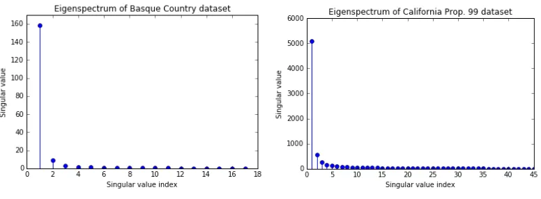
We will also analyze both case studies under a Bayesian setting. From our results, we see that our predictive uncertainty, captured by the standard deviation of the predictive distribution, is influenced by the number of singular values used in the de-noising process. Therefore, we have plotted the eigenspectrum of the two case study datasets below. Clearly, the bulk of the signal contained within the datasets is encoded into the top few singular values – in particular, the top two singular values. Given that the validation errors computed via forward chaining are nearly identical for low-rank settings (with the exception of a rank-1 approximation), we shall use a rank-2 approximation of the data matrix. In order to exhibit the role of thresholding in the interplay between bias and variance, we also plot the cases where we use threshold values that are too high (bias) or too low (variance). For each figure, the dotted blue line will represent our posterior predictive means while the shaded light blue region spans one standard deviation on both sides of the mean. As we shall see, our predictive uncertainty is smallest in the neighborhood around the pre-intervention period. However, the level of uncertainty increases as we deviate from the the intervention point, which appeals to our intuition.

In order to choose an appropriate choice of the prior parameter α, we first use forward-chaining for the ridge regression setting to find the optimal regularization hyperparameterη. By observing the expressions of (19) and (40), we see thatη=ασ2since ridge regression is closely related to MAP estimation for a zero-mean, isotropic Gaussian prior. Consequently, we chooseα=η/σˆ2 whereη is the value obtained via forward chaining.

5.1 Basque Country

(a) Eigenspectrum of Basque data. (b)Eigenspectrum of California data.

Figure 1: Eigenspectrum

for each region were used including demographic information pertaining to one’s educational status, and average shares for six industrial sectors.

Results. Figure 2a shows that our method (for all three estimators) produces a very similar qualitative synthetic control to the original method even though we do not utilize additional predictor variables. Specifically, the synthetic control resembles the observed GDP in the pre-treatment period between 1955-1970. However, due to the large-scale terrorist activity in the mid-70s, there is a noticeable economic divergence between the synthetic and observed trajectories beginning around 1975. This deviation suggests that terrorist activity negatively impacted the economic growth of Basque Country.

One subtle difference between our synthetic control – for the case of linear and ridge regression – and that of Abadie and Gardeazabal (2003) is between 1970-75: our approach suggests that there was a small, but noticeable economic impact starting just prior to 1970, potentially due to first terrorist attack in 1968. Notice, however, that the original synthetic control of Abadie and Gardeazabal (2003) diverges only after 1975. Our LASSO estimator’s trajectory also agrees with that of the original synthetic control method’s, which is intuitive since both estimators seek sparse solutions.

To study the robustness of our approach with respect to missing entries, we discard each data point uniformly at random with probability 1−p. The resulting control for different values ofpis presented in Figure 2b suggesting the robustness of our (linear) algorithm. Finally, we produce Figure 2c by applying our algorithm without the de-noising step. As evident from the Figure, the resulting predictions suffer drastically, reinforcing the value of de-noising. Intuitively, using an appropriate thresholdµequates to selecting the correct model complexity, which helps safeguard the algorithm from potentially overfitting to the training data.

Placebo tests. We begin by applying our robust algorithm to the Spanish region of Cataluna, a control unit that is not only similar to Basque Country, but also exposed to a much lower level of terrorism Abadie et al. (2011). Observing both the synthetic and observed economic evolutions of Cataluna in Figure 3a, we see that there is no identifiable treatment effect, especially compared to the divergence between the synthetic and observed Basque trajectories. We provide the results for the regions of Aragon and Castilla Y Leon in Figures 3b and 3c.

(a) Comparison of methods. (b) Missing data. (c) Impact of de-noising.

Figure 2: Trends in per-capita GDP between Basque Country vs. synthetic Basque Country.

(a)Cataluna. (b)Aragon. (c) Castilla Y Leon.

Figure 3: Trends in per-capita GDP for placebo regions.

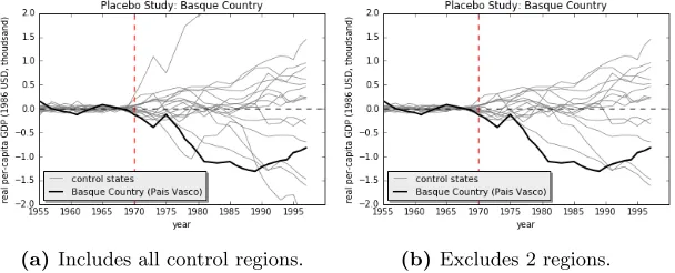
plot helps visualize the extreme post-intervention divergence between the predicted means and the observed values for Basque. Up until about 1990, the divergence for Basque Country is the most extreme compared to all other regions (placebo studies) lending credence to the belief that the effects of terrorism on Basque Country were indeed significant. Refer to Figure 4b for the same test but with Madrid and Balearic Islands excluded, as per Abadie et al. (2011). The conclusions drawn should remain the same, pointing to the robustness of our approach.

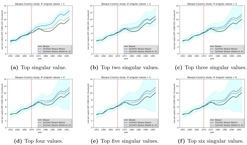
Bayesian approach. We plot the resulting Bayesian estimates in the figures below under varying thresholding conditions. It is interesting to note that our uncertainty grows dramatically once we include more than two singular values in the thresholding process. This confirms what our theoretical

(a) Includes all control regions. (b)Excludes 2 regions.

(a)Top singular value. (b) Top two singular values. (c)Top three singular values.

(d) Top four values. (e)Top five singular values. (f )Top six singular values.

Figure 5: Trends in per-capita GDP between Basque Country vs. synthetic Basque Country.

results indicated earlier: choosing a smaller threshold,µ, would lead to a greater number of singular values retained which results in higher variance. On the other hand, notice that just selecting 1 singular value results in an apparently biased estimate which is overestimating the synthetic control. It appears that selecting the top two singular values balance the bias-variance tradeoff the best and is also agrees with our earlier finding that the data matrix appears to be of rank 2 or 3. Note that in this setting, we would find it hard to reject the null-hypothesis because the observations for the treated unit lie within the uncertainty band of the estimated synthetic control.

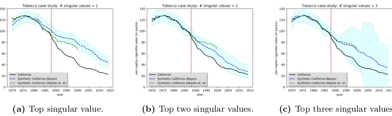
5.2 California Anti-tobacco Legislation

We study the impact of California’s anti-tobacco legislation, Proposition 99, on the per-capita cigarette consumption of California. In 1988, California introduced the first modern-time large-scale anti-tobacco legislation in the United States Abadie et al. (2010). To analyze the effect of California’s anti-tobacco legislation, we use the annual per-capita cigarette consumption at the state-level for all 50 states in the United States, as well as the District of Columbia, from 1970-2015. Similar to the previous case study, Abadie and Gardeazabal (2003) uses 6 additional observable covariates per state, e.g. retail price, beer consumption per capita, and percentage of individuals between ages of 15-24, to predict their synthetic California. Furthermore, Abadie and Gardeazabal (2003) discarded 12 states from the donor pool since some of these states also adopted anti-tobacco legislation programs or raised their state cigarette taxes, and discarded data after the year 2000 since many of the control units had implemented anti-tobacco measures by this point in time.

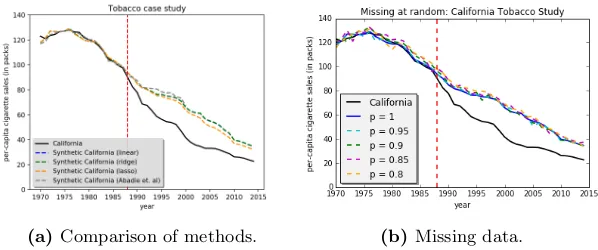
(a) Comparison of methods. (b) Missing data.

Figure 6: Trends in per-capita cigarette sales between California vs. synthetic California.

(a) Colorado. (b)Iowa. (c) Wyoming.

Figure 7: Placebo Study: trends in per-capita cigarette sales for Colorado, Iowa, and Wyoming.

again robust to randomly missing data.

Placebo tests. We now proceed to apply the same placebo tests to the California Prop 99 dataset. Figures 7a, 7b, and 7c are three examples of the applied placebo tests on the remaining states (including District of Columbia) within the United States.

Finally, similar to Abadie et al. (2010), we plot the differences between our estimates and the ac-tual observations for California and all other states, individually, as placebos. Note that Abadie et al. (2010) excluded twelve states but we keep all states. Figure 8a shows the resulting plot for all states with the solid black line being California. This plot helps visualize the extreme post-intervention divergence between the predicted means and the observed values for California. Up until about 1995, the divergence for California was clearly the most significant and consistent outlier compared to all other regions (placebo studies) lending credence to the belief that the effects of Proposition 99 were indeed significant. Refer to Figure 8b for the same test but with the same twelve states excludes as in Abadie et al. (2010). Just like the Basque Country case study, the exclusion of states should not affect the conclusions drawn.

(a)Includes all donors. (b) Excludes 12 states.

Figure 8: Per-capita cigarette sales gaps in California and control regions.

(a)Top singular value. (b)Top two singular values. (c) Top three singular values.

Figure 9: Trends in per-capita cigarette sales between California vs. synthetic California.

effect of Prop. 99, even though the legislation did probably discourage the consumption of cigarettes – a conclusion reached by both our robust approach and the classical approach.

Remark 9 We note that in Abadie et al. (2014), the authors ran two robustness tests to examine the sensitivity of their results (produced via the original synthetic control method) to alterations in the estimated convex weights – recall that the original synthetic control estimator produces a β∗ that lies within the simplex. In particular, the authors first iteratively reproduced a new synthetic West Germany by removing one of the countries that received a positive weight in each iteration, demonstrating that their synthetic model is fairly robust to the exclusion of any particular country with positive weight. Furthermore, Abadie et al. (2014) examined the trade-off between the original method’s ability to produce a good estimate and the sparsity of the given donor pool. In order to examine this tension, the authors restricted their synthetic West Germany to be a convex combination of only four, three, two, and a single control country, respectively, and found that, relative to the baseline synthetic West Germany (composed of five countries), the degradation in their goodness of fit was moderate.

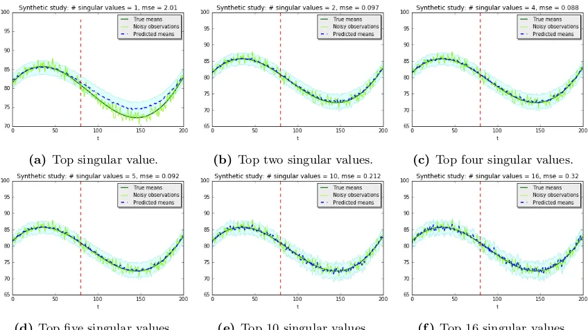
5.3 Synthetic simulations

We conduct synthetic simulations to establish the various properties of the estimates in both the pre-and post-intervention stages.

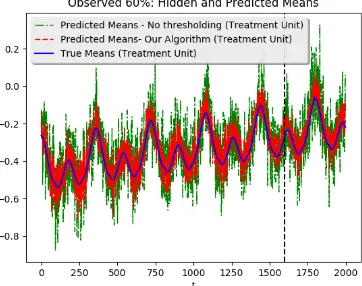
Figure 10: Treatment unit: noisy observations (gray) and true means (blue) and the estimates from our algorithm (red) and one where no singular value thresholding is performed (green). The plots show all entries normalized to lie in range [−1,1]. Notice that the estimates in red generated by our model are much better at estimating the true underlying mean (blue) when compared to an algorithm which performs no singular value thresholding.

Figure 11: Same dataset as shown in Figure 10 but with 40% data missing at random. Treatment unit: not showing the noisy observations for clarity; plotting true means (blue) and the estimates from our algorithm (red) and one where no singular value thresholding is performed (green). The plots show all entries normalized to lie in range [−1,1].

mit=f(θi, ρt). In the experiments described in this section, we use the following: f(θi, ρt) =θi+ (0.3·θi·ρt/T)∗(expρt/T)

+ cos(f1π/180) + 0.5 sin(f2π/180) + 1.5 cos(f3π/180)−0.5 sin(f4∗π/180),

where f1, f2, f3, f4 define the periodicities: f1 =ρtmod (360), f2 =ρtmod (180), f3 = 2·ρtmod (360), f4= 2.0·ρtmod (180). The observed valueXit is produced by adding i.i.d. Gaussian noise to mean with zero mean and varianceσ2_{. For this set of experiments, we useN = 100, T = 2000, while} assuming the treatment was performed att= 1600.

Table 1: Training vs. generalization error

Noise

Training error

Generalization error

3.1

0.48

0.53

2.5

0.31

0.34

1.9

0.19

0.22

1.3

0.09

0.1

0.7

0.027

0.03

0.4

0.008

0.009

0.1

0.0005

0.0006

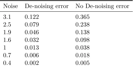
Table 2: Impact of thresholding

Noise

De-noising error

No De-noising error

3.1

0.122

0.365

2.5

0.079

0.238

1.9

0.046

0.138

1.6

0.032

0.098

1

0.013

0.038

0.7

0.006

0.018

0.4

0.002

0.005

pre-intervention MSE for varying noise levels,σ2_{. Thus suggesting efficacy of our algorithm. Figures} 10 and 11 plot the estimates of algorithm with no missing data (Figure 10) and with 40% randomly missing data (Figure 11) on the same underlying dataset. All entries in the plots were normalized to lie within [−1,1]. These plots confirm the robustness of our algorithm. Our algorithm outperforms the algorithm with no singular value thresholding under all proportions of missing data. The estimates from the algorithm which performs no singular value thresholding (green) degrade significantly with missing data while our algorithm remains robust.

Benefits of de-noising. We now analyze the benefit of de-noising the data matrix, which is the main contribution of this work compared to the prior work. Specifically, we study the generalization error of method using de-noising via thresholding and without thresholding as in prior work. The results summarized in Table 2 show that for range of parameters the generalization error with de-noising is consistency better than that without de-noising.