The Thirty-Third AAAI Conference on Artificial Intelligence (AAAI-19)
Active Mini-Batch Sampling Using Repulsive Point Processes
Cheng Zhang,
1Cengiz ¨
Oztireli,
2Stephan Mandt,
3Giampiero Salvi
4 1. Microsoft Research, Cambridge, UK, [email protected] 2. Disney Research, Zurich, Switzerland, [email protected] 3. University of California,Irvine,Los Angeles, USA, [email protected]4. KTH Royal Institute of Technology, Stockholm, Sweden, [email protected]
Abstract
The convergence speed of stochastic gradient descent (SGD) can be improved by actively selecting mini-batches. We ex-plore sampling schemes where similar data points are less likely to be selected in the same mini-batch. In particular, we prove that such repulsive sampling schemes lower the vari-ance of the gradient estimator. This generalizes recent work on using Determinantal Point Processes (DPPs) for mini-batch diversification (Zhang et al., 2017) to the broader class of re-pulsive point processes. We first show that the phenomenon of variance reduction by diversified sampling generalizes in particular to non-stationary point processes. We then show that other point processes may be computationally much more efficient than DPPs. In particular, we propose and investigate Poisson Disk sampling—frequently encountered in the com-puter graphics community—for this task. We show empirically that our approach improves over standard SGD both in terms of convergence speed as well as final model performance.
Introduction
Stochastic gradient descent (SGD) (Bottou 2010) is key to modern scalable machine learning. Combined with back-propagation, it forms the foundation to train deep neural net-works (LeCun et al. 1998b). Applied to variational inference (Hoffman et al. 2013; Zhang et al. 2017a), it enables the use of probabilistic graphical models on massive data. SGD train-ing has contributed to breakthroughs in many applications (Krizhevsky et al. 2012; Mikolov et al. 2013).
A key limitation for the speed of convergence of SGD algorithms is the stochastic gradient noise. Smaller gradient noise allows for larger learning rates and therefore faster convergence. For this reason, variance reduction for SGD is an active research topic.
Several recent works have shown that the variance of SGD can be reduced when diversifying the data points in a mini-batch based on their features (Zhao and Zhang 2014; Fu and Zhang 2017; Zhang et al. 2017b). When data points are coming from similar regions in feature space, their gradi-ent contributions are positively correlated. Diversifying data
Copyright c2019, Association for the Advancement of Artificial Intelligence (www.aaai.org). All rights reserved.
1
This work was initialized when the first author was at Disney Research, and was carried out when the author was at KTH and Microsoft Research. This research was partly supported by the CHIST-ERA project IGLU.
points by sampling from different regions in feature space de-correlates their gradient contributions, which leads to a better gradient estimation.
Another benefit of actively biasing the mini-batch sam-pling procedure relates to better model performance (Chang et al. 2017; Shrivastava et al. 2016; Zhang et al. 2017b). Zhang et al. (2017b) biased the data towards a more uniform distribution, upsampling data-points in scarce regions and downsampling data points in dense regions, leading to a bet-ter performance during test time. Chen and Gupta (2015) showed that training on simple classification tasks first, and later adding more difficult examples, leads to a clear perfor-mance gain compared to training on all examples simultane-ously. We refer to such schemes which modify the marginal probabilities of each selected data point asactive bias. The above results suggest that utilizing an active bias in mini-batch sampling can result in improved performance without additional computational cost.
In this work, we present a framework for active mini-batch sampling based on repulsive point processes. The idea is simple: we specify a data selection mechanism that actively selects a mini-batch based on features of the data. This mech-anism introducesrepulsionbetween the data points, meaning that it suppresses data points with similar features to co-occur in the same mini-batch. We use repulsive point processes for this task. Finally, the chosen mini-batch is used to perform a stochastic gradient step, and this scheme is repeated until convergence.
Our framework generalizes the recently proposed mini-batch diversification based on determinantal point processes (DPP) (Zhang et al. 2017b) to a much broader class of re-pulsive processes, and allows users to encode any preferred active bias with efficient mini-batch sampling algorithms. In more detail, our contributions are as follows:
1. We propose to use point processes for active mini-batch selection.
We provide a theoretical analysis which shows that mini-batch selection with repulsive point processes may reduce the variance of stochastic gradient descent. The proposed approach can accommodate point processes with adaptive densities and adaptive pair-wise correlations. Thus, we can use it for data subsampling with an active bias.
repulsive point processes based on Poisson Disk Sampling (PDS).
We propose PDS with dart throwing for mini-batch selec-tion. Compared to DPPs, this improves the sampling costs fromN k3to merelyk2, whereNis the number of data
points andkis the mini-batch size.
We propose a dart-throwing method with an adaptive disk size and adaptive densities to sample mini-batches with an active bias.
3. We test our proposed method on several machine learning applications from the domains of computer vision and speech recognition. We find increased model performance and faster convergence due to variance reduction.
Related Work
In this section, we begin with reviewing the most relevant work ondiversified mini-batch sampling. Then, we discuss the benefits of subsampling schemes with anactive bias, where data are either reweighed or re-ordered. Finally, we review the relevant aspects ofpoint processes.
Diversified Mini-Batch Sampling Prior research (Zhao and Zhang 2014; Fu and Zhang 2017; Zhang et al. 2017b; Yin et al. 2017) has shown that sampling diversified mini-batches can reduce the variance of stochastic gradients. It is also the key to overcome the problem of the saturation of the convergence speed in the distributed setting (Yin et al. 2017). Diversifying the data is also computationally efficient for large-scale learning problems (Zhao and Zhang 2014; Fu and Zhang 2017; Zhang et al. 2017b). Buchholz et al. (2018) used diversified sampling for optimizing Monte-Carlo objectives in variational inference.
Zhang et al. (2017b) recently proposed to use DPPs for diversified mini-batch sampling and drew the connection to stratified sampling (Zhao and Zhang 2014) and clustering-based preprocessing for SGD (Fu and Zhang 2017). A disad-vantage of the DPP-approach is the computational overhead. Besides presenting a more general theory, we provide more efficient point processes in this work.
Active Bias Different types of active bias in subsampling the data can improve the convergence and lead to improved final performance in model training (Alain et al. 2015; Gopal 2016; Chang et al. 2017; Chen and Gupta 2015; Shrivastava et al. 2016). As summarized in Chang et al. (2017), self-paced learning biases towards easy examples in the early learning phase. Active-learning, on the other hand, puts more emphasis on uncertain cases, and hard example mining focuses on the difficult-to-classify examples.
Chang et al. (2017) investigate a supervised setup and sample data points, which have high prediction variance, more often. (Gopal 2016) (2017) maintain a desired class distribution during batch sampling. Diversified mini-batch sampling with DPPs (Zhang et al. 2017b) re-weights the data towards a more uniform distribution, which improves the final performance when the data set is imbalanced.
The choice of a good active bias depends on the data set and problem at hand. Our proposed method is compatible with different active bias preferences.
Point Processes Point processes have a long history in physics and mathematics, and are heavily used in computer graphics (Macchi 1975; Ripley 1976; Illian et al. 2008;
¨
Oztireli and Gross 2012; Lavancier et al. 2015). DPPs, as a group of point processes, have been introduced and used in the machine learning community in recent years (Kulesza et al. 2012; Li et al. 2015; Kathuria et al. 2016).
Other types of point processes have been less explored and used in machine learning. There are many different re-pulsive point processes, such as PDS, or Gibbs processes, with properties similar to DPPs, but with significantly higher sampling efficiency (Illian et al. 2008). Additionally, more flexible point processes with adaptive densities and interac-tions are well studied in computer graphics (Li et al. 2010; Roveri et al. 2017; Kita and Miyata 2016), but not explored much in the machine learning community. Our proposed framework is based on generic point processes. As one of the most efficient repulsive point processes, we advocate Poisson disk sampling in this paper.
Repulsive Point Processes
for Variance Reduction
In this section, we first briefly introduce our main idea of using point processes for mini-batch sampling in the con-text of the problem setting and revisit point processes. We prove that any repulsive point process can lead to reduced gradient variance in SGD, and discuss the implications of this result. The theoretical analysis in this section leads to multiple practical algorithms.
Problem Setting
Consider a loss function`(x, θ), whereθare the model pa-rameters, andxindicates the data. In this paper, we consider a modified empirical risk minimization problem (Zhang et al. 2017b):
ˆ
J(θ) =Exˆ∼P[`(ˆx, θ)]. (1)
P indicates a point process defining a distribution over sub-setsxˆof the data, which will be specified below. Note that this leads to a potentially biased version of the standard em-pirical risk (Bottou 2010). Debiasing the objective is possible. It requires re-weighting the loss for each data point inverse proportional to its marginal probability to be sampled (Zhang et al. 2017b).
We optimize Eq. 1 via stochastic gradient descent, which leads to the updates
θt+1 =θt−ρtGˆ =θt−ρt|B1|
X
i∈B
∇`(xi, θ), B∼ P.
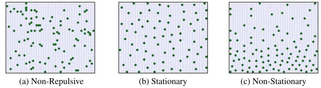
(a) Non-Repulsive (b) Stationary (c) Non-Stationary
Figure 1: Examples of sampling a subset of data points. We sampled different subsets of 100 points (dark green) from a bigger set of points (light blue), using three different point processes. Panel 1(a) shows a uniformly randomly sampled subset. Panel 1(b) and panel 1(c) show two examples with different repulsive point processes.
different mini-batches. Therefore, our scheme generalizes SGD in that the data points in the mini-batchBare selected actively, rather than uniformly.
Figure 1 shows examples of subset selection using different point processes. Drawing the data randomly without replace-ment corresponds to a point process as well, thus standard SGD trivially belongs to the class of algorithms considered here. In this paper, we investigate different point processes and analyze how they improve the performance of different models on empirical data sets.
Background on Point Processes
Point processes are generative processes of collections of points in some measure space (Møller and Waagepetersen 2004; Illian et al. 2008). They can be used to sample subsets of data with various properties, either from continuous spaces or from discrete sets, such as a finite dataset. In this paper, we explore different point processes to sample mini-batches with different statistical properties.
More formally, a point processPinRdcan be defined by
considering the joint probabilities of finding points generated by this process in infinitesimal volumes. One way to express these probabilities is via product densities. Let xi denote some arbitrary points in Rd, and B
i infinitesimal spheres
centered at these points with volumesdxi=|Bi|. Then the
nthorder product density%(n)is defined by
p(x1,· · · ,xn) =%(n)(x1,· · ·,xn)dx1· · ·dxn,
wherep(x1,· · ·,xn)is the joint probability of having a point
of the point processPin each of the infinitesimal spheresBi.
We can usePto generate infinitely many point configurations, each corresponding to e.g. a mini-batch.
For example, DPP defines this probability of sampling a subset as being proportional to the determinant of a kernel matrix. It is thus described by the nth order
prod-uct density (Lavancier et al. 2012): %(n)(x
1,· · ·,xn) =
det[C](x1,· · · ,xn), wheredet[C](x1,· · ·,xn)is the
deter-minant of then×nsized sub-matrix of kernel matrix C with entries specified byx1,· · ·,xn.
For our analysis, we will just need the first and second order product density, which are commonly denoted by λ(x) :=%(1)(x),%(x,y) := %(2)(x,y). An important
spe-cial case of point processes is stationary processes. For such processes, the point distributions generated are translation invariant, where the intensity is a constant.
Point Processes for Active Mini-Batch Sampling
Recently, Zhang et al. (2017b) investigated how to utilize a particular type of point process, DPP, for mini-batch diversifi-cation. Here, we generalize the theoretical results to arbitrary stochastic point processes, and elaborate on how the resulting formulations can be utilized for SGD based algorithms. This opens the door to exploiting a vast literature on the theory of point processes, and efficient algorithms for sampling.SGD-based algorithms utilize the estimator Gˆ(θ) = 1
|B|
P
i∈B∇`(xi, θ)for the gradient of the objective. Each
mini-batch, i.e. set of data points in this estimator, can be con-sidered as an instance of an underlying point processP. Our goal is to design sampling algorithms for improved learning performance by altering the bias and variance of this gradient estimator.
We first derive a closed form formula for the variance
varP( ˆG)of the gradient estimator for general point
pro-cesses. We then show that, under mild regularity assumptions, repulsive point processes generally imply variance reduction. For what follows, letg(x, θ) =∇`(x, θ)denote the gradient of the loss function, and recall thatk=|B|, the mini-batch size.
Theorem 1. The variancevarP( ˆG)of the gradient estimate
ˆ
Gin SGD for a general stochastic point processPis given by:
varP( ˆG) =
1
k2
Z
V×V
λ(x)λ(y)g(x, θ)Tg(y, θ) (2)
%(x,y)
λ(x)λ(y)−1
dxdy
+ 1
k2
Z
V
kg(x, θ)k2λ(x)dx.
Proof. In Appendix.
Remark 2. For standard SGD, we have %(x,y) =
λ(x)λ(y). This is due to the nature of random sampling, where sampling a point is independent of already sampled points. Note that this applies also to adaptive sampling with non-constantλ(x). Hence, the term[λ%(x)(xλ,y)(y)−1]vanishes in SGD. In contrast, we show next that this term may induce a variance reduction for repulsive point processes.
Remark 3. Repulsive point processes may make the first term in Eq. 2 negative, implying variance reduction. For re-pulsive point processes, the probability of sampling points that are close to each other is low. Consequently, ifxandy
are close,%(x,y)< λ(x)λ(y), and the term[λ%(x)(xλ,y)(y)−1]
is negative. This is due to points repelling each other (we will elaborate more on this in the next section). Furthermore, assuming that the loss function is sufficiently smooth in its data argument, the gradients are aligned for close points i.eg(x, θ)Tg(y, θ)>0. This combined implies that close
points provide negative contributions to the first integral in Eq. 2. The contributions of points farther apart average out and become negligible due to gradients not being correlated with%(x,y), which is the case for all current sampling al-gorithms and the ones we propose in the next section. The negative first term in Eq. 2 leads to variance reduction, for repulsive point processes.
Implications. This proposed theory allows us to use any point process for mini-batch sampling, such as DPP, finite Gibbs processes, Poisson disk sampling (PDS), and many more (Illian et al. 2008). It thus offers many new directions of possible improvement. Foremost, we can choose point processes with a different degree of repulsion (Biscio et al. 2016), and computational efficiency. Furthermore, in this general theory, we are able to adapt the density and alter the pair-wise interactions to encode our preference. In the next section, we propose several practical algorithms utilizing these benefits.
Poisson Disk Sampling
for Active Mini-batch Sampling
We adapt efficient dart throwing algorithms for fast repul-sive and adaptive mini-batch sampling. We further extend the algorithm with an adaptive disk size and density. For su-pervised setups, we shrink the disc size towards the decision boundary, using mingling indices (Illian et al. 2008). This biases towards hard examples and improves classification accuracy.
Stationary Poisson Disk Sampling
PDS is one type of repulsive point process. It demonstrates stronger local repulsion compared to DPP (Biscio et al. 2016). Typically, it is implemented with the efficient dart throwing algorithm (Lagae and Dutr´e 2008), and provides similar point arrangements to DPP, albeit much more efficiently.
This process dictates that the smallest distance between each pair of sample points should be at leastrwith respect to some distance measureD. The second order product density
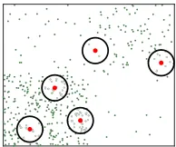
Figure 2: Demonstration of PDS. The black circles of a cer-tain radiusrmark regions claimed by the collected points (red). For the next iteration, if the newly sampled point falls in any of the circles (points colored in gray), this point will be rejected.
%(x, y)for PDS is zero when the distance between two points are smaller than the disk radius||x−y|| ≤r, and converges to%(x, y) =λ(x)λ(y)when the two points are far ( ¨Oztireli
and Gross 2012). Thus,hλ%(x)(xλ,y)(y)−1i=−1<0when the points are within distancer, and0when they are far.
As demonstrated in Figure 2, the basic dart throwing algo-rithm for PDS works as follows in each iteration: 1) randomly sample a data point; 2) if it is within a distancerof any al-ready accepted data point, reject; otherwise, accept the new point. We can also specify the maximum sampling size k. This means that we terminate the algorithm whenkpoints have been accepted. The computational complexity of PDS with dart throwing2isO(k2). This is much lower than the
complexityO(N k3)for k-DPP, whereNis the number of
data points in the dataset. In the rest of the paper, we refer to this version of PDS as“Vanilla PDS”.
Poisson Disk Sampling with Adaptive Density
To further utilize the potential benefit of our framework, we propose several variations of PDS. In particular, we use min-gling index based marked processes. We then propose three variants as explained below: Easy PDS, where only the points far from decision boundaries repulse each other, as well as Dense PDS and Anneal PDS, where we can impose prefer-ences on point densities.
Mingling Index The mingling indexM¯K(xi)is defined as
(Illian et al. 2008):
¯
MK(xi) =
1
K
K
X
j=1
1 m(xi)6=m(xj)
, (3)
wherem(xi)indicates the mark of the pointxi. In case of
a classification task, the mark is the class label.M¯K(xi)is
the ratio of points with different marks thanxiamong itsK
nearest neighbors.
Depending on the mingling index, there are three different situations. Firstly, ifM¯K(xi) = 0, the region aroundxionly
2
Algorithm 1Draw throwing for Dense PDS
Input:datax, mini-batch sizeS, mingling indexMfor all data, the parameter for categorical distribution to sample mingling indexπ, disk radiusr0
repeat
sample a mingling indexm∼Cat(π)
randomly sample a pointiwith mingling indexm if xiis not in disk of any samplesthen
insertxitoB
end if
untilSpoints have been accepted for the mini-batch
includes points from the same class. This makesxia
rela-tively easy point to classify. This type of points is preferred to be sampled in the early iterations for self-paced learning. Secondly, ifM¯K(xi)>0, this point may be close to a
de-cision boundary. For variance reduction, we do not need to repulse this type of points. Additionally, sampling this type of points more often may help the model to refine the deci-sion boundaries. Finally, ifM¯K(xi)is very high, the point
is more likely to be a hard negative. In this case, the point is mostly surrounded by points from other classes. On a side note, points with high mingling indices can be interpreted as support vectors (Cortes and Vapnik 1995).
Adaptive Variants of Poisson Disk Sampling Gradients may change drastically when points are close to decision boundaries. Points in this region, thus, violate the assumption in Remark 3. Because of this, our first simple extension, which we call“Easy PDS”, sets the disk radius tor0when
the point has a mingling indexMxi = 0, and to0ifMxi>0. This means that only easy points (withMxi = 0) repulse. On average, “Easy PDS” is expected to sample more of the difficult points compared with “Vanilla PDS”.
For many tasks, when the data is highly structured, there are only few data points that are close to the decision bound-ary. To refine the decision boundary, inspired by hard ex-ample mining, we can sex-ample points with a high mingling index more often. We thus propose the“Dense PDS”method summarized in Algorithm 1. Instead of drawing darts ran-domly, we draw darts based on different mingling indices. The mingling indices can assumeK+ 1values, whereK is the number of nearest neighbors. We thus can specify a parameterπfor a categorical distribution to sample mingling indices first. Then we randomly sample a dart which has the given mingling index. In this way, we can encode our preferred density with respect to the mingling index.
It is straightforward to introduce an annealing mechanism in “Dense PDS” by using a differentπnat each iterationn.
Inspired by self-paced learning, we can give higher density to points with low mingling index in the early iterations, and slowly increase the density of points with high mingling index. We refer this method as“Anneal PDS”.
Note that all our proposed sampling methods only rely on the properties of the given data instead of any model parameters. Thus, they can be easily used as a pre-processing step, prior to the training procedure of the specific model.
Experiments
We evaluate the performance of the proposed method in vari-ous application scenarios. Our methods show clear improve-ments compared to baseline methods in each case. We first demonstrate the behavior of different varieties of our method using a synthetic dataset. Secondly, we compare Vanilla PDS with DPP as in (Zhang et al. 2017b) on the Oxford flower classification task. Finally, we evaluate our proposed methods with two different tasks with very different properties: image classification with MNIST, and speech command recognition.
Synthetic Data We evaluate our methods on two-dimensional synthetic datasets to illustrate the behavior of different sampling strategies. Figure 3 shows two classes (green and red dots) separated by a wave-shaped (sine curve) decision boundary (yellow line). Intuitively, it should be fa-vorable to sample diverse subsets and even more beneficial to give more weight to the data points at the decision boundary, i.e., sampling them more often. We sample one mini-batch with batch size30 using different sampling methods. For each method, we train a neural network classifier with one hidden layer of five units, using a single mini-batch. This model, albeit simple, is sufficient to handle the non-linear decision boundary in the example.
Figure 3 shows the decision boundaries by repeating the ex-periment 30 times. In order to illustrate the sampling schemes, we also show one example of sampled mini-batch using blue dots. In the random sampling case (Figure 3(a)), we can see that the mini-batch is not a good representation of the original dataset as some random regions are more densely or sparsely sampled. Consequently, the learned decision boundary is very different from the ground truth. Figures 3(b) shows Vanilla PDS. Because of the repulsive effect, the sampled points cover the data space more uniformly and the decision bound-ary is improved compared to Figure 3(a). In Figure 3(c), we used Easy PDS, where the disk radius adapts with the min-gling index of the points. We can see that points close to the decision boundary do not repel each other. This leads to a potentially more refined decision boundary as compared to Figure 3(b). Finally, Dense PDS, shown in Figure 3(d), chooses more samples close to the boundary and leads to the most precise decision boundary with a single mini-batch.
Moreover, to demonstrate the scalibilty of PDS, we gener-ate synthetic datasets with different dataset sizes and sample mini-batches using PDS. We report the sampling time in Ta-ble 1. We can see that the sampling time for a mini-batch using PDS is stable across different dataset sizesNand only differs with respect to mini-batch sizek. More experiments on variance reduction are shown in the appendix.
(a) Random (b) Vanilla PDS (c) Easy PDS (d) Dense PDS
Figure 3: Comparison of performance using one mini-batch sample distribution on synthetic data. Each experiment is repeated 30 times. The resulting decision boundaries are drawn as transparent black lines and the ground truth decision boundary is shown in yellow. As an example, the points from one of the sampled mini-batches are shown in blue.
N: 4096 N: 8192 N: 16384 N: 32768 N: 65536 N: 131072 N: 262144 N: 524288 N: 1048576
k=50 0.0066 0.0064 0.0064 0.0061 0.0062 0.0069 0.0063 0.0060 0.0061 k=100 0.0239 0.0237 0.0235 0.0234 0.0227 0.0225 0.0228 0.0239 0.0262
Table 1: Average CPU time (sec) to sample each mini-batch using PDS.Nis the number of data andkis the mini-batch size. The table confirms that the computational complexity of PDS isO(k2), which does not depend on the dataset sizeN, as opposed
toO(N k3)for k-DPP. Thus, PDS is able to scale to massive datasets with large mini-batches. Note that, vanilla PDS is used
here, however, other variants of PDS have the same computational complexity for sampling but may have some pre-processing overhead such as computation of mingling index.
100 101 102
Num of Epochs 0.2
0.4 0.6 0.8
Test Accuracy PDS DPP Baseline
(a) k=80
100 101 102
Num of Epochs 0.2
0.4 0.6 0.8
Test Accuracy PDS DPP Baseline
(b) k=150
Figure 4: Oxford Flower Classification with Softmax. PDS has similar performance as DPP for sampling mini-batches. However PDS is more efficient as Table 2 shows. Both meth-ods converges faster than traditional SGD (Baseline).
using DPP, PDS demonstrates significant improvement on sampling efficiency as shown in Table 2. More experimental results with different settings are presented in the appendix.
MNIST We further show results for hand-written digit clas-sification on the MNIST dataset (LeCun et al. 1998a). We compare different variations of our method with two base-lines: the traditional SGD and ActiveBias (Chang et al. 2017). We use half of the training data and the full test data. As detailed in the appendix, with MNIST, data are well clustered and most data points have mingling index0(easy to classify). A standard multi-layer convolutional neural network (CNN)
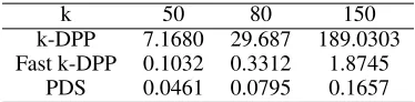
k 50 80 150
k-DPP 7.1680 29.687 189.0303 Fast k-DPP 0.1032 0.3312 1.8745
PDS 0.0461 0.0795 0.1657
Table 2: CPU time (sec) to sample one mini-batch. The disk radius ris set to half of the median value of the distance measureDfor PDS.
from Tensorflow3 is used in this experiment with standard
experimental settings (details in appendix).
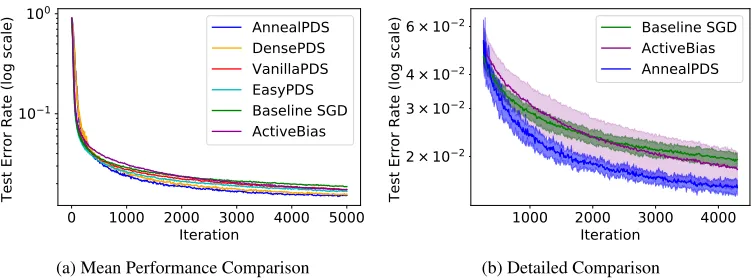
Figure 5(a) shows the test error rate evaluated after each SGD training iteration for different mini-batch sampling methods. All active sampling methods with PDS lead to improved final performance compared to traditional SGD. Vanilla PDS clearly outperforms the baseline method. Easy PDS, performs very similarly to Vanilla PDS with slightly faster convergence in the early iterations. Dense PDS leads to better final performance at the cost of a slight decrease in initial convergence speed. The decision boundary is re-fined because we prefer non-trivial points during training. Anneal PDS further improves Dense PDS with accelerated convergence in the early iterations. Figure 5(b) shows the performance of test accuracy for Anneal PDS compared with baseline methods in a zoomed view.
We thus conclude that all different variations of PDS obtain better final performance, or conversely, achieve the baseline
3
0
1000 2000 3000 4000 5000
Iteration
10
110
0Test Error Rate (log scale)
AnnealPDS
DensePDS
VanillaPDS
EasyPDS
Baseline SGD
ActiveBias
(a) Mean Performance Comparison
1000 2000 3000 4000
Iteration
2 × 10
23 × 10
24 × 10
26 × 10
2Test Error Rate (log scale)
Baseline SGD
ActiveBias
AnnealPDS
(b) Detailed Comparison
Figure 5: MNIST experiment (10 repetitions). The mean performance for each method is reported in Panel (a). We compared all variations of our proposed methods with two baselines: Baseline SGD and ActiveBias (Chang et al. 2017). All our methods perform better than the baselines. AnnealPDS performs best. For better visualization, Panel (b) shows the mean and standard deviation of our proposed Anneal PDS comparing with two baselines closely.
0
500
1000
1500
Iteration
0.2
0.4
0.6
0.8
Validation Error Rate
Dense PDS
Easy PDS
Vannila PDS
Baseline SGD
ActiveBias
Figure 6: Speech experiment (10 repetitions). We compare the performance over the validation set of different variations of PDS with traditional SGD for every 50 iterations. Means and standard deviations are shown.
performance with fewer iterations. With a proper annealing schedule to resemble self-paced learning, we can obtain even more improvement in the final performance.
Speech Command Recognition In this section, we evalu-ate our method on a speech command classification task as described in (Sainath and Parada 2015). The classification task includes twelve classes: ten isolated command words, silence, or unknown class.
The database consists of 64,727 one-second-long audio recordings. As in Sainath and Parada (2015), for each record-ing, 40 MFCC features (Davis and Mermelstein 1980) are extracted at 10 msec time intervals resulting in40×98 fea-tures. We use the TensorFlow implementation4with standard
settings (see appendix). Differently from the MNIST dataset, word classes are not clearly separated and data with different mingling index values are well distributed (see appendix).
Figure 6 shows the accuracy on the validation set evaluated every 50 training iterations. Using Vanilla PDS, the model converges with fewer iterations compared to the traditional
4
https://www.tensorflow.org/tutorials/audio recognition
random sampling of mini-batches. Easy PDS and Dense PDS show similar improvement since few data have0mingling indices in this dataset.
As compared to the MNIST experiment, the gain of Vanilla PDS and Easy PDS is larger in this case since the dataset is more challenging. On the other hand, encouraging more difficult samples has a stronger impact on the MNIST dataset than in the Speech experiment. In all different settings, our mini-batch sampling methods are beneficial for both fast convergence and final model performance.
Discussion
In this work, we propose the use of repulsive point processes for active mini-batch sampling. We provide both theoretical and experimental evidence that using repulsive stochastic point processes can reduce the variance of stochastic gra-dient estimates, which leads to faster convergence. Addi-tionally, our general framework also allows adaptive density and adaptive pair-wise interactions. This leads to further im-provements in model performance thanks to balancing the information provided by the input samples, or enhancing the information around decision boundaries.
Our work is mainly focused on similarity measures in input space, which makes the algorithms efficient without additional run-time costs for learning. In future work, we will explore the use of our framework in the gradient space directly. This can potentially lead to even greater variance reduction. we believe that our proposed method may show even greater advantages in the two-stage framework such as Faster-R-CNN (Ren et al. 2015). Here, point processes can be used for region proposal sampling.
References
Alain, G.; Lamb, A.; Sankar, C.; Courville, A.; and Bengio, Y. 2015. Variance reduction in SGD by distributed importance sampling.arXiv preprint arXiv:1511.06481.
Biscio, C. A. N.; Lavancier, F.; et al. 2016. Quantifying repulsiveness of determinantal point processes. Bernoulli.
Bottou, L. 2010. Large-scale machine learning with stochas-tic gradient descent. InCOMPSTAT. 177–186.
Buchholz, A.; Wenzel, F.; and Mandt, S. 2018. Quasi-Monte Carlo Variational Inference. InICML.
Chang, H.-S.; Learned-Miller, E.; and McCallum, A. 2017. Active bias: Training a more accurate neural network by emphasizing high variance samples. arXiv preprint arXiv:1704.07433.
Chen, X., and Gupta, A. 2015. Webly supervised learning of convolutional networks. InICCV.
Cortes, C., and Vapnik, V. 1995. Support-vector networks. Machine learning.
Davis, S. B., and Mermelstein, P. 1980. Comparison of para-metric representations for monosyllabic word recognition in continuously spoken sentences. IEEE Transactions on Acoustics, Speech, and Signal Processing28(4):357–366. Fu, T., and Zhang, Z. 2017. CPSG-MCMC: Clustering-based preprocessing method for stochastic gradient MCMC. In AISTATS.
Gopal, S. 2016. Adaptive sampling for SGD by exploiting side information. InICML.
Hoffman, M. D.; Blei, D. M.; Wang, C.; and Paisley, J. 2013. Stochastic variational inference.JMLR.
Illian, J.; Penttinen, A.; Stoyan, H.; and Stoyan, D. 2008. Statistical analysis and modelling of spatial point patterns, volume 70. John Wiley & Sons.
Kathuria, T.; Deshpande, A.; and Kohli, P. 2016. Batched gaussian process bandit optimization via determinantal point processes. InNIPS, 4206–4214.
Kita, N., and Miyata, K. 2016. Multi-class anisotropic blue noise sampling for discrete element pattern generation.The Visual Computer.
Krizhevsky, A.; Sutskever, I.; and Hinton, G. E. 2012. Ima-genet classification with deep convolutional neural networks. InNIPS.
Kulesza, A.; Taskar, B.; et al. 2012. Determinantal point processes for machine learning.Foundations and TrendsR
in Machine Learning5(2–3):123–286.
Lagae, A., and Dutr´e, P. 2008. A comparison of methods for generating poisson disk distributions. InComputer Graphics Forum, volume 27, 114–129. Wiley Online Library. Lavancier, F.; Møller, J.; and Rubak, E. H. 2012. Statistical aspects of determinantal point processes. Technical report, Department of Mathematical Sciences, Aalborg University.
Lavancier, F.; Møller, J.; and Rubak, E. 2015. Determinantal point process models and statistical inference. Journal of the Royal Statistical Society: Series B (Statistical Methodology).
LeCun, Y.; Bottou, L.; Bengio, Y.; and Haffner, P. 1998a. Gradient-based learning applied to document recognition. Proceedings of the IEEE86(11):2278–2324.
LeCun, Y.; Bottou, L.; Orr, G. B.; and M¨uller, K.-R. 1998b. Efficient backprop. InNeural networks: Tricks of the trade. Springer. 9–50.
Li, H.; Wei, L.-Y.; Sander, P. V.; and Fu, C.-W. 2010. Anisotropic blue noise sampling. InACM TOG.
Li, C.; Jegelka, S.; and Sra, S. 2015. Efficient sam-pling for k-determinantal point processes. arXiv preprint arXiv:1509.01618.
Macchi, O. 1975. The coincidence approach to stochastic point processes. Advances in Applied Probability.
Mikolov, T.; Chen, K.; Corrado, G.; and Dean, J. 2013. Efficient estimation of word representations in vector space. arXiv preprint arXiv:1301.3781.
Møller, J., and Waagepetersen, R. P. 2004. Statistical infer-ence and simulation for spatial point processes. Chapman & Hall/CRC, 2003.
¨
Oztireli, A. C., and Gross, M. 2012. Analysis and synthesis of point distributions based on pair correlation. ACM Trans. Graph.
Ren, S.; He, K.; Girshick, R.; and Sun, J. 2015. Faster R-CNN: Towards real-time object detection with region pro-posal networks. InNIPS.
Ripley, B. D. 1976. The second-order analysis of stationary point processes. Journal of applied probability.
Roveri, R.; ¨Oztireli, A. C.; and Gross, M. 2017. General point sampling with adaptive density and correlations. Euro-graphics.
Sainath, T. N., and Parada, C. 2015. Convolutional neural net-works for small-footprint keyword spotting. InInterspeech. Shrivastava, A.; Gupta, A.; and Girshick, R. 2016. Train-ing region-based object detectors with online hard example mining. InCVPR.
Yin, D.; Pananjady, A.; Lam, M.; Papailiopoulos, D.; Ram-chandran, K.; and Bartlett, P. 2017. Gradient diversity: a key ingredient for scalable distributed learning. InNIPS WS. Zhang, C.; B¨utepage, J.; Kjellstr¨om, H.; and Mandt, S. 2017a. Advances in variational inference. arXiv preprint arXiv:1711.05597.
Zhang, C.; Kjellstr¨om, H.; and Mandt, S. 2017b. Deter-minantal point processes for mini-batch diversification. In UAI.