Decentralized Dictionary Learning Over Time-Varying
Digraphs
Amir Daneshmand [email protected]
Ying Sun [email protected]
Gesualdo Scutari [email protected]
School of Industrial Engineering Purdue University
West-Lafayette, IN, USA
Francisco Facchinei [email protected]
Department of Computer, Control, and Management Engineering University of Rome “La Sapienza”
Rome, Italy
Brian M. Sadler [email protected]
U.S. Army Research Laboratory Adelphi, MD, USA
Editor:Sathiya Keerthi
Abstract
This paper studies Dictionary Learning problems wherein the learning task is distributed over a multi-agent network, modeled as a time-varying directed graph. This formulation is relevant, for instance, in Big Data scenarios where massive amounts of data are col-lected/stored in different locations (e.g., sensors, clouds) and aggregating and/or process-ing all data in a fusion center might be inefficient or unfeasible, due to resource limitations, communication overheads or privacy issues. We develop a unified decentralized algorithmic framework for this class ofnonconvex problems, which is proved to converge to stationary solutions at a sublinear rate. The new method hinges on Successive Convex Approximation techniques, coupled with a decentralized tracking mechanism aiming at locally estimating the gradient of the smooth part of the sum-utility. To the best of our knowledge, this is the first provably convergent decentralized algorithm for Dictionary Learning and, more generally, bi-convex problems over (time-varying) (di)graphs.
Keywords: Decentralized algorithms, dictionary learning, directed graph, non-convex optimization, time-varying network
1. Introduction and Motivation
This paper introduces, analyzes, and tests numerically the first provably convergent dis-tributed method for a fairly general class of Dictionary Learning (DL) problems. More specifically, we study the problem of finding a matrix D ∈ RM×K (a.k.a. the dictionary),
by which the data matrixS∈RM×N can be represented through a matrixX∈
RK×N, with
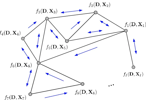
a favorable structure onDandX(e.g., sparsity). We target scenarios where computational resources and data are not centrally available, but distributed over a group of I agents, which can communicate through a (possibly) time-varying, directed network; see Fig. 1.
c
Figure 1: Directed network topology
Each agenti∈ {1,2, . . . , I} owns one block Si ∈RM×ni of the data S ,[S
1, . . . ,SI], with
PI
i=1ni = N. Partitioning the representation matrix X , [X1, . . . ,XI] according to S, withXi ∈RK×ni, the class ofdistributed DL problems we aim at studying reads
min
D,{Xi}Ii=1
U(D,U),
I
X
i=1
fi(D,Xi)
| {z }
,F(D,X) +
I
X
i=1
gi(Xi) +G(D)
s.t. D∈ D, Xi∈ Xi, i= 1, . . . , I,
(P)
where fi : D × Xi → R is the fidelity function of agent i, which measures the mismatch
between the data Si and the (local) model; this function is assumed to be smooth and biconvex (i.e., convex in D for fixed Xi, and vice versa); G:D → R and gi :Xi → R are
(possibly non-smooth) convex functions, which are generally used to impose extra structure on the solution (e.g., low-rank or sparsity); andD ⊆RM×KandX
i ⊆RK×ni are some closed
convex sets. To avoid scaling ambiguity in the model,Dis assumed to be bounded, without loss of generality. Since all fi’s share the common variable D, we call it a shared variable and, by the same token, Xi’s are termed private variables. Note that, in this distributed setting, agentiknows only its own functionsfi(andgi) but notPj6=ifj. Hence, agents aim to cooperatively solve Problem P leveraging local communications with their neighbors.
(Jiang et al., 2011). More details on explicit customizations of the general model P can be found in Sec. 2.
Our distributed setting is motivated by several data-intensive applications in several fields, including signal processing and machine learning, and network systems (such as clouds, cluster computers, networks of sensor vehicles, or autonomous robots) wherein the sheer volume and spatial/temporal disparity of scattered data, energy constraints, and/or privacy issues, render centralized processing and storage infeasible or inefficient. Also, time-varying communications arise, for instance, in mobile wireless networks (e.g., ad-hoc networks), wherein nodes are mobile and/or communicate through fading channels. More-over, since nodes generally transmit at different power and/or communication channels are not symmetric, directed links are a natural assumption.
Our goal is to design a provably convergent decentralized method for Problem P, over
time-varying and directed graphs. To the best of our knowledge this is an open problem, as documented next.
1.1. Challenges and related works
The design of distributed algorithms for P faces the following challenges:
(i) Problem P is non-convex andnon-separable in the optimization variables;
(ii) Each agent iowns exclusivelySi and thus can only compute its own functionfi;
(iii) Each fi depends on a common set of variables−the dictionary D−shared among all the agents, as well as the private variablesXi. Shared and private variables need to be treated differently. In fact, in several applications, the size of private variables is much larger than that of the shared ones; hence, broadcasting agents’ private variables over the network would result in an unaffordable communication overhead;
(iv) The gradient of each fi is in general neither bounded nor globally Lipschitz on the feasible region. This represents a challenge in the design of provably convergent dis-tributed algorithms, as boundedness and Lipschitzianity of the gradient are standard assumptions in the analysis of most distributed schemes for nonconvex problems;
(v) Gand gi’s are nonsmooth;
(vi) The graph is directed, time-varying; no other structure is assumed (such as star or ring topology, etc.), but some long term connectivity properties (cf. Assumption B).
Centralized methods for the solution of Problem P (or some closely related variants) have been extensively studied and prominent examples are (Aharon et al., 2006; Mairal et al., 2010; Razaviyayn et al., 2014b). However, we are not aware of any distributed algorithm that can address challenges i)-vi) (even some subsets of them), as documented next.
theoretical convergence remains an open question, and numerical results are contradictory. For instance, some schemes are shown not to converge while some others fail to reach asymptotic agreement among the local copies of the dictionary; see, e.g. (Chainais and Richard, 2013).
Recently and independently from our conference work (Daneshmand et al., 2016), Zhao et al. (2016) proposed a distributed primal-dual-based method for a class of dictionary learn-ing problems related, but different from Problem P. Specifically, they considered: quadratic loss functions fi, with a quadratic regularization on the dictionary (i.e.,G= 0), and norm ball constraints on the private variables. The network is modeled as a fixed undirected graph. Asymptotic convergence of the scheme to stationary solutions is proved, but no rate analysis is reported. We remark that the scheme in (Zhao et al., 2016), in order to establish convergence, requires some penalty parameters to go to infinity, which makes the method numerically not attractive.
Distributed nonconvex optimization: Since the DL problem P is an instance of non-convex optimization problems, we briefly discuss here the few works in the literature on distributed methods for non-convex optimization (Bianchi and Jakubowicz, 2013; Tatarenko and Touri, 2017; Wai et al., 2017; Di Lorenzo and Scutari, 2016; Sun et al., 2016; Hong et al., 2017; Scutari and Sun, 2019); we group these papers as follows. The schemes in (Bianchi and Jakubowicz, 2013; Tatarenko and Touri, 2017; Wai et al., 2017; Hong et al., 2017), while substantially different, are all applicable tosmooth, unconstrainedoptimization, with (Bianchi and Jakubowicz, 2013; Wai et al., 2017) handling also compact constraints and (Tatarenko and Touri, 2017) implementable on (time-varying) digraphs. The distributed algorithms in (Di Lorenzo and Scutari, 2016; Sun et al., 2016; Scutari and Sun, 2019) can handle objectives with additivenonsmoothconvex functions, with (Sun et al., 2016; Scutari and Sun, 2019) applicable to (time-varying) digraphs.
All the above schemes cannot adequately deal withprivate (i.e.,Xi’s)and shared vari-ables (i.e., D), which are a key feature of Problem P. Furthermore, convergence therein is proved under the assumption that the gradient of (the smooth part of) the objective function is globally Lipschitz continuous, a property that we do not assume and that is not satisfied in many of the applications we consider. The design of provably convergent distributed algorithms for P remains an open problem, let alone rate guarantees.
1.2. Major contributions
In this paper, we propose the first provably convergent distributed algorithm for the gen-eral class of DL problems P, addressing all challenges i)-vi). The proposed approach uses a general convexification-decomposition technique that hinges on recent (centralized) Suc-cessive Convex Approximation methods (Scutari et al., 2014; Facchinei et al., 2015). This technique is coupled with a perturbed push-sum consensus scheme preserving thefeasibility
of the iterates and a tracking mechanism aiming at estimating locally the gradient ofP
putting forth a new non-trivial convergence analysis that, for the first time, i) avoids the as-sumption that the gradients∇fiare globally Lipschitz; and ii) deals withprivateand shared optimization variables. Numerical experiments show that the proposed schemes compare favorably with ad-hoc algorithms, proposed for special instances of Problem P.
1.3. Paper Organization
The rest of the paper is organized as follows. The problem and network setting are intro-duced in Sec. 2, along with some motivating applications. Sec. 3 presents the algorithm and its convergence properties; the proofs of our results are given in the Appendix, Sec. A. Extensive numerical experiments showing the effectiveness of the proposed scheme are dis-cussed in Sec. 5 whereas Sec. 6 draws some conclusions.
1.4. Notation
Throughout the paper we use the following notation. We denote by Rn+ and N+ the non-negative orthant and the set of non-non-negative integers, respectively. Given x ∈ R, dxe
(resp. bxc) denotes the smallest (resp. the largest) integer greater (resp. smaller) than or equal to x. Vectors are denoted by bold lower-case letters (e.g., x) whereas matrices are denoted by bold capital letters (e.g., A). The k-th canonical vector is denoted by ek. The inner product between two real matrices, A and B, is denoted by hA,Bi,tr(A|B), where tr(•) is the trace operator; A⊗B denotes the Kronecker product. Given the real matrix A, with ij-entries denoted by Aij, we will use the following matrix norms: the
Frobenius norm ||A||F ,
q P
i,j|Aij|2; the L1,1 norm ||A||1,1 ,
P
i,j|Aij|; the L2,∞ norm
||A||2,∞ ,maxi
q P
jA2ij; the L∞,∞ norm ||A||∞,∞ = maxi,j|Aij|; and the spectral norm
||A||2 ,σmax(A), where σmax(A) denotes the maximum singular value of A. The matrix quantities ∇Dfi(D,Xi) and ∇Xifi(D,Xi) are the gradients of fi with respect to D and
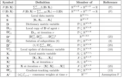
Xi, evaluated at (D,Xi), respectively, with the partial derivatives arranged according to the patterns of D and Xi, respectively. The same convention is adopted for subgradients of gi and G, that are therefore written as matrices of the same dimensions of Xi and D, respectively. Table 1 summarizes the main notation and symbols used in the paper.
Because of the nonconvexity of Problem P, we aim at computing stationary solutions of P, defined as follows: a tuple (D∗,X∗), withX∗ ,[X∗1, . . . ,X∗I] is a stationarity solution of P if the following holds: D∗ ∈ D,X∗i ∈ Xi,i= 1, . . . , I, and
D
∇DF(D∗,X∗),D−D∗E+G(D)−G(D∗) ≥ 0, ∀D∈ D,
h∇Xifi(D ∗
,X∗i),Xi−X∗ii+gi(Xi)−gi(X∗i) ≥ 0, ∀Xi∈ Xi, i= 1, . . . , I.
(2)
2. Problem Setup and Motivating Examples
Symbol Definition Member of Reference
F(D,X) PI
i=1fi(D,Xi) RM×K×RK×N→R (P) U(D,X) F(D,X) +PI
i=1gi(Xi) +G(D) R
M×K×
RK×N→R (P)
Si Local data matrix RM×ni
S [S1,S2, . . . ,SI] RM×N
D Dictionary matrix variable D ⊆RM×K
D(i) Local copy ofDof agenti D ⊆RM×K
Dν(i) D(i) at iterationν D ⊆RM×K
Dν [Dν(1)|,Dν(2)|, . . . ,Dν(I|)]| RM×KI (25)
e
Dν(i) Solution of subproblem (8) D ⊆R
M×K
(8)
Dν (1/I)PIi=1D
ν
(i) D ⊆R
M×K
(25) Uν(i) Local update of dictionary variable D ⊆RM×K (10)
Xi Local matrix variable Xi⊆RK×ni
X [X1,X2, . . . ,XI] X ⊆RK×N
Xν
i Xiat iterationν Xi⊆RK×ni
Xν Xat iterationν: [Xν1,X2ν, . . . ,XνI] X ⊆RK×N (25)
Θν(i) Gradient-tracking variable D ⊆RM×K (13)
Aν (aν
ij)Ii,j=1−consensus weights at timeν RI
×I Assumption F
Table 1: Table of notation
2.1. Problem Assumptions
We consider Problem P under the following assumptions.
Assumption A (On Problem P)
(A1) Each fi :O × Oi →Ris C2, lower bounded, and biconvex, where O ⊇ D andOi ⊇ Xi are convex open sets;
(A2) GivenD∈ D, each∇Xifi(D,•)is Lipschitz continuous onXi, with Lipschitz constant
L∇Xi(D). Furthermore, each L∇Xi :D →R+ is continuous;
(A3) D is compact and convex; and eachXi is closed and convex (not necessarily bounded);
(A4) G:O →R is convex (possibly non-smooth);
(A5) For all i = 1, . . . , I, either i) Xi is compact and gi : Oi → R is convex; or ii) gi is
µi-strongly convex.
The above assumptions are quite mild and are satisfied by several problems of practical interest; see Sec. 2.2 for several concrete examples.
Network topology
We study Problem P in the following network setting. Time is slotted and in each time-slot
agent 𝒊
Figure 2: Illustration of in-neighborhood set of agent iat timeν.
i ∈ V at time ν is defined as Nin
i [ν] = {j ∈ V|(j, i) ∈ Eν} ∪ {i} (see Fig. 2) whereas its out-neighborhood is Nout
i [ν] = {j ∈ V|(i, j) ∈ Eν} ∪ {i}. In words, agent i can receive information from its in-neighborhood members, and send information to its out-neighbors. The out-degree of agent i is defined as dνi , Nout
i [ν]
, where |•| denotes the cardinality of a set. If the graph is undirected, the set of in-neighbors and out-neighbors coincide; in such a case we just writeNi to denote the set of neighbors of agenti. When the network is static, all the above quantities do not depend on the iteration indexν; hence, we will drop the superscript “ν”. To let information propagate over the network, we assume that the sequence {Gν}
ν possesses some “long-term” connectivity property, as stated next.
Assumption B (B-strong connectivity) The graph sequence {Gν}
ν is B-strongly con-nected, i.e., there exists an (arbitrarily large) integer B >0 (unknown to the agents) such that the graph with edge set ∪t(=k+1)kBB−1Et is strongly connected, for allk≥0.
Notice that this condition is quite mild and widely used in the literature to analyze conver-gence of distributed algorithms over time-varying networks. Generally speaking, it permits strong connectivity to occur over time windows of length B, so that information can prop-agate from every node to every other node in the network. Assumption B is satisfied in several practical scenarios. For instance, commonly used settings in cloud computing infras-tructures are star, ring, tree, hypercube, or n-dimensional mesh (Torus) topologies, which all satisfy Assumption B. It is worth mentioning that the multi-hop network topologies of these structures are migrating towards high-radix mesh and Torus, since they are scalable, low-energy consuming, and much cheaper than other topologies, like fat-tree topologies (Kim, 2008). These type of connected networks are generally time-invariant and undirected, and clearly they satisfy Assumption B.
2.2. Motivating examples
We conclude this section discussing some practical instances of Problem P, all satisfying Assumption A, which show the generality of the proposed model.
Elastic net sparse DL (Tosic and Frossard, 2011; Zou and Hastie, 2005)
used (Zou and Hastie, 2005), the problem can be written as
min
D,{Xi}Ii=1
I
X
i=1
1
2 kSi−DXik 2
F +λkXik1,1+
µ
2 kXik 2
F
s.t. D∈ D, Xi ∈RK×ni, i= 1,2, . . . , I,
(3)
where D , {D : ||Dek||2 ≤ α, k = 1,2, . . . , K}, and α, λ, µ > 0 are the tuning param-eters. Problem (3) is an instance of P, with fi(D,Xi) = (1/2)· kSi−DXik2F, gi(Xi) =
λkXik1,1+
µ
2 kXik 2
F,G(D) = 0, andXi=RK×ni. It is not difficult to check that (3) satisfies
Assumption A, and the Lipschitz constant in A2 is given by L∇Xi(D) = (σmax(D)) 2.
Supervised DL (Mairal et al., 2008)
Consider a classification problem with training set{sn, yn}Nn=1, wheresnis the feature vector with associated binary label yn. The discriminative DL problem aims at simultaneously learning a dictionary D(1) ∈RM×K such that sn=D(1)xn, for some sparsexn∈RK, and
finding a bilinear classifier ζn(D(2),xn,sn),s|nD(2)xn that best separates the coded data with distinct labels (Mairal et al., 2008). Assume that each agentiowns{(sn, yn) : n∈ Si}, with{Si}Ii=1 being a partition of {1, . . . , N}, then the discriminative DL reads
min
D(1),D(2)
{xn}Nn=1
I
X
i=1 X
n∈Si
`ynζn
D(2),xn,sn
+1
2 sn−D
(1)x
n
2
2+gn(xn)
s.t. D(1)∈ D(1), D(2)∈ D(2), xn∈RK, n= 1,2, . . . , N,
(4)
where `(x) , log(1 +e−x) is the logistic loss function; and gn(xn) , λkxnk1 + (µ/2)·
kxnk22 is the elastic net regularizer. The dictionary D(1) and classifier parameter D(2) are constrained to belong to the convex compact setsD(1) and D(2), respectively. Problem (4) is an instance of Problem P, withD,D(1),D(2),Si,[sn]n∈Si and Xi ,[xn]n∈Si. Note that Assumption A is satisfied, and the Lipschitz constant in A2 is given by L∇Xi(D) = (1/4)· kyi·s|i D(2)k22+ (σmax(D(1)))2.
DL for low-rank plus sparse representation (Bouwmans et al., 2017)
The low-rank plus sparse decomposition problems cover many applications in signal pro-cessing and machine learning (Bouwmans et al., 2017), including matrix completion, image denoising, deblurring, superresolution, and Principal Component Pursuit (PCP) (Cand`es et al., 2011). Consider the bi-linear model S ≈ L+HQU: the data matrix S is decom-posed as the superposition of a low-rank matrixL (capturing the correlations among data) and HQU, whereQ∈RM×K˜ is an over-complete dictionary (capturing the representative modes of the data),U∈RK˜×N is a sparse matrix (representing the data parsimoniously),
andHis a givendegradation matrix, which accounts for tasks such as denoising, superreso-lution, and deblurring. To enforceLto be low-rank, we employ the nuclear normkLk∗ reg-ularizer, which can be equivalently rewritten as kLk∗ = inf{12kPk2F +12kVk2F : L=PV}, where P∈ RM×L, V ∈
et al., 2010). Partitioning V and U according to S, i.e., Si =PVi+HQUi, the problem reads
min
P,Q,(Vi,Ui)Ii=1
I
X
i=1 "
1 2
Si−[P HQ]
Vi Ui
2
F
+ ζ 2I
kPk2F +I· kVik2F
+λkXik1,1+
µ
2 kXik 2
F
#
s.t. D∈ D, Xi ∈R(L+ ˜K)×ni, i= 1,2, . . . , I,
(5)
whereDis some compact set;ζ >0 is a constant used to promote the low-rank structure on
Lwhile sparsity onXis enforced by the elastic net regularization, with constantsλ, µ >0. Problem (5) is clearly an instance of Problem P whereinfi is the quadratic loss, and [P,Q] and [V|i,U|i]|are the shared and private variables (K =L+ ˜K), respectively. Assumption A is satisfied, and the Lipschitz constant in A2 is given by L∇Xi(D) = (σmax(PHQ))
2. A variant of this problem, which still is a particular case of Problem (5), is obtained by replacing the quadratic loss function with the smoothed Huber function to achieve robust-ness against outliers (Aravkin et al., 2014).
Sparse SVD/PCA (Lee et al., 2010; Udell et al., 2016; Mairal et al., 2010)
Computing the SVD of a set of data with sparse singular vectors (Sparse SVD) is the foundation of many applications in multivariate analysis, e.g., biclustering (Lee et al., 2010). As proposed in (Mairal et al., 2010), Problem P can be used to accomplish this task by imposing sparsity on the factorsD and Xof S. More specifically, we have
min
D,(Xi)Ii=1
I
X
i=1
1
2 kSi−DXik 2
F +λXkXik1,1+
µX 2 kXik
2
F
+λDkDk1,1+
µD 2 kDk
2
F
s.t. D∈ D,{D∈RM×K : ||D||2,∞≤α}, Xi ∈RK×ni, i= 1,2, . . . , I,
(6) where λD, λX, µD, µX, α > 0 are given constants. Problem (6) is an instance of P, with
fi(D,Xi) = (1/2)· ||Si −DXi||2F; G(D) = λD||D||1,1 + (µD/2)· ||D||2F, and gi(Xi) =
λX||Xi||1,1+ (µX/2)· ||Xi||2F. Note that orthonormality of factors are relaxed for sake of simplicity. A related formulation, termed Sparse PCA, has also been used in (Udell et al., 2016). It is not difficult to show that Assumption A is satisfied, and the Lipschitz constant in A2 is given by L∇Xi(D) = (σmax(D))
2.
Non-negative Sparse Coding (NNSC) (Hoyer, 2004)
sparsity-inducing penalty function of X. The problem reads
min
D,(Xi)Ii=1
I
X
i=1
1
2 kSi−DXik 2
F +λkXik1,1+
µ
2 kXik 2
F
s.t. D∈ D,{D∈RM+×K | ||D||2,∞≤α}, Xi ∈R+K×ni, i= 1,2, . . . , I, (7)
for someλ, µ, α >0. Problem (7) is another instance of P, with fi(D,Xi) = (1/2)· ||Si− DXi||2F,gi(Xi) =λkXik1,1+ (µ/2)· kXik2F,G(D) = 0,D={D∈RM
×K
+ | ||D||2,∞≤α}, and Xi = RK+×ni. Assumption A is satisfied, and the Lipschitz constant in A2 is given by
L∇Xi(D) = (σmax(D)) 2.
3. Algorithmic Design
We introduce now our algorithmic framework. To shed light on the core idea behind the proposed scheme, we begin introducing an informal and constructive description of the algorithm, followed by its formal description along with its convergence properties.
Each agent icontrols its private variable Xi and maintains a local copy of the shared variablesD, denoted byD(i), along with an auxiliary variableΘ(i); we anticipate thatΘ(i)
aims atlocally estimating the gradient sumP
j∇Dfj(D(i),Xj), an information that is not available at agent i’s side. The value of these variables at iteration ν is denoted by Xνi,
Dν(i), and Θν(i), respectively. Roughly speaking, the update of these variables is designed so that asymptotically i) all the D(i) will be consensual, i.e., D(i) =D(j), ∀i 6=j; and ii) the tuples (D(i),(Xj)Ij=1) will be a stationary solutions of Problem P. This is accomplished throughout the following two steps, which are performed iteratively and in parallel across the agents.
Step 1: Local Optimization
The nonconvexity of fi together with the lack of knowledge ofPj6=ifj inF prevents agent
ito solve directly Problem P with respect to (D(i),Xi). Sincefi isbi-convex in (D(i),Xi), a natural approach is then to update D(i) and Xi in an alternating fashion by solving a local approximation of P. Specifically, at iterationν, given the iterates Xνi,D(νi), andΘν(i), agentifixes Xi =Xνi and solves the following strongly convex problem inD(i) :
e
Dν(i),argmin
D(i)∈D
˜
fi D(i);Dν(i),X
ν i
+DI·Θν(i)− ∇Dfi(Dν(i),X
ν
i),D(i)−Dν(i) E
+G D(i)
, (8)
where ˜fi(•;Dν(i),Xνi) is a suitably chosen strongly convex approximation of fi(•,Xνi) at (Dν(i),Xνi) (cf. Assumption C, Sec. 3.1); and Θν(i), as anticipated, is used to track the gradient of F, with limν→∞kI·Θν(i)−PIj=1∇Dfj(Dν(i),Xνj)k= 0; which would lead to
lim ν→∞
I·Θν(i)− ∇Dfi(Dν(i),X
ν i)
−X
j6=i
∇Dfj(Dν(i),X
ν j)
= 0. (9)
This sheds light on the role of the linear term in (8): it can be regarded as a proxy of the sum-gradientP
Given Deν(i), a step-size is employed in the update of D(i), generating the iterate Uν(i):
U(νi)=Dν(i)+γν(Deν(i)−Dν(i)), (10) whereγν is the step-size, to be properly chosen (see Assumption E, Sec. 3.1).
Let us now consider the update of the private variables Xi. Fixing D(i) =Uν(i), agent
i computes the new update Xνi+1 by solving the following strongly convex optimization problem:
Xνi+1 ,argmin
Xi∈Xi ˜
hi(Xi;Uν(i),Xνi) +gi(Xi), (11) where ˜hi(•;Uν(i),Xνi) is a strongly convex function of Xi, approximating fi(Uν(i),•) at (Uν(i),Xνi); see Assumption C (cf. Sec. 3.1) for specific instances of ˜hi.
Step 2: Local Communications
Let us design now a local communication mechanism ensuring asymptotic consensus over the local copies D(i)’s and property (9). To do so, we build on the (perturbed) push-sum protocol proposed in (Sun et al., 2016) (see also Kempe et al. (2003)). Specifically, an extra scalar variableφi is introduced at each agent’s side to deal with the directed nature of the graph; given φνi and Uν(j) from its in-neighbors j ∈ Ni, each agenti updates its own local estimate Dν(i) and φνi according to:
φνi+1= X j∈Nin
i [ν]
aνijφνj and Dν(i+1) = 1
φνi+1
X
j∈Nin
i [ν]
aνijφνjUν(j), (12)
where aν
ij’s are some weights (to be properly chosen, see Assumption F, Sec. 3.1); and
φ0
i = 1, for all i= 1, . . . , I.
Note that the updates in (12) can be implemented locally: all agents only need to (i) send their local variableUν(j)and the scalar weightaνijφνj to their neighbors; and (ii) collect locally the information coming from the neighbors.
To update the Θν(i) variables we leverage the gradient tracking mechanism first intro-duced in (Di Lorenzo and Scutari, 2016), coupled with the push-sum consensus scheme (Sun et al., 2016), resulting in the following perturbed push-sum scheme:
Θν(i+1) = 1
φνi+1
X
j∈Nin
i [ν]
aνijφνjΘν(j)+ 1
φνi+1
∇Dfi(Dν(i+1) ,Xνi+1)− ∇Dfi(Dν(i),Xνi)
, (13)
with Θ0(i) , ∇Dfi(D0(i),X0i), for all i = 1, . . . , I. The update (13) follows similar logic as that of Dν(i) in (12), with the difference that (13) contains a perturbation [the second term in the RHS of (13)], which employs Θν(i) and ensures the desired tracking properties (otherwise Θν(i) would converge to the average of their initial values). Note that (13) can be performed locally by agenti, following the same procedure as described for (12).
Algorithm 1 : Decentralized Dictionary Learning over Dynamic Digraphs (D4L)
Initialization: set ν = 0 andφ0i = 1, D(0i)∈ D, X0i ∈ Xi,Θ0(i)=∇Dfi(D0(i),X0i), for all i= 1,2, . . . , I.
S1. If (Dν
(i),Xνi) satisfies a suitable stopping criterion: STOP;
S2. Local Optimization: Each agent icomputes:
(a) Deν(i) and Uν(i) according to (8) and (10); (b) Xνi+1 according to (11);
S3. Local Communications: Each agent i collects data from its current neighbors and updates:
(a) φνi+1 and Dν(i+1) according to (12); (b) Θν(i+1) according to (13);
S4. Setν+ 1→ν, and go to S1.
3.1. Algorithmic Assumptions
Before stating the main convergence result for the D4L Algorithm, we discuss the main assumptions governing the choices of the free parameters of the algorithm, namely: the surrogate functions ˜fi and ˜hi, the step-size γν, and the consensus weights (aνij)Ii,j=1.
3.1.1. On the choice of f˜i and ˜hi.
The surrogate functions are chosen to satisfy the following assumption.
Assumption C (On f˜i and ˜hi) Given Dν(i) and Xiν, f˜i(•;Dν(i),Xνi) in (8) is either ˜
fi(D(i);Dν(i),X
ν
i) =fi(D(i),Xνi) +
τD,iν
2 ||D(i)−D ν
(i)|| 2
F, (14)
or
˜
fi(D(i);Dν(i),X
ν i) =
D
∇Dfi(Dν(i),Xiν),D(i)−Dν(i) E
+ τ ν D,i
2
D(i)−Dν(i) 2
F, (15)
where τD,iν is a positive scalar satisfying Assumption D. Given Uν(i) and Xνi, ˜hi(•;Uν(i),Xνi) in (11) is either
˜
hi(Xi;Uν(i),Xiν),fi(Uν(i),Xi) +
τX,iν
2 kXi−X ν ik
2
F , (16)
or
˜
hi(Xi;Uν(i),X
ν i) =
D
∇Xifi(Uν(i),X
ν
i),Xi−Xνi
E +τ
ν X,i
2
Xi−Xνi 2
F, (17)
Assumption D (On τX,iν and τD,iν ) The parameters (τX,iν )Ii=1 and (τD,iν )Ii=1 are chosen such that
(D1) {τD,iν }ν and {τX,iν }ν satisfy
0<inf ν τ
ν
D,i≤sup ν
τD,iν <+∞, (18)
and
supντX,iν <+∞, τν
X,i≥ 12L∇Xi(U ν
(i)) +, ∀ν ≥1, (19)
for alli= 1,2, . . . , I, where >0is an arbitrarily small constant, and L∇Xi is defined
in Assumption A2.
(D2) Stronger convergence results [cf. Theorem 2] can be obtained if, under Assumption A5(ii), the sequences {τD,iν }ν and{τX,iν }ν, in addition to D1, also satisfy
∞ X
t=0 τ
t+1
D,i −τ t D,i
<∞, (20)
and
lim sup ν
τ
ν X,i−τν
−1
X,i
< µ, (21)
where µ,miniµi andµi is the strongly convexity constant of fi.
Discussion. Several comments are in order.
• On the choice of f˜i and ˜hi. Since fi (resp. hi) is convex in D(i) (resp. Xi), (14) [resp. (16)] is a natural choice for the surrogate ˜fi (resp. ˜hi): the structure of fi (resp. hi) is preserved while a quadratic term is added to make the overall surrogate strongly convex. The non-smooth strongly convex subproblems (8) and (11) resulting from (14) and (16) can be solved using standard solvers, e.g., projected subgradient methods. When dealing with large-scale instances, effective methods are also (Facchinei et al., 2015; Daneshmand et al., 2015).
The alternative surrogates ˜fi and ˜hi as given in (15) and (17), respectively, are based on the the linearization of the original fi and hi. This option is motivated by the fact that, for specific instances of fi and hi, (15) and (17) lead to subproblems (8) and (11) whose solution can be computed in closed form. For instance, consider the elastic net sparse DL problem (3) in Sec. 2.2, where fi(D,Xi) = 12||Si −DXi||2F; G(D) = 0; and
gi(Xi) =λ||Xi||1+ µ2 ||Xi||2F, with λ, µ > 0. By using (15), the resulting subproblem (8) admits the following closed form solution:
e
Dν(i) =PD "
Dν(i)− I
τD,iν Θ
ν
(i) #
. (22)
Referring to the sparse coding subproblem (11), if ˜hiis chosen according to (16), computing the updateXνi+1 results in solving a LASSO problem. If instead one uses the surrogate in (17), the solution of (11) can be computed in closed form as
Xνi+1 = τ ν X,i
µ+τX,iν Tτ νλ X,i
Xνi − 1
τX,iν ∇Xifi(U ν
(i),X
ν i)
!
where T is the soft-thresholding operator Tθ(x) , max(|x| −θ,0)·sign(x) [with sign(·) denoting the sign function], applied to the matrix argument component-wise.
• On the choice of τX,iν and τD,iν . These coefficients must satisfy Assumption D. Roughly speaking, D1 ensures that (τX,iν )Ii=1and (τD,iν )Ii=1are bounded (both from below and above) while D2 guarantees that these parameters are asymptotically “stable”. A trivial choice for
τD,iν satisfying both (18) and (20) is τD,iν =c, for somec >0; some practical rules for τX,iν
satisfying both (19) and (21) are the following:
(a) Use a constantτX,iν , that is,
τX,iν = max
D∈D
max
σmax ∇2Xifi(D,X ν i)
,˜
,
for some ˜ >0. The above value can be, however, much larger than anyσmax(∇2Xifi(U ν
(i),
Xνi)), which can slow down the practical convergence of the algorithm;
(b) A less conservative choice is to satisfy (19) iteratively, while guaranteeing thatτX,iν is uniformly positive:
τX,iν = max(L∇Xi(U ν
(i)),˜), (24)
where ˜is any positive (possibly small) constant;
(c) A generalization of (b) is
τX,iν ∈hmax(L∇Xi(U ν
(i)),˜), L∇Xi(U ν
(i)) + ˜µ i
,
for some ˜and ˜µsuch that 0<˜≤µ < µ˜ .
Remark 1 While the choices (a)-(c) above clearly satisfy (19), it can be shown that (21)
also holds, as a consequence of the continuity of L∇Xi(·) and Proposition 5 (cf. Appendix
A.4).
Note that all the above rules do not require any coordination among the agents, but are implementable in a fully distributed manner, using only local information.
3.1.2. On the choice of γν
The step-size can be chosen according to the following assumption.
Assumption E (On γν) {γν}ν satisfies: γν ∈ (0,1], for all ν; P∞ν=0γν = ∞; and
P∞
ν=0(γν) 2 <∞.
3.1.3. On the choice of the weigh coefficients {aνij}.
We denote by Aν the matrix whose entries are the weights aνij’s, i.e., [Aν]i,j = aνij. This matrix is chosen so that the following conditions are satisfied.
Assumption F (On the weighting matrix) Given the digraph Gν = (V,Eν), each ma-trix Aν, with[Aν]ij =aνij, satisfies
(F1) aνii≥κ >0 for all i= 1, . . . , I; (F2) aν
ij ≥κ >0, if (j, i)∈ Eν; and aνij = 0 otherwise; (F3) Aν is column stochastic, i.e., 1|Aν =1|.
When the graph Gν is directed, a valid choice ofAν is (Kempe et al., 2003): aν
ij = 1/dνj ifj ∈ Nin
i [ν], and aνij = 0 otherwise, where dνj is the out-degree of agentj at time ν. The resulting communication protocols (12)–(13) can be easily implemented in a distributed fashion:each agent i) broadcasts its local variable normalized by its current out-degree; and ii) collects locally the information coming from its neighbors. When the graph is undirected, several options are available in the literature, including: the Laplacian, Metropolis-Hastings, and maximum-degree weights; see, e.g., (Xiao et al., 2005).
4. Convergence of D4L
In this section, we provide the main convergence results for the D4L Algorithm. We begin introducing some definitions, instrumental to state our results. Let
Dν ,[Dν|(1),D(2)ν|, . . . ,Dν|(I)]|, Xν ,[Xν1,Xν2, . . . ,XνI], and Dν , 1
I
I
X
i=1
Dν(i). (25)
Given the sequence{(Dν,Xν)}ν generated by the D4L Algorithm, convergence is stated measuring the distance of the sequence{(Dν,Xν}ν from optimality as well as the consensus disagreement among the local variablesDν(i)’s. Distance from stationarity is measured by
∆ν ,max(∆D(D ν
,Xν),∆X(D ν
,Xν)) (26)
where
∆D(D ν
,Xν),||Db(D
ν
,Xν)−Dν||∞,∞, ∆X(D ν
,Xν),||Xb(D
ν
,Xν)−Xν||∞,∞, (27) with the functionsDb(•,•) and Xb(•,•) defined as:
b
D(Dν,Xν),argmin
D0∈D
∇DF(Dν,Xν),D0−Dν +τˆD
2
D0−D
ν 2
+G(D0), (28)
b
X(Dν,Xν),[Xb1(D
ν
,Xν1), . . . ,XbI(D
ν
,XνI)],
withXbi(D
ν
,Xνi),argmin
X0i∈Xi
∇Xifi(D ν
,Xνi),X0i−Xνi +τˆX
2
X0i−Xνi 2
+gi(X0i),
for some given constants ˆτD >0 and ˆτX >0. Note that ∆D(•,•) and ∆X(•,•) are valid merit functions, in the sense that they are continuous and ∆D(D
∞
,X∞) = ∆X(D
∞
,X∞) = 0 if and only if (D∞,X∞) is a stationary solution of Problem (P) (Facchinei et al., 2015).
The consensus error at iterationν is measured by the function
eν ,||Dν−1⊗Dν||∞,∞. (30)
Asymptotic convergence of D4L to stationary solutions of (P) is stated in Theorem 2 below while the convergence rate is studied in Theorem 3.
Theorem 2 Given Problem P under Assumption A, let Dν,Xν ν be the sequence gen-erated by the D4L Algorithm for a given initial point D0,X0 and under Assumptions B, C, D1, E, F. Then,
(a) [Consensus]: All Dν(i)’s are asymptotically consensual, i.e., limν→∞eν = 0;
(b) [Convergence]: i) {(Dν,Xν)}ν is bounded; ii) {U(D
ν
,Xν)}ν converges to a finite value; iii) limν→∞∆X(D
ν
,Xν) = 0; and iv) lim infν→∞∆D(D ν
,Xν) = 0. Therefore,
{(Dν,Xν)}ν has at least one limit point which is a stationary solution of P.
If, in particular, Assumption A5(ii) holds and D1 is reinforced by D2, then convergence in (b) can be strengthened as follows:
(b’) Case (b) holds and limν→∞∆ν = 0, implying that all the limit points of {(Dν,Xν)}ν are stationary solutions of P.
Proof The proof is quite involved and is given in Appendix A.2.
The above theorem states two main convergence results under Assumptions B, C, D1, E, F: i) existence of at least a subsequence of (Dν,Xν) converging to a stationary solution of Problem P; and ii) asymptotic consensus of allDν(i)to a common value Dν. If Assumption A5(ii) is also assumed and D1 is reinforced by D2 the stronger results in (b’) can be proven, showing that every limit point is a stationary solution. Note that from a practical point of view the weaker result guaranteeing existence of at least a subsequence converging to a stationary solution is perfectly satisfying, since it guarantees that the algorithm can be terminated after a finite number of iterations with an approximate solution.
Theorem 3 Consider either settings of Theorem 2, with the additional assumption that the step-size sequence {γν}ν is non-increasing. For any given > 0, let TD, , min{ν ∈
N+: ∆D(D ν
,Xν)≤} and TX, ,min{ν∈N+ : ∆X(D ν
,Xν)≤}. Then,
(a) [Rate of consensus error]:
eν =Oγdθνe
, (31)
for everyθ∈(0,1);
(b) [Rate of optimization errors]:
TX,=O
1
2
. (32)
Let γν =K/νp with some constantK >0 and p∈(1/2,1). Then, TD, =O
1
2/(1−p)
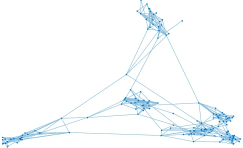
Figure 3: Topology of a simulated (sparse) network
Proof See Appendix A.3
We remark that, while a convergence rate has been established in the literature (see, e.g., Razaviyayn et al. (2014a)) for certaincentralizedalgorithms applied to special classes of DL problems, Theorem 3 represents the first rate result for adistributedalgorithm tackling the class of DL problems P.
5. Numerical Experiments
In this section, we test numerically our algorithmic framework on several classes of problems, namely: (i) Image denoising, (ii) Biclustering, (iii) Sparse PCA, and (iv) Non-negative sparse coding. We recall that D4L is the first provably convergent distributed algorithm for Problem P; comparisons are thus not simple. To give the sense of the performance of D4L, in our experiments,
(i) when available, we implemented,centralized algorithms tailored to the specific prob-lems under consideration and used the results asbenchmarks;
(ii) for undirected graphs, we extended the (distributed) Prox-PDA-IP (Zhao et al., 2016) algorithm to the simulated instances of Problem P (generalizations of this method to directed graphs seem not possible);
(iii) for both undirected and directed graphs, we implemented a suitable version of the Adapt-Then-Combine (ATC) Algorithm (Chainais and Richard, 2013). Note that ATC has no formal convergence proof, and is originally designed to handle only undirected graphs, but we managed to make a sensible extension of this method to directed graphs too, by using some of the ideas developed in this paper.
All codes are written in MATLAB 2016b, and implemented on a computer with Intel Xeon (E5-1607 v3) quad-core 3.10GHz processor and 16.0 GB of DDR4 main memory.
5.1. Image Denoising
Problem formulations: We consider denoising a 512×512 pixels image of a fishing boat (USC, 1997)−see Fig. 5(a). We simulate a cluster computer network composed of 150 nodes (computers). Denoting by F0 and F the noise-free and corrupted image, respectively, the SNR (in dB) is defined as SNR,20·log(||vec(F0)||2/
√
defined as PSNR,20·log(maxi(vec(F0))i/
√
MSE), where MSE is the Mean-Squared-Error betweenF0 and F. The fishing boat image is corrupted by additive white Gaussian noise, so that SNR = 15 dB and PSNR = 20.34 dB.
To perform the denoising task, we consider the elastic net sparse DL formulation (3). We extract 255,150 square sliding s×spixel patches (s= 8) and aggregate the vectorized extracted patches in a single data matrix Sof size 64×255,150. The size of the dictionary is s2×s2 = 64×64; the data matrix is equally distributed across the 150 nodes, resulting in sparse representation matrices Xi of size 64×1701 (K = 64 and ni = 1701). The total number of optimization variables is then 16,333,696. The free parameters λ, µ and α in (3) are set toλ= 1/s,µ=λand α= 1, respectively.
Algorithms and tuning: We tested: i) two instances of the D4L Algorithm, corresponding to two alternative choices of the surrogate functions; ii) the Prox-PDA-IP algorithm (Zhao et al., 2016), adapted to problem (3) (only on undirected networks); iii) the ATC algorithm (Chainais and Richard, 2013); and iv) thecentralized K-SVD algorithm (Elad and Aharon, 2006) (KSVD-Box v13 package), used as a benchmark. More specifically, the two instances of the D4L Algorithm are:
• Plain D4L: ˜hi is chosen as in (16) (the original function) and ˜fi as in (15);
• Linearized D4L: ˜hi is given by (17) (first-order approximation) and ˜fi is given by
(15).
The rest of the parameters in both instances of D4L is set as: γν =γν−1(1−γν−1), with
γ0 = 0.5 and= 10−2;τD,iν = 10; and τX,iν = max(L∇Xi(U ν
(i)),1) [cf. (24)].
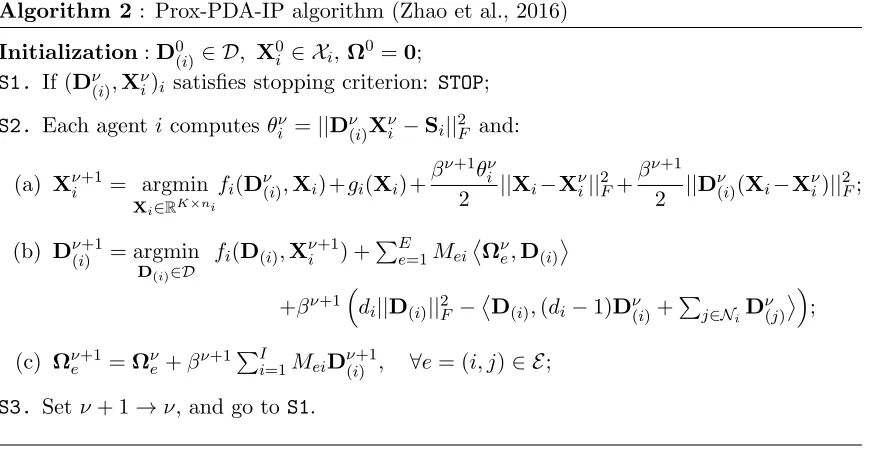
Our adaptation of the Prox-PDA-IP algorithm to Problem (3) is summarized in Al-gorithm 2. The difference with the original version in (Zhao et al., 2016) are: i) the elastic net penalty is used in the objective function for the Xi’s variables, instead of the `1-norm and `2-norm ball constraints; and ii) the variables D(i)’s are constrained in D , {D : ||Dek||2 ≤ α, k = 1,2, . . . , K} rather than using the `2-norm regularization in the objective function. The other symbols used in Algorithm 2 are: i) the incidence matrix of G, denoted by M= (Mei)e,i∈RE×I, withE ,|E|; ii) the matrices Ωνe ∈RM×K,
e= 1, ..., E, which are the ν-th iterate of the dual matrix variables Ωe ∈RM×K, as
intro-duced in the original Prox-PDA-IP; and iii) {βν}ν∈N+ is the increasing penalty parameter,
set to βν = 0.002ν.
All the algorithms are initialized to the same value: D0
(i)’s coincide with randomly (uniformly) chosen columns ofS(i)’s whereas all X0i’s are set to zero.
While the subproblems solved at each iteration ν in Linearized D4L admit a closed-form−see (23) and (22)−in both Plain D4L and ATC, the update of the dictionary has the closed form expression (22), but the update of the private variables calls for the solution of a LASSO problem (cf. Sec. 3.1). For both Plain D4L and ATC, the LASSO subproblems at iteration ν are solved using the (sub)gradient algorithm, with the following tuning. A diminishing step-size is used, set toγr=γr−1(1−γr−1), where γ0 = 0.9,= 10−3, and r
Algorithm 2 : Prox-PDA-IP algorithm (Zhao et al., 2016)
Initialization:D0
(i)∈ D, X0i ∈ Xi,Ω0 =0;
S1. If (Dν(i),Xνi)i satisfies stopping criterion: STOP;
S2. Each agent icomputes θiν =||Dν(i)Xνi −Si||2F and: (a) Xνi+1 = argmin
Xi∈RK×ni
fi(Dν(i),Xi) +gi(Xi) +
βν+1θiν
2 ||Xi−X ν i||2F+
βν+1
2 ||D ν
(i)(Xi−Xνi)||2F; (b) Dν(i+1) = argmin
D(i)∈D
fi(D(i),Xνi+1) +
PE
e=1Mei
Ωνe,D(i)
+βν+1di||D(i)||2F −
D(i),(di−1)Dν(i)+Pj∈NiD ν
(j)
;
(c) Ωνe+1=Ωνe+βν+1PI
i=1MeiDν(i+1) , ∀e= (i, j)∈ E;
S3. Setν+ 1→ν, and go to S1.
the subgradient algorithm in the inner loop whenJir≤10−6, with
Jir ,
Xν,ri − s 1 +sT1s
Xν,ri −∇Xifi(Uν(i),X
ν,r i ) +τ
ν X,i(X
ν,r
i −X
ν i)
∞,∞
,
where Xν,ri denotes the value of Xi at the r-th inner iteration and outer iteration ν; and
Tθ(x) , max(|x| −θ,0)·sign(x) is the soft-thresholding operator, applied to the matrix argument componentwise. In all our simulations, we observed that the above accuracy was reached within 30 (inner) iterations of the subgradient algorithm.
In the Prox-PDA-IP scheme, StepS2(cf. Algorithm 2) calls for the solution of two sub-problems, including a LASSO problem. As for Plain D4L and ATC, we used the (projected) (sub)-gradient algorithm (with the same diminishing step-size rule) to solve the subprob-lems; we terminated the inner loop when the length between two consecutive iterates of the (projected) (sub)-gradient algorithm goes for the first time below 10−6.
We simulated both undirected and directed static graphs. In the former case, there is no need of theφ-variables and, in the second equation of (12) [and (13)], the terms (φνjaνij)/φνi+1
reduce to aij. The weights aij are chosen according to the Metropolis-Hasting rule (Xiao et al., 2007); the resulting matrixAν = [aij]ij is thus time-invariant and doubly stochastic. When the graph is directed, we use the update of the φνi’s as in (12), with the weights aνij
chosen according to the push-sum protocol (Kempe et al., 2003) (cf. Sec. 3.1.3).
Convergence speed and quality of the reconstruction: In the first set of simulations, we considered an undirected graph composed of 150 nodes, clustered in 6 groups of 25 (see Fig. 3). Starting from this topology, we kept adding random edges till a connected graph was obtained. Specifically, an arc is added between two nodes in the same cluster (resp. different clusters) with probabilityp1 = 0.2 (resp. p2 = 2×10⁻³).
0 500 1000 1.1
1.2 1.3 1.4 1.5 1.6 10
5
0 500 1000 10-2
10-1 100
0 500 1000 10-1
100
Figure 4: Denoising problem – D4L, Prox-PDA-IP and ATC algorithms: objective value [subplot on the left], consensus disagreement [subplot in the center], and distance from stationarity ∆ν [cf. (26)] [subplot on the right] vs. number of message exchanges.
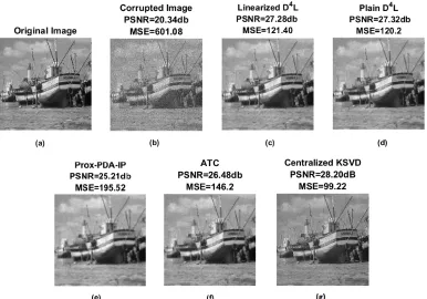
(28) [subplot on the right] versus thenumber of message exchanges, achieved by Plain D4L, Linearized D4L, Prox-PDA-IP, and ATC. Note that the number of messages exchanged in the ATC algorithm at iterationν coincides with ν whereas for Prox-PDA-IP and the D4L schemes is 2ν (recall that the latter schemes employ two steps of communications per itera-tion). The figures clearly show that both versions of D4L are much faster than Prox-PDA-IP and ATC (or, equivalently, they require fewer information exchanges). Moreover, ATC does not seem to reach a consensus on the local copies of the dictionary, while Prox-PDA-IP and D4L schemes reach an agreement quite soon. In Fig. 5, we plot the reconstructed images along with their PSNR and MSE, obtained by the algorithms, when terminated after 1000 message exchanges. The figures clearly show superior performance of D4L over its com-petitors. Also, the values of PSNR and MSE achieved by D4L are comparable with those obtained by (centralized) K-SVD (KSVD-Box v13package).
A closer look at Fig. 4 shows that a significant decay on the objective function occurs in the first 200 message exchanges. It is then interesting to check the quality of the re-constructed images, achieved by the algorithms if terminated then. In Fig. 6, we report the images and values of PSNR and MSE obtained by terminating the schemes after 200 message exchanges (we also plot the benchmark obtained by K-SVD, run till optimality). The figure shows that both versions of D4L attain high quality solutions even if terminated after few message exchanges while ATC and Prox-PDA-IP lag behind. This means that, in practice, there is no need to run D4L till very low values ofeν and ∆ν are achieved.
Figure 5: Denoising outcome. (a): original image; (b): corrupted image; (c)-(f): denois-ing achieved by D4L, Prox-PDA-IP and ATC terminated after 1000 message exchanges; and (g): denoising achieved by centralized K-SVD (KSVD-Box v13).
than Plain D4L, when terminated early; the explanation is in Table 2 which shows that the time of one iteration of the former algorithm is much shorter than that of Plain D4L.
Algorithm Average Time per Iteration (sec)
Linearized D4L 2.862
Plain D4L 11.328
Prox-PDA-IP 30.98
ATC 9.838
Table 2: D4L vs. Prox-PDA-IP and ATC: Average computation time per iteration
Impact of the graph topology and connectivity: We study now the influence of the topology and graph connectivity on the performance of the algorithms. We consider
Figure 6: Denoising outcome. (a): original image; (b): corrupted image; (c)-(f): denois-ing achieved by D4L, Prox-PDA-IP and ATC terminated after 200 message ex-changes; and (g): denoising achieved by centralized K-SVD (KSVD-Box v13).
Figure 7: Denoising outcome. (a): Linearized D4L; (b): Plain D4L; (c): Prox-PDA-IP; (d) ATC; all terminated after after 273 seconds run-time (corresponding to 200 message exchanges of the Linearized D4L).
each scenario, we generated 5 random instances (if a generated graph was not strongly connected we discarded it and generated a new one) and then ran Plain and Linearized D4L and ATC on the resulting 15 graphs. Recall that ATC was not designed to work on directed networks. We thus modified it by using our new consensus protocol (but not the gradient tracking mechanism); we term it Modified ATC.
0 500 1000 1
1.1 1.2 1.3 1.4 1.5
0 500 1000
10-8 10-6 10-4 10-2 100
0 500 1000
10-4 10-3 10-2
(a)
0 500 1000
1 1.1 1.2 1.3 1.4
1.5 10
5
0 500 1000
10-5 10-4 10-3 10-2 10-1 100
0 500 1000
10-4 10-3 10-2
(b)
0 500 1000
1 1.1 1.2 1.3 1.4
1.5 10
5
0 500 1000
10-5 10-4 10-3 10-2 10-1 100
0 500 1000
10-4 10-3 10-2
(c)
Network # I nc p1 p2
N1 500 50 0.9 0.9
N2 500 50 0.1 0.01
N3 500 50 0.05 0.01
Table 3: Network setting
and N3 [subplot (c)]. The average is taken over the aforementioned 5 digraph realizations. While also this batch of tests confirms the better behavior of D4L schemes over ATC, it is interesting to observe that there seems to be little influence of the degree of connectivity on the behavior of Linearized and Plain D4L. The only aspect for which a reasonable influence can be seen is on consensus. In fact, with respect to consensus, Linearized D4L seems to improve over Plain D4L, when connectivity decreases. This has a natural interpretation. Plain D4L solves much more accurate subproblems at each iteration and this is, in some sense useless, especially in early iterations, when information has not spread across the network. It seems clear that the less connected the graph, the more time information needs to spread. Therefore, in scenario N1, the two methods are almost equivalent and, looking at consensus error, we see that initially Linearized D4L is better than Plain D4L, but soon, as information spreads, Plain D4L becomes, even if slightly, better than Linearized D4L. The same behavior can be observed for scenario N2, but this time the initial advantage of Linearized D4L is larger and the switching point is reached much later. This is consistent with the fact that information needs more time to spread and therefore solving the accurate subproblem is not advantageous. If one passes to N3, where connectivity is very loose, there is no switching point within the first 1000 message exchanges.
5.2. Biclustering
Biclustering has been shown to be useful in several applications, including biology, infor-mation retrieval, and data mining; see, e.g., (Madeira and Oliveira, 2004).
Problem Formulation: We consider a Biclustering problem in the form (6), applied to genetic information. We solved the problem simulating a networked computer cluster composed of 500 nodes (see Table 3). The genetic data is borrowed from (Lee et al., 2010) (centered and normalized): the data matrix S of size 56×12,625 (M = 56 and
N = 12,625) contains microarray gene expressions of 56 patients (rows); each patient is either identified to be normal (Normal) or belonging to one of the following three types of lung cancer: pulmonary carcinoid tumors (Carcinoid), colon metastases (Colon), and small cell carcinoma (SmallCell). We considered theunsupervised instance of the problem, meaning that none of the a-priori information about the type of patients’ cancer is used to perform biclustering. Following the numerical experiments of (Lee et al., 2010), we seek rank-3 sparse matrices Xi, and the data matrix S is equally distributed across the 500 nodes, resulting thus inK = 3 andni = 26. The total number of variables is then 39,168. The other parameters are set as follows: α= 1, λX =µX = 0.1, andλD =µD = 0.1.
extra structure of the original function fi, plus, in case of ˜fi, there is no certain benefit in using the linear approximation (15) as it does not lead to any closed form solution of the subproblem (8). Note that the Prox-PDA-IP scheme is not applicable here since the network is directed.
The other parameters of the algorithm are set to: γν =γν−1(1−γν−1), with γ0 = 0.2 and = 10−2; andτD,iν = 100 and τX,iν = max(L∇Xi(U
ν
(i)),100). We term such an instance of D4L Plain D4L. We compared Plain D4L with the following algorithms: i) (a modi-fied version of) the distributed ATC algorithm (Chainais and Richard, 2013), where the optimization of D is adjusted to solve (6) (the elastic-net penalty is added), and the con-sensus mechanism is modified with our new concon-sensus protocol to handle directed network topologies; we termed this instanceModified ATC; and ii) the centralized SSVD algorithm proposed in Lee et al. (2010) (implemented using the MATLAB code provided by the au-thors), to benchmark the results obtained by the distributed algorithms. All the distributed algorithm are initialized setting eachX0i =0, and eachD0(i)equal to some randomly chosen columns ofSi.
In D4L, the subproblems (8) and (11) at iteration ν do not have a closed form solution; they are solved using the projected (sub)gradient algorithm, with diminishing step-size
γr =γr−1(1−γr−1), where γ0 = 0.9, = 10−3, and r denotes the inner iteration index. A warm start is used for the projected subgradient algorithm; the initial points are set to
Dν(i) and Xνi in problems (8) and (11), respectively, where ν is the iteration index of the outer loop. We terminate the projected subgradient algorithm solving (8) and (11) when
JD,ir ,kDbν,r (i) −D
ν,r
(i)k∞,∞≤10
−6 andJr
X,i,kXbν,ri −Xiν,rk∞,∞,≤10−6, respectively, where b
Dν,r(i) ,argmin
D(i)∈D
D
∇Dfi(Dν,r(i),Xνi) +IΘν(i)− ∇Dfi(Dν(i),Xνi) +τD,iν D ν,r
(i) −D
ν
(i)
,D(i)−Dν,r(i)E
+ 100 2
D(i)−D
ν,r
(i) 2
+G D(i)
,
b
Xν,ri , argmin
Xi∈RK×ni
D
∇Xifi(U ν
(i),X
ν,r i ) +τ
ν X,i(X
ν,r
i −X
ν
i),Xi−Xν,ri
E
+ 100
2 kXi−X ν,r i k
2
+gi(Xi),
with Dν,r(i) and Xν,ri denoting the value of D(i) and Xi at the ν-th outer and r-th inner iteration, respectively. In all our simulations, the above accuracy was reached within 50 (inner) iterations of the projected subgradient algorithm.
Convergence speed and quality of the reconstruction: We simulated 3directed static
0 500 1000 4500
5000 5500 6000 6500
0 500 1000
10-8 10-6 10-4 10-2 100
0 500 1000
10-4 10-3 10-2 10-1 100
(a)
0 500 1000 4500
5000 5500 6000 6500
0 500 1000 10-3
10-2 10-1 100
0 500 1000 10-4
10-3 10-2 10-1 100
(b)
0 500 1000 4500
5000 5500 6000 6500
0 500 1000 10-3
10-2 10-1 100
0 500 1000 10-4
10-3 10-2 10-1 100
(c)
In order to assess the quality of the solutions achieved by the three algorithms, we employ the following procedure. Given the limit point (up to the fixed accuracy) D∞ of the algorithm under consideration, patients’ information is in form of (unlabeled clusters of) data points {D∞m,:}56
m=1, where D∞m,: denotes the m-th row of D∞ and represents an individual patient. In order to compareD∞ with the labeled ground truth, we need to tag labels to the clustered points of D∞. To do so, we run the K-means clustering algorithm on {D∞m,:}56
m=1. Specifically, we first run K-means 100 times and, in each run, we perform a preliminary clustering using 10% of the points (randomly chosen). Then, among the 100 obtained clustering configurations, we picked the one with the smallest “within-cluster sum of point-to-centroid distances”.1 Finally, we assign to each cluster the label associated with the most populated type of cancer in the cluster. Denoting the ground truth classes by {Ci}4i=1 (recall that there are 4 classes/types of cancer), where each Ci consists of the group of patients with the same type of cancer, and by {Cei}4i=1 the clustering obtained by the procedure described above applied to the outcomeD∞of the simulated algorithms, we measure the quality of the clustering by theJaccard index, defined as
J =
S
i
Ci∩Cei
P
i
Ci∪Cei
.
Clearly 0≤J ≤1, and the higher the index value, the better the quality of the clustering. In Table 4, we report the average and Maximum Absolute Deviation (MAD) of the Jaccard indices from their average, computed over the aforementioned 5 realizations of the three graph topologies, as in Table 3 (see also Fig. 9). The values in the table clearly show that Plain D4L achieves better results than those produced by Modified ATC or centralized methods. Moreover, the value of the Jaccard index from Plain D4L does not depend on the specific network topology. which is not the case for Modified ATC.
Network # Plain D4L Modified ATC Lee et al. (2010)
N1 0.8983/0 0.7778/0 –
N2 0.8983/0 0.7045/0.3218 –
N3 0.8983/0 0.7892/0.0172 –
Centralized – – 0.7231/–
Table 4: Biclustering problem−Average/MAD of Jaccard indices over 5 realizations of di-graphs.
5.3. Non-negative Sparse Coding (NNSC) and Sparse PCA (SPCA)
Problem Formulation: We consider the Non-negative Sparse Coding (NSC) formula-tion (7) (Hoyer, 2004) and the Sparse PCA problem (6) (Mairal et al., 2010). For both formulations, we run experiments using the following two datasets:
• MIT-CBCL face database #1 (Sung, 1996): a pool of N = 2,429 vectorized face images of size 19×19 pixels each (i.e. M = 361);
1. Given a clustering partition {Ci}4i=1, the “within-cluster sum of point-to-centroid distances” mea-sures the quality of the k-means clustering, and is defined as P4
i=1
P j∈Ci||D
∞
j,: −D ∞
Ci||2, where
DCi, 1 |Ci|
P j∈CiD
∞
• The VOC 2006 database (Everingham et al., 2010): a pool of N = 10,000 vectorized natural image patches of size 16×16 pixels each (i.e. M = 256).
Consistently with (Mairal et al., 2010), the free parameters are set as:
• NNSC (7): K= 49, λ=µ= 1/√M, and α= 1; • Sparse PCA (6): K = 49, λX =µX = 1/
√
M,λD =µD = 1/
√
M, and α= 1.
The total number of variables for the above optimization problems are 136,710 for the MIT-CBCL dataset, and 502,544 for the VOC 2006 dataset.
We simulated the communication network as static directed graphs of size I, clustered inncgroups, where each node has an outgoing arc to another node in the same cluster with probabilityp1, whilep2 is the probability of an outgoing arc to a node in a different cluster. We run our tests over 6 different network scenarios, with various sizeI and probability pair (p1, p2), as given in Table 5. Note that if N/I is not an integer, we pad zero columns to the data matrix S so that all the agents own equal-size partitionsSi’s, thusni =dN/Iein both problems (6) and (7).
Network # I nc p1 p2
N4 10 2 0.9 0.3
N5 10 2 0.2 0.1
N6 50 5 0.9 0.3
N7 50 5 0.2 0.1
N8 250 10 0.9 0.3
N9 250 10 0.2 0.1
Table 5: Network setting for the NNSC and Sparse PCA problems.
5.3.1. Non-negative Sparse Coding
Algorithms and tuning: We test the Plain D4L, with ˜fi and ˜hi chosen according to (15) and (16), respectively. The other parameters of the algorithm are set to: γν = γν−1(1−
γν−1), with γ0 = 0.2 and = 10−2; and τD,iν = 10 and τX,iν = max(L∇Xi(U ν
(i)),10). We compare the proposed scheme with a modified version of ATC, equipped with our new consensus protocol, implementable on directed networks. All the distributed algorithm are initialized settingX0i =0andD0(i)equal to some randomly chosen columns ofSi. Both Plain D4L and Modified ATC call for solving a LASSO problem in updating the private variables (cf. Sec. 3.1); the update of the dictionary has instead a closed form expression, see (22). For both Plain D4L and Modified ATC, the LASSO subproblems at iterationν are solved using the projected (sub)gradient algorithm with diminishing step-size γr = γr−1(1−γr−1), where γ0 = 0.9, = 10−3, and r denoting the inner iteration index. We terminate the projected subgradient algorithm in the inner loop when JX,ir ,kXbν,ri −Xν,ri k∞,∞ ≤10−4, where
b
Xν,ri ,argmin
Xi∈Xi D
∇Xifi(U ν
(i),X
ν,r i ) +τ
ν X,i(X
ν,r
i −X
ν
i),Xi−Xν,ri
E +1
2kXi−X ν,r i k
2
and Xν,ri denotes the value of Xi at the ν-th outer and r-th inner iteration. In all our simulations, the above accuracy was reached within 30 (inner) iterations of the projected subgradient algorithm.
Convergence speed and quality of the reconstruction: We run the Plain D4L and Modified ATC algorithms over different network settings, as listed in Table 5, and we terminated them after 1500 message exchanges. We replicated the tests for 5 independent realizations and we reported the average of the final values of the objective function, the consensus disagreement, and the distance from stationarity in Table 6 and Table 7, for the MIT-CBCL and VOC 2006 datasets, respectively. In Fig. 10 and Fig. 11 (for MIT-CBCL and VOC 2006 datasets, respectively), we plot theaveragevalue (over the aforementioned 5 graph realizations) of the objective function [subplot on the left], the consensus disagreement
eν [subplot in the center], and the distance from stationarity ∆ν [subplot on the right], versus number of message exchanges, for the two extreme network scenarios N4 [subplot (a)] and N9 [subplot (b)]. These results show that the proposed Plain D4L significantly outperforms the Modified ATC algorithm. They also show a remarkable stability of Plain D4L with respect to the simulated network graphs, which is not observed for the Modified ATC, whose performance deteriorates significantly going from N4 to N9.
Network # objective value consensus disagreement distance from stationarity
N4 169.8/171.9 9.17e-7/2.9e-4 4.7e-4/8.8e-2
N5 169.9/172.2 4.5e-6/6.7e-4 5.3e-4/9.8e-2
N6 169.8/177.2 2.4e-7/1.9e-4 5.1e-4/6.3e-2
N7 169.9/177.3 1.1e-6/6.3e-4 5.5e-4/6.1e-2
N8 169.8/191.0 2.1e-7/1.2e-4 5.1e-4/2.2e-2
N9 169.8/190.9 5.8e-7/3.1e-4 6.6e-4/1.1e-2
Table 6: NNSC problem (MIT-CBCL dataset)–Plain D4L/Modified ATC algorithms: ob-jective value, consensus disagreement, and distance from stationarity obtained after 1500 message exchanges.
Network # objective value consensus disagreement distance from stationarity
N4 845.2/848.8 2.9e-6/1.3e-4 1.1e-3/4.1e-3
N5 845.9/850.1 1.5e-5/5.3e-4 1.5e-3/6.1e-3
N6 844.8/879.5 5.7e-7/2.2e-4 1.3e-3/4.4e-2
N7 844.5/879.3 1.9e-6/1.2e-3 1.3e-3/3.9e-2
N8 844.8/941.2 5.6e-7/1.5e-4 1.6e-3/4.8e-2
N9 845.0/941.8 1.5e-6/3.6e-4 1.1e-3/5.1e-2
0 500 1000 1500 160
180 200 220 240 260
0 500 1000 1500
10-8 10-6 10-4 10-2 100
0 500 1000 1500
10-4 10-3 10-2 10-1 100
(a)
0 500 1000 1500
160 180 200 220 240 260
0 500 1000 1500
10-8 10-6 10-4 10-2 100
0 500 1000 1500
10-4 10-3 10-2 10-1 100
(b)
Figure 10: NNSC problem (MIT-CBCL dataset)–Plain D4L and Modified ATC algorithms: objective value [subplots on the left], consensus disagreement [subplots in the center], and distance from stationarity ∆ν [cf. (26)] [subplots on the right] vs. number of message exchanges. Comparison over the network settings N4 [subplots (a)] and N9 [subplots (b)] (cf. Table 5).
5.3.2. Sparse Principal Component Analysis (SPCA)
Algorithms and tuning: We test the same D4L version as used in the Biclustering experiments (cf. Subsec. 5.2), i.e., ˜fi and ˜hi are chosen according to (14) and (16), re-spectively; we set γν =γν−1(1−γν−1), with γ0 = 0.2 and = 10−2; and τD,iν = 10 and
τX,iν = max(L∇Xi(U ν
(i)),10). We term it Plain D
0 500 1000 1500 800
900 1000 1100 1200 1300 1400
0 500 1000 1500 10-6
10-5 10-4 10-3 10-2 10-1
0 500 1000 1500 10-3
10-2 10-1 100
(a)
0 500 1000 1500 800
900 1000 1100 1200 1300 1400
0 500 1000 1500 10-6
10-5 10-4 10-3 10-2 10-1
0 500 1000 1500 10-3
10-2 10-1 100
(b)
Figure 11: NNSC problem (VOC 2006 dataset)–Plain D4L and Modified ATC algorithms: objective value [subplots on the left], consensus disagreement [subplots in the center], and distance from stationarity ∆ν [cf. (26)] [subplots on the right] vs. number of message exchanges. Comparison over the network settings N4 [subplots (a)] and N9 [subplots (b)] (cf. Table 5).
solving subproblem (8)) andJX,ir ≤10−4 (in solving subproblem (11)), whereJD,ir and JX,ir
are defined as those in Subsec. 5.2. In all our simulations, the above accuracy was reached within 30 (inner) iterations of the projected subgradient algorithm.

![Figure 4: Denoising problem – D4L, Prox-PDA-IP and ATC algorithms: objective value[subplot on the left], consensus disagreement [subplot in the center], and distancefrom stationarity ∆ν [cf](https://thumb-us.123doks.com/thumbv2/123dok_us/9775255.1962771/20.612.120.493.76.236/figure-denoising-algorithms-objective-consensus-disagreement-distancefrom-stationarity.webp)

![Figure 8: Denoising problem–D4L and Modified ATC algorithms: objective value [subplotson the left], consensus disagreement [subplots in the center], and distance fromstationarity ∆ν [cf.(26)] [subplots on the right] vs.number of message ex-changes](https://thumb-us.123doks.com/thumbv2/123dok_us/9775255.1962771/23.612.104.510.77.649/denoising-modied-algorithms-objective-subplotson-consensus-disagreement-fromstationarity.webp)

