AGRONOMY AND SOILS
Effect of Sample Size on Cotton Plant Mapping Analysis and Results
Glen L. Ritchie*, Jared R. Whitaker, and Guy D. Collins
G.L. Ritchie*, Department of Plant and Soil Sciences, Texas Tech University / Texas AgriLife Research, 15th and Detroit,
Lubbock, TX 79409; J.R. Whitaker, Department of Crop and Soil Sciences, University of Georgia, P.O. Box 8112, GSU. Statesboro, GA 30460; and G.D. Collins, Department of Crop and Soil Sciences, University of Georgia, P.O. Box 748, Tifton, GA 31793-0748.
*Corresponding author: [email protected]
ABSTRACT
Although cotton plant mapping has been valu-able in understanding growth and development, variation in fruit distribution among plants is a sig-nificant mapping challenge. Choosing a sample that is large enough to generate useful information, but small enough to minimize time and resources, can make plant mapping more accessible for evaluating cotton crop growth characteristics throughout the
cotton belt. The purpose of this research was to iden
-tify the effects of sample size and main-stem node grouping on sample variability. Plants were sampled in 10-m sections from six cotton cultivars at five lo-cations in Georgia in 2009 and one location in 2010. The relative errors associated with sample sizes of
one to 50 plants, as well as the statistical power as-sociated with each sample size, were computed. On average, 37 plants per cultivar among five cultivars were required to reach a statistical power of 0.90, with the required number based on the magnitude of difference between cultivars in the fraction of plants having a boll at a given fruiting site. Grouping of main-stem nodes and the use of moving weighted averages decreased the error on a node-by-node basis. The use of these methods resulted in the loss of some node-by-node information that might be of value in particular cases, but the number of plants required to generate the same statistical power and standard deviation was decreased from a mean of 37 to a mean of 19 plants. These techniques should allow the use of smaller plant samples and make plant mapping more accessible.
T
he production and retention of cotton fruit throughout the plant canopy varies with cultivarand is sensitive to management, environmental
conditions, and biological influences (Kerbyet al., 2010). Planting mapping of fruit locations by main-stem node and sympodial fruiting position within the plant canopy is an important part of cotton research. The understanding of fruiting distribution has allowed researchers to decipher data observed
in cotton yields and fiber quality more adequately.
Cotton fruiting occurs over a period of several
weeks, with flowering occurring on vertical
main-stem nodes up the plant on a 2- to 3-d interval and on adjacent fruiting positions on the same node on a 3- to
5-d interval (Bednarz and Nichols, 2005). Mapping
might take several forms, but often consists of count-ing the cotton fruit at each fruitcount-ing site: the individual node and fruiting position of each fruit on the plant.
Fruit on different parts of the plant are at different maturity stages during times of periodic stress, insect pressure, or other factors that might affect growth. Be-cause most of the plants within a cohort are at similar growth stages at a given time, fruit production and
shedding can follow identifiable patterns among plants
in a sample. End-of-season monitoring can be linked to crop history to show where and when the plants produced most of their crop, as well as what might
have negatively impacted yield (Kerbyet al., 2010). Cotton has been shown to have different fruit de-velopment and distribution patterns based on several factors, including cultivar, plant density, and plant
growth regulator (PGR) application (Bednarzet al., 2000; Dumka, 2002; Dumkaet al., 2004). Moisture
deficit has also been shown to affect boll distribution, as shown by Pettigrew (Pettigrew, 2004a, 2004b) and Ritchie et al. (2009). Differences in yield distribution and fiber quality have been observed based on cultivar and genetic technology (Baueret al., 2009; Millset al.,
2008). All of these findings have helped expand the
knowledge of cotton growth and developmental habits.
Current Plant Mapping Methods. Plant
map-ping can take the form of either in-season
measure-ments of the production and growth of fruit (Bednarz and Nichols, 2005; McClelland, 1916), or end-of-the
season measurements of boll yield components, such
as node-by-node boll fraction (the fraction of plants
and fiber content and quality (Bauer et al., 2009;
Bednarz and Nichols, 2005; Pettigrew, 2004b). Bauer et al. (2009) and Bednarz et al. (2006) both identi
-fied differences in fiber quality parameters within
different regions of the plant.
One question that has arisen regarding the use of plant mapping is the number of plants required to provide adequate statistical power to separate
differences in treatments while using labor and time
resources efficiently. Within a representative sample
composed of multiple plants, some nodes and fruit-ing positions exhibit higher or lower fractions of fruit, but it is unusual for every plant within a sample to consistently have fruit on any single fruiting site.
Furthermore, competition between plants, as well as between fruiting sites on an individual plant, can
af-fect boll distribution (Boquet and Moser, 2003; Kerby
and Buxton, 1981; Pettigrew, 1994). Plant mapping in any form is a time-consuming process, and additional measurements such as boll mass and lint percentage can limit the scope of the process to only a relatively few samples per year. Researchers have tried varying
sample sizes, including plant areas such as 0.5 to 1.0
m2 of row (Sadras et al., 1997), 1 m2 of row comprising
about seven plants (Constable, 1991), row lengths of 1 m (Pettigrew, 2004b), 2 m (Cook and Kennedy, 2000), and 3 m (Bednarz and Roberts, 2001; Bednarz and Nichols, 2005; Mills et al., 2008) to plant counts of 10 (Vories and Glover, 2006) or 20 plants (Boquet and Moser, 2003; Boquet et al., 1994). The variation in sample size
between studies shows the balance that researchers try to make between having an appropriately large sample
size and limiting the numbers of plants in a sample to
save time or allow additional plots to be measured.
Statistical Power and Plant Mapping. The use
of statistical power has been used successfully in bio-logical research to determine the associated risks of overlooking real differences between treatments due
to insufficient sample size (Thomas and Juanes, 1996). Statistical power is the probability of a significant
population difference resulting in a statistically
sig-nificant sample difference, and measures the sample size required to maintain a significant result if the null hypothesis is false. Specifically, a test of statistical
power estimates the Type II error: the risk of a real result being masked by a test that is not sensitive enough to detect treatment differences. An analysis of the statisti-cal power of different subsample row lengths should
give insight on the proper subsample size to minimize the risk of overlooking significant differences while
limiting the number of plants that must be sampled.
Data Smoothing. In addition to determining
vari-ability and statistical probvari-ability on a node-by-node basis, it might be possible to decrease variability and therefore improve statistical power through the use
of node grouping or smoothing techniques (Savitzky
and Golay, 1964). Grouping nodes together decreases the effects of node-to-node variability in the sample by taking into account adjacent nodes. However, the grouping of nodes limits information to broad areas of the plant. This method is likely appropriate in ex-periments resulting in small treatment effects on boll distribution where differences between individual nodes are subtle, but overall differences within a
region of the plant may be significant.
Smoothing can also be used as a method to de-crease variability, and is also widely used as a method of statistical “noise” removal in many facets of
sci-ence, including spectrometry (Demetriades-Shahet al., 1990; Elvidge and Chen, 1995), speech recognition
(Kulkarni and Colburn, 1998), and time series analysis (Chen et al., 2004). A smoothing function uses values
from adjacent data points to decrease point-to-point variation over a series. The purpose of smoothing is to remove small scale variations and noise from a spectrum or time series, while preserving most of the useful features. In the case of boll distribution mea-surements, decreasing node-to-node variability with a
smoothing function should significantly decrease the
error, and therefore, the number of plants that would be needed for a strong analysis.
Our objectives in this study were to measure the relative error associated with different subsample populations within a plot to give more clarity to the plant mapping process and test methods of de-creasing the associated error without inde-creasing the number of plants being sampled. With this additional
information, the use of plant mapping techniques can be expanded without increasing the time required.
MATERIALS AND METHODS
Nonirrigated county variety trial locations in Burke, Colquitt, Coffee, and Jefferson counties in
Georgia, and an irrigated trial in Coffee County were used as locations for data collection in 2009. The trials were conducted under the direction of county extension agents and extension specialists throughout South Georgia and East Georgia. At each location, 10 m of linear row were selected in each of six cultivars:
(DP0935), Stoneville 5458 B2RF (ST5458), Fiber
-Max 1740 B2RF (FM1740), and Phytogen 375 WRF (PHY375). These cultivars were chosen for their wide
-spread use in Georgia and their unique fruiting habits.
Data Collection. Plant heights and spaces between
plants were measured for each individual plant within the 10 m of row, and all plants were mapped that were at least 45 cm tall and had at least one viable fruit. Plant mapping consisted of counting all harvestable fruit by fruiting site on both vegetative and reproductive branches on each individual plant. Bolls produced by vegetative branches were summed across the entire plant and the main-stem node and sympodial fruiting position were recorded for each boll produced on a fruiting branch. Total main-stem nodes for each plant
were also measured. Plant density ranged from five to eight plants per square meter and varied by location and
cultivar. Data were collected between 2 and 10 d prior to harvest, and at least 1 wk after defoliation. Harvest data included plot length and seed cotton weight for the entire plot, and 100 kg subsamples were ginned at
the University of Georgia Microgin.
Analysis. After mapping was completed, the
ef-fects of sample size were analyzed by grouping every
possible range of 1 m, 1.5 m, 2 m, and 3 m of plants in a linear row as individual samples and measuring the relative error from the means of each grouping
size for each node and fruiting position.
The effects of using basic selection procedures to determine fruit distribution on a plant-by-plant basis were also tested with samples of 5, 10, 15, and 20 plants. Plants with apical meristem damage below node 15 that caused loss of apical dominance, plants that were more than one standard deviation shorter than the cultivar mean at each location, and individual plants with a cumulative gap between adjacent plants of greater than 40 cm were eliminated from the analy-sis. This method simulated basic decision making in a trial situation to eliminate nonrepresentative plants and potentially give a more precise estimate without an increase in the amount of sampling. Because the purpose of the study was to determine the relative
uncertainty of different sample sizes, the standard deviation generated with each sample size and method
was used as a basis for measuring relative error. The error ratio was calculated by measuring the standard deviation at all existing plant boll populations
for each sample size (sn plants), regressing the error to
the error for one-plant samples (s1 plant), forcing the
intercept to 0, and measuring the slope, or ratio, as sn
plants / s1 plant. This allowed comparison over the entire
range of boll fractions from the samples, even though the standard deviation varied based on boll fraction between nodes and cultivars. The same calculation was performed with smoothed data at the same plant
sample sizes, and the error ratio was calculated based
on the unsmoothed s1 plant to show the relative decrease
in error compared to unsmoothed data.
Power analysis was also performed in SAS 9.2
(SAS Institute, Inc., Cary, NC) using PROC POWER
to measure the number of samples necessary to have
a reasonable certainty (statistical power of 0.9) of differences by node between cultivars in the five
environments. The standard deviations of the full 10-m plot lengths were used as the standard deviation
for the power analysis.
RESULTS AND DISCUSSION
Plant Number and Relative Error. Standard
deviation was closely related to the percentage of
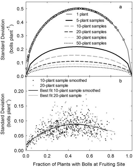
plants with bolls at a specific node and position (Fig. 1a) over a wide range of sample sizes. Counting bolls
on a plant-by-plant basis results in a binary dataset: each plant either has or does not have a boll at a
specific node and position.
As shown in Fig. 1a, the relationship between measured standard deviations and boll fraction fol-lowed a very predictable model. The standard
devia-tion lines by sample size in Fig. 1a were derived from a
10,000-sample binary dataset, but none of the standard deviation measurements by location varied from the single-plant standard deviation line, even though bolls were not necessarily randomly distributed among the plants in the samples. Grouping plants together resulted in variations in the standard deviation by
boll fraction, due to the increase in the sample size compared to the population size, the decrease in the
number of samples, and the effects of nonrandom
distribution of bolls within the population (Fig. 1b).
The accumulation of additional plants within a sam-ple approximates a continuous dataset as samsam-ple popula-tion increases. At high and low proporpopula-tions of plants with fruit at a given node and position, the standard deviations were low even at low sample populations, because there were fewer samples that varied from the mean. However, as the ratio of plants with a boll approached 0.5, the standard deviation within a group of individual plants
The decrease in the s1 plant / sn plants ratio with the
addition of plants was nonlinear, becoming less
pronounced as plant number increased (Fig. 2). Measuring five plants instead of one decreased the
standard deviation by 56%, and the use of 10 plants decreased the standard deviation by 70%. The addi-tion of plants into a sample greater than 10 plants had increasingly smaller effects on standard deviation: 20 plants decreased the standard deviation by 79%, 50 plants decreased it by 87%, and 100 plants by 91%.
Power analysis for cultivar separation for first
position fruit at each node showed the number of
samples required for a statistical power of 0.9 (10% or
less Type II error) to range from 9 to 141 with a mean of 41-plant samples and a median of 32-plant samples
(Table 1). Nodes and locations with smaller ranges of differences between cultivars required higher numbers
of samples to reach a statistical power of 0.9, with particularly high numbers occurring when all pairwise differences in the boll fraction between cultivars at a
specific node were less than 0.07.
The standard deviation versus sample size com -parisons for both plot-length measurements and plant-number measurements resulted in nearly identical relationships, even though stunted plants, damaged plants, and plants with large gaps around them were removed from the plant-number measurements and
not from plot-length measurements (Fig. 3). However,
the seeming lack of effect by removing nonstandard plants might be misleading. Standard deviation is measured from the population at large, and changes in fruiting at a given fruiting site for a single plant affect both the overall fruit proportion and the associated
standard deviation. Measurement of standard devia -tion does not directly take into account the effects on fruit proportion, so nonstandard plants have no
different effect on boll fraction at a specific fruiting
site than any other plant. However, mapping unusual plants can increase or decrease the measured boll frac-tion outside of the natural range among typical plants.
Grouping of Adjacent Nodes and Smoothing.
The grouping of adjacent nodes was shown to decrease measurement error, as measured by standard deviation,
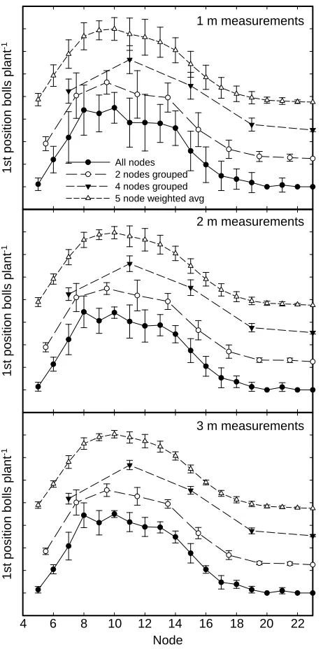
and decrease the number of plants required to reach a given standard deviation (Fig. 4). Combining groups
of two nodes resulted in a small decrease in error for all measurement lengths, and combining groups of four nodes decreased measurement error substantially at all measurement lengths. However, some of the ability to assess growth habits was lost by combining additional
nodes into zones. For the four-node groupings, mea
-surements of unique values were decreased from 19 to 5. Figure 1. Relationship between fraction of plants with bolls
and standard deviation (a) for five sample sizes with a
random distribution of plants with and without bolls and (b) with 10-plant samples with data smoothing and
20-plant samples without data smoothing.
Number of plants in sample
0 10 20 30 40 50
E
rr
o
r
ra
ti
o
(sn
plant
s
:s1
plant
uns
m
oot
hed
)
0.0 0.2 0.4 0.6 0.8 1.0
Smoothing applied No smoothing
Figure 2. Relative standard deviation (sn plants / s1 plant unsmoothed)
based on the number of plants in a plant mapping sample
compared to that of a single plant. The black line represents
measurements taken from individual nodes with no
smoothing. The gray line represents a five-node weighted average moving window smoothing function. Error bars
represent the standard error of the individual sn plants / s1 plant unsmoothed ratios for each number of plants. The horizontal
lines indicate the relative error at 30 and 50 plants for the
The use of a moving average was tested and found to decrease standard deviation while
main-taining some of the node-to-node variability (Fig. 4).
The characteristics of a moving average with both
a numerical mean (equivalent to grouping adjacent
nodes with a moving window for each node) and a weighted mean were found to have similar effects on the data, but with slight differences. The numerical means resulted in slightly lower standard deviations on a node-by-node basis, but the deviations from the mean of the unsmoothed data were larger than with
the weighted mean method (data not shown), sug -gesting an increased loss of resolution due to the nu-merical mean. Because the differences between the numerical mean and the weighted mean were small, the weighted mean was used for additional analysis
to decrease variability while minimizing variations
from the unsmoothed data. Using a weighted mean
decreased the number of plants required per sample to give a significant result between cultivars (Table 1), generally decreasing the sample size require
-ments in half.
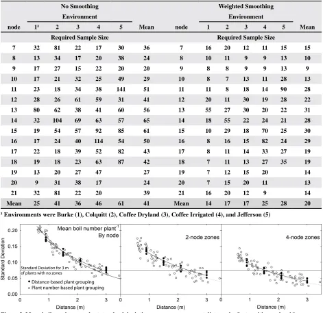
Figure 3. Mean boll number per plant standard deviation versus measurement distance by first position node with no zones, two-node zones, and four-node zones. A reference line is added for comparison of the relative error of each zone method compared to a 3-m sample with no zones.
Table 1. Power analysis for cultivar mean separation at all locations. Sample size represents the plant sample size required to obtain a statistical power of 0.9 for first position boll differences between cultivars
No Smoothing Weighted Smoothing
Environment Environment
node 1z 2 3 4 5 Mean node 1 2 3 4 5 Mean
Required Sample Size Required Sample Size
7 32 81 22 17 30 36 7 16 20 12 11 15 15
8 13 34 17 20 38 24 8 10 11 9 9 13 10
9 17 27 15 22 20 20 9 8 8 9 9 13 9
10 17 21 32 25 49 29 10 8 7 13 11 28 13
11 23 18 34 38 141 51 11 11 8 18 14 90 28
12 28 26 61 59 31 41 12 20 11 30 19 28 22
13 80 62 38 41 60 56 13 55 27 30 20 22 31
14 32 104 69 63 57 65 14 18 55 22 24 21 28
15 19 54 57 92 85 61 15 10 29 18 70 25 30
16 17 24 40 114 54 50 16 8 16 15 82 24 29
17 22 18 39 52 82 43 17 8 11 14 33 27 19
18 19 18 23 63 87 42 18 7 11 13 27 35 19
19 13 20 27 47 27 19 7 12 15 20 14
20 9 31 38 17 24 20 7 15 20 11 13
21 32 81 22 20 39 21 16 20 12 9 14
Mean 25 41 36 46 61 41 Mean 14 17 17 25 28 20
The use of the five-node smoothing procedure resulted in lower numbers of plants required to
reach low s1 plant / sn plants ratios (Fig. 2). The s1 plant
/ sn plants ratio of a group of 10-plant samples with
smoothed data was almost identical to the error ratio obtained with a group of 30-plant samples and no smoothing. The s1 plant / sn plants ratio with
50-plant samples and no smoothing could be
duplicated with 17-plant samples and smooth-ing. Similarly, the use of a 10-plant sample with smoothing resulted in an almost identical standard deviation by boll fraction as the use of a 20-plant
sample with no smoothing (Fig. 1b).
The effects of smoothing on different plant
sample sizes are shown in Fig. 5. For a single plant,
the acute differences between present and absent bolls were muted by the smoothing, but the distri-bution did not resemble the overall boll distridistri-bution.
However, with five plants in a sample, the smoothed
data already resembled the data with 50 plants in a
sample. Most of the plants at the beginning of the
measurement row did not have bolls at node 12, whereas most of the plants near the end of the row did have bolls at node 12. Therefore, lower populations
had significant deviations from the 50-plant sample,
whether smoothing was applied or not. However, the differences were spread out over a broader node region when the data were smoothed, so the differ-ences were less apparent.
Figure 4. Means and standard deviations at individual nodes, with two- and four-node groupings, and with a five-node
weighted average for all nodes at 1 m, 2 m, and 3 m spacing
using data from the DP0935 plot at location 2. For node
groupings, values are calculated at the midpoint of each
grouping. Ticks represent 0.2 fruit per plant, and node groupings are offset by 0.25 to allow comparisons.
Node
4 6 8 10 12 14 16 18 20 22
1st position b
olls plant
-1
1st position b
olls plant
-1
All nodes 2 nodes grouped 4 nodes grouped 5 node weighted avg
1st position b
olls plant
-1
1 m measurements
2 m measurements
3 m measurements
Fruiting node
5 10 15 20
1s
t po
si
tio
n
bo
ll
fra
ct
io
n
(b
ol
ls
p
la
nt
-1)
Fruiting node
5 10 15 20
1 plant 2 plants 5 plants 10 plants 20 plants 50 plants
1 plant 2 plants 5 plants 10 plants 20 plants
50 plants Unsmoothed Smoothed
Figure 5. Effects of smoothing on first position boll distribution in sample sizes ranging from 1 to 50 plants. Boll fraction data are offset by 0.5 to allow comparisons.
The dotted grey line represents the 50-plant sample for the
corresponding method.
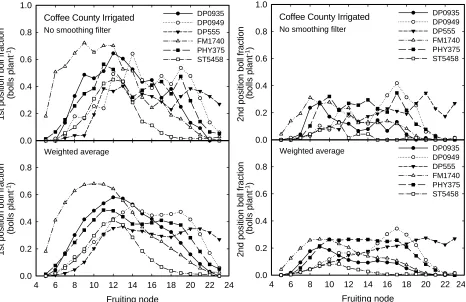
In research where heavy emphasis is placed on
boll fraction at a specific fruiting site, smoothing the
data might hide some of the effects. However, when overall distribution is of interest, smoothing results in cleaner data. As shown in Fig. 6, use of a weighted average can make overall boll fraction trends much
more distinct, both for first- and second-position fruit.
Sequential Sampling and Plant Smoothing.
One suggested method of decreasing the amount
of time measuring samples is the use of sequential sampling methods. Sequential sampling methods
have been used for more than 50 y in insect
scout-ing (Waters, 1955; Morris 1960), and are based
on the concept that when there are either high or low populations of an item of interest, fewer
samples are required to accurately estimate the population. A similar level of confidence can be
obtained from a few plants if nearly every plant has a boll present at a given fruiting site, as with a larger sample where the plants are evenly divided between having and not having a boll at a given fruiting site.
Counting bolls would certainly follow this con-ceptual model, but there are at least three factors that should be considered when using this method in plant mapping. These factors include whether more than one fruiting site is of interest in the study, the effects of adjacent fruiting sites on the site of interest, and whether smoothing will be applied.
Unless only one fruiting site is of interest in the study, each fruiting site encountered will have a dif-ferent boll complement across a sample of multiple
plants. Therefore, a simple measure of the number
of plants required for a measurement is complicated
by the differences between boll fractions at different fruiting sites. Because many of the differences in fruiting distribution between plants occur on parts of the plant where fruit retention is not high, there is a risk of choosing too few plants to ascertain differ-ences if sampling is limited by the number of plants measured due to high boll retention at another part of the plant.
The second consideration is the effect of
ad-jacent fruiting sites on boll distribution. Kerby and Buxton (1981) determined that when a fruit
is lost, adjacent fruiting sites are more likely to retain bolls. Plant-to-plant variability can result in compensation on different fruiting sites, so a focus on an individual fruiting site will sometimes over-look the effects of adjacent sites. Using smoothing methods can reduce the effects of site-to-site vari-ability, as well as take into account the effects of adjacent fruiting sites. However, smoothing also makes determination of the proper number of
plants to measure difficult, because an estimate
of the boll fraction is not tied completely to any single fruiting site.
1st position boll fraction
0.0 0.2 0.4 0.6 0.8 1.0
DP0935 DP0949 DP555 FM1740 PHY375 ST5458
Fruiting node
4 6 8 10 12 14 16 18 20 22 24
1st position boll fraction
(bo
lls
pl
an
t
-1)
(bo
lls
pl
an
t
-1)
(bo
lls
pl
an
t
-1)
(bo
lls
pl
an
t
-1)
0.0 0.2 0.4 0.6 0.8
Coffee County Irrigated
No smoothing filter
Weighted average
2nd position boll fraction
0.0 0.2 0.4 0.6 0.8 1.0
DP0935 DP0949 DP555 FM1740 PHY375 ST5458
Fruiting node
4 6 8 10 12 14 16 18 20 22 24
2nd position boll fraction
0.0 0.2 0.4 0.6 0.8
DP0935 DP0949 DP555 FM1740 PHY375 ST5458
Coffee County Irrigated
No smoothing filter
Weighted average
CONCLUSIONS
The question of how many plants to sample for
an accurate representation of boll distribution does not have a simple answer, because variance at each fruiting site is directly related to boll fraction, and each fruiting site has its own boll fraction. Further-more, the very factors that plant mapping measures, such as cultivar, irrigation, and chemical application
effects, influence growth habits and make prior de
-termination of treatment effects difficult over a range
of multiple fruiting sites. Because many of the dif-ferences due to these factors are observed in regions of the plant with low-to-medium boll fractions, it is
advisable to determine the number of plants required
based on the highest standard deviation for a sample with a given number of plants. However, the use of smoothing can decrease the number of samples
required to reach a set standard deviation, regardless
of the initial boll fraction.
In our research, increasing the number of plants in a sample decreased the standard deviation, with
sample sizes of 10 plants or more resulting in stan -dard deviations that became marginally lower with the addition of each additional plant. Grouping nodes or subjecting the data to a moving average decreased variance within a sample, in most cases decreasing
the number of plants required to reach a critical statistical power by half. Although sample sizes of
40 plants were necessary in many cases to reach a statistical power of 0.9 without moving averages, the use of multiple replicates can be used to reach this number in cases where plant growth is similar between replicates.
There is a risk with moving averages that some of the underlying individual node data might be lost, particularly in cases where outside factors might af-fect fruit production or retention for a short period of time. Some outside factors that can affect fruit retention over a short period of time include insect damage, periodic drought stress, and periods of
temperature extremes (Bednarz and Roberts, 2001; Bednarz and Nichols, 2005; Burke, 2003). Therefore,
different trends might be observed in analysis by individual node than are observed when the nodes are subjected to smoothing.
Yield distribution measurements offer the poten
-tial of significant insights into cotton development
and yield potential, which might have been
over-looked due to the time required to perform mapping and the complexity of analyzing a crop that has
multiple nodes and fruiting positions concurrently producing and shedding fruit. Smoothing might give additional insights into interactions between fruiting positions by decreasing node-by-node variation and clarifying patterns that might otherwise be overshad-owed by noise.
A suitable sample size will depend upon both
the overall boll fraction and upon variability within a sample. Additionally, variability between replicates can
affect necessary sample size. However, in cases where boll distribution is significantly different between treat -ments, a sample of 30 to 40 plants should be enough to see this difference. If boll distribution does not differ
substantially between replicates, sample sizes that re -sult in the sampling of 8 to 10 plants within a replicate
should suffice. Using smoothing functions can further decrease sample size, with the required sample size
being decreased by half in our testing.
ACKNOWLEDGMENTS
The authors would like to thank Lola Sexton, Jerry Davis, and Rebecca Hickey, who provided technical help on this project. The project received support from the Georgia Agricultural Commodity Commission for Cotton.
REFERENCES
Bauer, P.J., J.A. Foulk, G.R. Gamble, and E.J. Sadler. 2009.
A comparison of two cotton cultivars differing in
matu-rity for within-canopy fiber property variation. Crop Sci. 49:651–657.
Bednarz, C.W., and P.M. Roberts. 2001. Spatial yield distri
-bution in cotton following early-season floral bud removal. Crop Sci. 41:1800–1808.
Bednarz, C.W., and R.L. Nichols. 2005. Phenological and morphological components of cotton crop maturity. Crop Sci. 45:1497–1503.
Bednarz, C.W., D.C. Bridges, and S.M. Brown. 2000. Analy
-sis of cotton yield stability across population densities. Agron. J. 92:128–135.
Bednarz, C.W., R.L. Nichols, and S.M. Brown. 2006. Plant density modifies within-canopy cotton fiber quality. Crop Sci. 46:950–956.
Boquet, D.J., E.B. Moser, and G.A. Breitenback. 1994. Boll weight and within-plant yield distribution in field-grown cotton given different levels of nitrogen. Agron. J. 86:20–26.
Burke, J.J. 2003. Sprinkler-induced flower losses and yield reductions in cotton ( L.). Agron. J. 95:709–714.
Chen, J., P. Jönsson, M. Tamura, Z. Gu, B. Matsushita, and L. Eklundh. 2004. A simple method for reconstructing
a high-quality NDVI time-series data set based on the
Savitzky-Golay filter. Remote Sens. Environ. 91:332–344.
Constable, G. 1991. Mapping the production and survival of fruit on field-grown cotton.Agron. J. 83:374–378.
Cook, D.R., and C.W. Kennedy. 2000. Early flower bud loss and mepiquat chloride effects on cotton yield distribution. Crop Sci. 40:1678–1684.
Demetriades-Shah, T.H., M.D. Steven, and J.A. Clark. 1990. High resolution derivative spectra in remote sensing. Re
-mote Sens. Environ. 33:55–64.
Dumka, D. 2002. Efficacy of delayed fruiting in improving drought tolerance of cotton (Gossypium hirsutum. L.) in Georgia, University of Georgia.
Dumka, D., C.W. Bednarz, and B.W. Maw. 2004. Delayed
initiation of fruiting as a mechanism of improved drought
avoidance in cotton. Crop Sci. 44:528–534.
Elvidge, C.D., and Z. Chen. 1995. Comparison of broad-band and narrow-band red and near-infrared vegetation indices. Remote Sens. Environ. 54:38–48.
Kerby, T.A., and D.R. Buxton. 1981. Competition between adjacent fruiting forms in cotton. Agron. J. 73:867–871.
Kerby, T.A., F.M. Bourland, and K.D. Hake. 2010. Physi
-ological rationales in plant monitoring and mapping, p.
304–317, In J. M. Stewart, et al., eds. Physiology of Cotton.
Springer, New York.
Kulkarni, A., and H.S. Colburn. 1998. Role of spectral detail in sound-source localization. Nature 396:747–749.
McClelland, C.K. 1916. On the regularity of blooming in the cotton plant. Science 44:578–581.
Mills, C.I., C.W. Bednarz, G.L. Ritchie, and J.R. Whitaker. 2008. Yield, quality, and fruit distribution in Bollgard/
Roundup Ready and Bollgard II/Roundup Ready Flex
Cottons. Crop Sci. 100:35–41.
Morris, R.F. 1960. Sampling insect populations. Ann. Rev. of Entomol. 5:243–264.
Pettigrew, W.T. 1994. Source-to-sink manipulation effects on cotton lint yield and yield components. Agron. J. 86:731–735.
Pettigrew, W.T. 2004a. Physiological consequences of mois
-ture deficit stress in cotton. Crop Sci. 44:1265–1272.
Pettigrew, W.T. 2004b. Moisture deficit effects on cotton lint yield, yield components, and boll distribution. Agron. J. 96:377–383.
Ritchie, G.L., J.R. Whitaker, C.W. Bednarz, and J.E. Hook. 2009. Subsurface drip and overhead irrigation: A com
-parison of plant boll distribution in upland cotton. Agron. J. 101:1336–1344.
Sadras, V.O., M.P. Bange, and S.P. Milroy. 1997. Reproduc -tive allocation of cotton in response to plant and
environ-mental factors. Ann. Bot. 80:75–81.
Savitzky, A., and M.J.E. Golay. 1964. Smoothing and dif
-ferentiation of data by simplified least squares procedures. Anal. Chem. 36:1627–1639.
Thomas, L., and F. Juanes. 1996. The importance of statisti -cal power analysis: An example from Animal Behaviour.
Anim. Behav. 52:856–859.
Vories, E.D., and R.E. Glover. 2006. Comparison of growth
and yield components of conventional and ultra-narrow
row cotton. J. Cotton Sci. 10:235–243.