Max Planck Institute for Demographic Research Konrad-Zuse Str. 1, D-18057 Rostock·GERMANY www.demographic-research.org
DEMOGRAPHIC RESEARCH
VOLUME 24, ARTICLE 4, PAGES 113-144
PUBLISHED 28 JANUARY 2011
http://www.demographic-research.org/Volumes/Vol24/4/ DOI: 10.4054/DemRes.2011.24.4
Research Article
The crossover between life expectancies
at birth and at age one:
The imbalance in the life table
Vladimir Canudas-Romo
Stan Becker
c
°2011 Vladimir Canudas-Romo & Stan Becker.
2 Data 116
3 Methods 118
3.1 The crossing in life expectancies 118
3.2 The difference in life expectancies and its components 120
4 Results 122
4.1 The crossover in industrialized countries 122
4.2 The crossover in countries of the world 129
4.3 The imbalance in the life tables for the black and white populations of the USA 130
5 Discussion 132
References 136
The crossover between life expectancies at birth and at age one:
The imbalance in the life table
Vladimir Canudas-Romo1
Stan Becker2
Abstract
The single most used demographic measure to describe population health is life expectancy at birth, but life expectancies at ages other than zero are also used in the study of human longevity. Our intuition tells us that the longest life expectancy is that of a newborn. However, historically, the expectation of life at age one (e1) has
exceeded the expectation of life at birth (e0). The crossover betweene0 and e1 only
occurred in the developed world in the second half of the twentieth century. Life tables for populations that have not achieved this crossing between life expectancy at birth and at age one are referred to here as imbalanced. This crossover occurs when infant mortality is equal to the inverse of life expectancy at age one. This simple relation between mortality at age zero and mortality after age one divides the world into countries that have achieved the crossover in life expectancies and those that have not. It is a within-population comparison of mortality at infancy and after age one. However, results of these within-population comparisons can be used for comparison between populations. For countries that have already achieved this crossing in life expectancies, the sex differential in the timing of the crossing is marked: Females attain the crossing before males for every single population and in some cases by up to 18 years earlier. However, for most developing countries, life expectancy at age one is still higher than life expectancy at birth, in some cases by several years. Subpopulation comparisons for the US show that black Americans are near to transitioning out of the imbalanced life table situation while the white population has already done so.
1Department of Biostatistics, University of Copenhagen, Denmark.
Department of Population, Family and Reproductive Health, Johns Hopkins Bloomberg School of Public Health, Baltimore, USA. 615 N Wolfe Street, Room E4634, Baltimore MD 21205. Ph: (410) 955-8694, Fax: (410) 955-2303. E-mail: [email protected].
2Department of Population, Family and Reproductive Health, Johns Hopkins Bloomberg School of Public
1. Introduction
Since the 1920s and 1930s, the summary indicator most widely used to describe population health is life expectancy at birth,e0(Robine 2006; Dublin 1923; Dublin and
Lotka 1934). Period life expectancy at birth is defined as the average number of years that a newborn would live given a set of death rates observed in a calendar year (Preston, Heuveline, and Guillot 2001). Changes in mortality in the first year of life strongly affect life expectancy at birth, and it has been suggested that the time series ofe0alone is not
well suited for studying the length of life in aging populations (Kannisto 2001). This could be circumvented if both infant mortality and life expectancy at age one are used as comparative measures of the level of mortality in a population (Kintner 2004). Infant mortality levels can be compared over time, or over subpopulations defined in terms of sex, race, nationality, education, social class, etc. (Frisbie et al. 2004; Martin et al. 2005; Hummer et al. 2007). Another comparison can be made by observing the relation between the level of infant mortality in a population and its mortality at adult ages (Finch and Crimmins 2004; Galobardes, Lynch, and Smith 2004). In this study we address an alternative comparison by analyzing the crossover between life expectancy at birth and at age one, which relates the information of infant mortality to mortality at other ages.
For high-income countries, thee0calculated from period life tables is currently higher
than the life expectancy at any other age. In historical populations as well as in most developing countries, however, high rates of infant and early childhood mortality result in lower values of life expectancy at birth than at other ages. In such populations, those surviving the hazards of early childhood have a higher life expectancy than newborns and the highest life expectancy occurs not at birth but at a later age. Let an imbalance in a life table be defined as a situation where levels of life expectancy at a younger agex,ex,
are lower than at an older agey,ey, this can be expressed asex< ey whenx < y. Of
particular interest is the case of an imbalance between life expectancy at birthe0and at age
onee1, with the latter having higher values,e0< e1. Here we show how the mathematical
relations of the life table allow us to find the precise moment when this imbalance stops existing which relates life expectancies at birth and at age one, and infant mortality.
Studies of time trends in life expectancy generally focus on a fixed age, and little attention has been given to the relation to or imbalance between life expectancies at other ages. Oeppen and Vaupel (2002) concentrated on female life expectancy at birth in the specific countries holding the record value and its constant rate of increase since 1840. White (2002) fitted straight lines to the time trend ofe0in western industrialized countries
during the second half of the 20th century. Vallin and Meslé (2009) revised Oeppen and Vaupel’s findings describing the series ofe0 as multiple segments that correspond
(Riley 2005), across all countries initial increases ine0were mainly due to considerable
reductions in early life mortality. Later and ongoing gains in life expectancy are the result of mortality declines at older ages (Horiuchi 1991; Kannisto et al. 1994; Wilmoth 2000). However, life expectancy at birth alone cannot distinguish these changing stages of mortality reductions.
In the second half of the twentieth century in developed countries, life expectancy by age became a monotonic decreasing function with increasing age. However, in the past this was not the case. Figure 1 presents life expectancy by age at different times for the population of the Netherlands. In 1850 life expectancy at birth was only higher than life expectancies after age 21. Over time this changed and by 1950 the only remaining life expectancy higher thane0wase1. These substantial gaps between the life expectancy at
birth and life expectancy at age one can be found in other countries (Canudas-Romo and Engelman 2009). The country comparisons of the timing of the crossing betweene0and
e1, and the relations of the life table functions at the time of this crossing are the focus of
this paper.
Figure 1: Life expectancy by age for the total population of the Netherlands in 1850, 1900, 1950 and 2000
0 10 20 30 40 50 60 70 80 90
0 10 20 30 40 50 60 70 80 90 100 110
L
if
e
e
xp
e
ct
a
n
cy
b
y
a
g
e
(ye
a
rs)
Age
1850 1900 1950 2000
The three main aims of our study are as follows:
i) To derive the relation between life expectancy at birth, age zero and infant mortality at the crossing in life expectancies.
ii) To determine regional clustering of the timing of the crossing in life expectancies at ages one and zero, first for developed countries, and then for all the regions of the world.
iii) To assess the balance or imbalance of subpopulations in the United States and use them as measures for within-country comparisons.
This study furthers our knowledge on life tables by showing the possibility of analyzing levels of infant mortality together with mortality after age one. The crossover between the life expectancies allows us to separate the world into countries that have passed this threshold point and those in which the life table imbalance persists. The latter countries are still in the paradoxical situation in which a child born this year has a shorter life expectancy than a child born last year and now age one. This can be thought of as a situation in which persons attaining age one obtain extra years of life expectancy, on top of the year already lived.
This imbalance in the life table can also be used to examine the black-white life expectancy gap (Kochanek, Maurer, and Rosenberg 1994; Harper et al. 2007). The disadvantaged survivorship of the American black population compared to the white population is well known (Eblen 1974; Cooper et al. 1981; Ewbank 1987; Verna and Smith 1988; Kochanek, Maurer, and Rosenberg 1994; Haines 2003; Klein 2004; Harper et al. 2007). Although the life expectancies for each sex and race are at different levels it can be asked if each of these life tables by sex and race has reached a balanced situation or not. We address this question in the current study.
This paper has five sections with the present introduction as the first. Data and methods are presented in sections two and three respectively. The fourth section contains the results and has three subsections: i) the crossover in life expectancies in industrialized countries, ii) the current situation of the rest of the countries of the world and iii) the comparison of the life tables for the black and white populations of the United States. Sections three and four also address the aims discussed above. Finally, the discussion is the fifth section.
2. Data
The Human Mortality Database (HMD) project contains detailed time series of mortality data and life tables for populations with virtually complete registration and census data. Data for all countries from this database are used and their annual period life expectancies at birth and at age one, are compared. For the life tables that show a crossing of life expectancies,e0=e1, we have also retrieved the age-specific death rates
for age zero to one from this database.
The United Nations (UN) and the World Health Organization (WHO) produce mortality estimates and life tables on an annual basis for all state members. The majority of the countries of the world have incomplete data (partial counts of vital events and/or populations), and their life tables have to be constructed using a combination of direct and indirect methods (United Nations 1982; Murray et al. 2003; Wilmoth et al. 2009). Given the different methods used by each organization, the estimates coming from the UN and WHO for any given country do not always coincide. For the current project we have chosen the higher mortality scenario for each country, i.e. with a minimum life expectancy and maximum infant mortality. It should be noted that the infant mortality measures coming from the UN and WHO are calculated as the ratio of deaths in the first year of life in a given year divided by the births in that year. This ratio is what is normally known as the Infant Mortality Rate (IMR), although it is not a rate in the sense of occurrence over exposure (Preston, Heuveline, and Guillot 2001). In the present project we use the age-specific death rate at age zero to one, calculated as the ratio of deaths divided by the person-years lived between ages zero and one. Analysis of the historical mortality data from the Human Mortality Database (2010) shows that the two ratios are highly correlated (R2= 0.997).
The Centers for Disease Control and Prevention (CDC) prepares life tables for the USA based on final numbers of deaths by year, and population estimates by year produced under a collaborative agreement with the US Census Bureau. This data source provides life tables by sex and race which are used in the analysis of the US population. To lengthen the US life table series by sex and race we have used the Berkeley Mortality Database (BMD). The latter database was replaced by the HMD, except for the detailed time series of mortality data and life tables for US black and white populations, which is only available in the BMD.
3. Methods
3.1 The crossing in life expectancies
The life table gives the age structure of a population which is subjected to certain patterns of mortality interrelated by a set of mathematical functions. These specific mathematical relations describe the likelihood of persons in a population experiencing an event. The classical use of life tables is to study mortality, although other events can be studied: for example, first birth, first marriage, or exit from the job market (Preston, Heuveline, and Guillot 2001; Kintner 2004). In this section we derive some relations in the life table which give insight on the imbalanced life table situation mentioned above.
Life expectancy at agex, denoted asex, is the average number of years that a group
of people reaching that age would live given the set of death rates observed in that year. Demographic measures change constantly over time and the life table functions are no exception. Several demographic textbooks list the fact that for a long time life expectancy was lower at birth than at age one. For example, (Chiang 1984: 118) mentions “As a rule, the expectation of life decreases as the agexincreases, with the exception of the first year of life where the reverse is true because of the high mortality during the first year.” However, during the second half of the twentieth century most developed countries experienced a crossover of these two life expectancies. For example, for the United States total population the crossing ofe0 ande1occurred in 1979, 1977 for females and 1980
for males (see Table 1).
The crossing occurs when the inverse of the age-specific death rate for age zero to one equals the life expectancies at birth and at age one, and the relation is also true in the other direction,
e0=e1⇔ 1
1m0 =e1, (1)
where the age-specific death rate for ages zero to one, 1m0, is defined as the ratio of
deaths in the first year of life,1d0, divided by the number of person-years lived between
birth and age one,1L0. Hereafter in the text we refer to the age-specific death rate in the
first year of life as infant mortality.
Equation 1 is a simple relation that shows how life expectancy at birth is equal (or above) life expectancy at age one when the inverse of infant mortality is equal to (or greater than) the average length of life after age one. The proof of this simple equation comes from the fact that both measures,e0 ande1, are calculated from the same set of
e0=e1`1+1L0, (2a)
where`1is the probability of surviving from birth to age one in a life table whose radix is
equal to one,`0= 1(see Appendix for more details on this derivation). This probability
can also be written as the difference of the initial survivors at age zero minus the number of deaths in the first year of life, and equation 2a can be re-written as:
e0=e1(1−1d0) +1L0, (2b)
At the crossing, life expectancy at birth and at age one have the same value, substitutinge0 for e1 on the left of equation 2b and solving for life expectancy at age
one yields the desired conclusion
e1= 1L0 1d0 =
1
1m0. (2c)
The same relation is obtained if we start with life expectancy at age one equal to the inverse of infant mortality, and using equations 2c, 2b and 2a, obtain the equality of life expectancies at birth and age one.
The characteristic “j” shape of the age-pattern of mortality is seen across time and populations, although at different levels. The relation in equation 1 shows how mortality levels at different ages are related to each other. Other relations between levels of mortality at different ages have been used in demography to develop models of mortality estimation (Brass 1971; Murray et al. 2003; Wilmoth et al. 2009). The relation of mortality at different ages is relevant for this study, because before the crossing in life expectancies, higher infant mortality than expected – i.e., with respect to mortality levels at ages above one – is observed. In a balanced situation, mortality in the first year captured by the inverse of1m0corresponds to a level of mortality summarized by life expectancy
at age one. However, mortality at older ages also influences this crossing and, as shown below, it can play a significant role in the crossing.
The significance of equation 1 is shown in the relation between mortality in the first year of life and in the ages after one in the age-aggregated measure of life expectancy. Figure 2 presents the trend in the three components of equation 1 for the total population of Sweden from 1850 to 2000.
During the twentieth century the reduction in infant mortality, captured by1m0, turns
that initially are apart by−6.7years in 1850 (highere1thane0) and the difference changes
to0.8of a year by 2000.
Figure 2: Life expectancies at birth (e0) and at age one (e1) and the inverse
of the infant mortality (1/1m0) for the Swedish total population
from 1850 to 2005
0 10 20 30 40 50 60 70 80 90
0 10 20 30 40 50 60 70 80 90
1850 1875 1900 1925 1950 1975 2000
1
/1
m0
e0
a
n
d
e1
(ye
a
rs)
Year
e0
e1
1/1m0
Source: Human Mortality Database (2010). Note only values of inverse infant mortality below 90 are shown.
3.2 The difference in life expectancies and its components
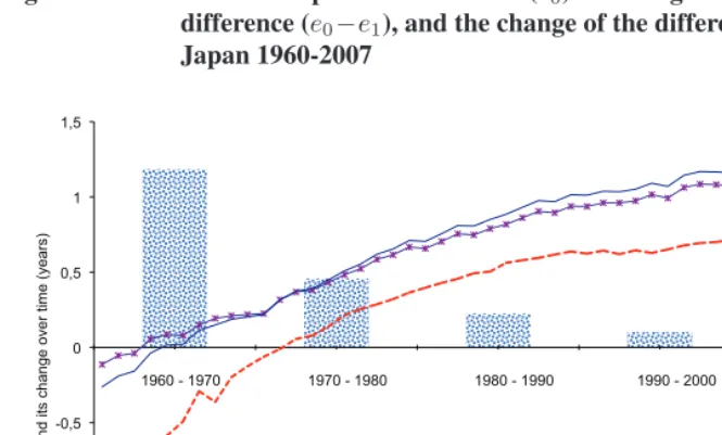
We further analyze the components of the change over time in the difference in life expectancies (at birth minus at age one). This difference in life expectancies is zero when the condition in equation 1 is fulfilled. Initially this difference is negative, but moves to positive values after the life table achieves a balanced situation. Figure 3a shows the life expectancies at birth and age one, their gap and the change per decade of this gap for Japanese males from 1960 to 2007.
The crossing in life expectancies for Japanese males occurs in 1971. This crossing occurred during a time that both measures were increasing from values of65.3and66.5
years fore0 and e1 respectively in 1960, to 79.2 and 78.4 in 2007 respectively. The
one year denoted in the figure as the bar of “Change ine0−e1”. However, the remaining
decades show a more modest reduction in the gap.
Figure 3a: Male life expectancies at birth (e0) and at age one (e1), their
difference (e0−e1), and the change of the difference by decade,
Japan 1960-2007
55 60 65 70 75 80
-1,5 -1 -0,5 0 0,5 1 1,5
1 11 21 31 41
e0
a
n
d
e1
Year
e0 -e1
a
n
d
i
ts
ch
a
n
g
e
o
ve
r
ti
me
(ye
a
rs)
Change in e0-e1
e0-e1
e1
e0
1960 - 1970 1970 - 1980 1980 - 1990 1990 - 2000 2000 - 2007
Source: Authors’ calculations based on the Human Mortality Database (2010).
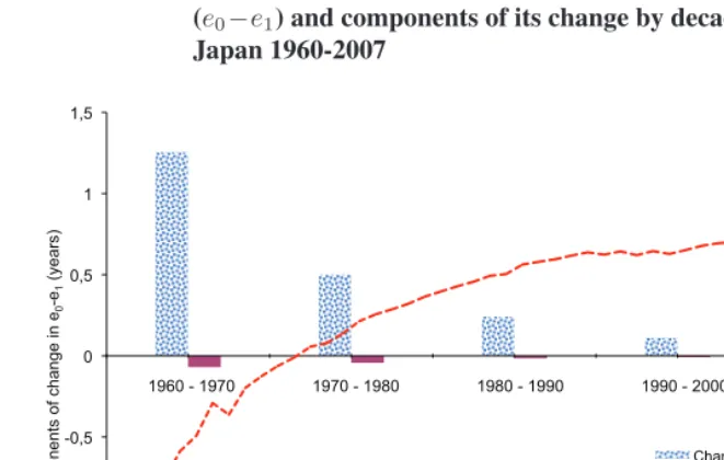
This change in the difference can be of further interest if the focus is on explaining trends over time in the gap between life expectancies at birth and at age one. In equation 2a, life expectancy at birth depends on three terms. Two components describe the mortality experience in the first year of life: probability of surviving to age one and person-years lived between birth and age one. The third term is life expectancy at age one which captures the experience of mortality after age one. The change in the difference between life expectancies is thus dependent on changes before and after age one. In the Appendix we propose a method to disentangle the changes in the gap over time due to reductions in mortality in the first year of life, and those due to reductions in mortality after age one. For notation in the Figures we refer to these as the “Change ine0−e1”
explained by “Changes below age one” and by “Changes above age one”. The top panel of Table 2 and Figure 3b show the components of change in the difference for Japanese males’ life expectancies for the decades between 1960 and 2007.
Figure 3b: Difference between male life expectancies at birth and at age one (e0−e1) and components of its change by decade,
Japan 1960-2007
-1,5 -1 -0,5 0 0,5 1 1,5
1 6 11 16 21 26 31 36 41 46
-1,5 -1 -0,5 0 0,5 1 1,5
e0
-
e1
Year
C
o
mp
o
n
e
n
ts
o
f
ch
a
n
g
e
i
n
e0 -e1
(ye
a
rs)
Changes below age one
Changes above age one
e0-e1
1960 - 1970 1970 - 1980 1980 - 1990 1990 - 2000 2000 - 2007
Source: Authors’ calculations based on the Human Mortality Database (2010).
for Japanese males is due mostly to great improvements in the first year of life. This can be observed in the high “Changes below age one” component. Below, we discuss the time trends for other populations with situations where the “Changes above age one” component is as important as the “Changes below age one” component.
4. Results
4.1 The crossover in industrialized countries
For industrialized countries, Table 1 and Figure 4 show the timing of the crossing ofe0
ande1. There is considerable variation in the timing of the crossover. Table 1 also shows
Figure 4: Life expectancy at birth at the year of the first crossing with life expectancy at age one, total population by country
BEL
BLR CZE FRG ESP
FRA
HUN ITA
LTU LUX
LVA NLD
NOR
NZL
POL PRT
SCO SVN
SWE
65 67 69 71 73 75 77
1955 1960 1965 1970 1975 1980 1985 1990 1995 2000 2005
L
if
e
e
xp
e
ct
a
n
cy
a
t
b
irt
h
&
a
t
a
g
e
o
n
e
(ye
a
rs)
Year ISL
CHE DNK
JPN
FIN TWN
CAN USA
EST BGR UKR
CHL
RUS ENW
AUT AUS
Source: Human Mortality Database (2010); Table 1 has the countries 3-letter codes.
The first crossing in the world occurred in 1957 for Icelandic females, for males in the same country this was not observed until 1967. The time of the male crossover is later than that of females for all analyzed countries except Slovenia. However, the variation in time is large with one year difference for Portugal, Russia and Spain, and14to18years difference in Latvia, Lithuania, Bulgaria and Ukraine. The crossings in life expectancies occurred in the range of infant mortality of11.6to14.5deaths per thousand live births for females and of13.6 to17.5for males. The level of life expectancy varied between the values of71.8to78.0years for females and58.9to72.3years for males. The larger variation in levels of life expectancy among males than among females (13.4versus6.2
The clear clusters of life expectancy at the time of the crossing observed in Figure 4, are not replicated for infant mortality. For example, Danish females have the highest infant mortality of any of the females’ values, even when their life expectancy was at a middle level at the crossing. Clearly mortality at ages other than the first year of life have a role in determining the time of the crossing. To further explain the crossing in life expectancies we look in detail at the interplay between the components of equation 1.
The decomposition of the change over time in the difference between life expectancy at birth minus life expectancy at age one allows study of the components of this change (see Appendix for details on the decomposition). The components have been aggregated into those that correspond to “Changes below age one” and “Changes above age one”. Across countries included in the HMD, the changes observed in the two components are clustered into three types:
(1) a decline in both components over time,
(2) fluctuations over time with an apparent declining trend but interrupted by mortality crises, and finally
(3) a bell shape trend with a peak in one of the periods and decline thereafter.
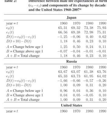
Table 2 and Figures 3b, 5a and 5b present the trends in the life expectancy difference, e0−e1, and components of its change during each of the decades since the 1960s up to
the first years of the 2000s for males (for Japan in Figure 3b, Russia in Figure 5a and the United States in Figure 5b). The selected countries represent the three types of changes mentioned above: Japan for (1), Russia for (2) and USA for (3).
Table 2: Difference between male life expectancies at birth and at age one (e0−e1) and components of its change by decade for Japan, Russia
and the United States 1960-2007*
Japan
year =t 1960 1970 1980 1990 2000 2007
e0(t) 65,31 69,32 73,38 75,93 77,70 79,20
e1(t) 66,56 69,38 72,98 75,31 76,97 78,42
D(t) =e0(t)−e1(t) −1,25 −0,06 0,40 0,62 0,73 0,78
D(t+10)−D(t) 1,18 0,46 0,23 0,10 0,05
A= Change below age 1 1,25 0,50 0,24 0,11 0,06 B= Change above age 1 −0,07 −0,04 −0,01 −0,01 0,00 A+B= Total change 1,18 0,46 0,23 0,10 0,05
Russia
year =t 1960 1970 1980 1990 2000 2008
e0(t) 63,67 63,07 61,38 63,76 58,99 61,79
e1(t) 65,33 63,73 61,95 64,02 59,04 61,39
D(t) =e0(t)−e1(t) −1,66 −0,66 −0,57 −0,26 −0,06 0,40
D(t+10)−D(t) 1,00 0,09 0,31 0,20 0,45
A= Change below age 1 0,96 0,04 0,36 0,10 0,48 B= Change above age 1 0,04 0,05 −0,05 0,10 −0,02 A+B= Total change 1,00 0,09 0,31 0,20 0,45
United States
year =t 1960 1970 1980 1990 2000 2006
e0(t) 66,63 67,02 69,99 71,87 74,28 75,50
e1(t) 67,66 67,62 69,98 71,64 73,86 75,06
D(t) =e0(t)−e1(t) −1,03 −0,60 0,00 0,23 0,42 0,44
D(t+10)−D(t) 0,44 0,60 0,22 0,19 0,02
A= Change below age 1 0,43 0,65 0,24 0,21 0,03 B= Change above age 1 0,00 −0,04 −0,02 −0,02 −0,01 A+B= Total change 0,44 0,60 0,22 0,19 0,02
Source: Human Mortality Database (2010).
Figure 5a: Difference between male life expectancies at birth and at age one (e0−e1) and components of its change by decade, Russia 1960-2008
-1,5 -1 -0,5 0 0,5 1 1,5
1 6 11 16 21 26 31 36 41 46
-1,5 -1 -0,5 0 0,5 1 1,5 e0 - e1 Year C o mp o n e n ts o f ch a n g e i n e0 -e1 (ye a rs)
Changes below age one
Changes above age one
e0-e1
1960 - 1970 1970 - 1980 1980 - 1990 1990 - 2000 2000 - 2008
Figure 5b: Difference between male life expectancies at birth and at age one (e0−e1) and components of its change by decade,
United States 1960-2006
-1,5 -1 -0,5 0 0,5 1 1,5
1 6 11 16 21 26 31 36 41 46
-1,5 -1 -0,5 0 0,5 1 1,5 e0 - e1 Year C o mp o n e n ts o f ch a n g e i n e0 - e1 (ye a rs)
Changes below age one Changes above age one
e0-e1
1960 - 1970 1970 - 1980 1980 - 1990 1990 - 2000 2000 - 2006
Figure 6: Infant mortality rate and life expectancy at birth for countries members of the WHO and UN, and not included in the HMD, latest available information from WHO and UN
10 20 30 40 50 60 70 80
0 20 40 60 80 100 120 140 160 180
L
if
e
e
xp
e
ct
a
n
cy
a
t
b
irt
h
(ye
a
rs)
Infant mortality rate (per 1000)
Life expectancy crossing (e0=e1)
AFRICA
AMERICA
ASIA
EUROPE
Source: United Nations (2008) and World Health Organization (2008).
4.2 The crossover in countries of the world
The United Nations (2008) and the World Health Organization (2008) databases can be used to present the recent situation of the world with respect to the crossing in life expectancies and the imbalance in life tables. Figure 6 presents the situation of the countries of the world in 2005 with respect to their life expectancy at birth and infant mortality. Four regions of the world are included in Figure 6, according to the United Nations macro regions: Africa, America, Asia/Oceania, and Europe. Also included is the line in where life expectancy at age one is equal to the inverse of infant mortality, as expressed in equation 1.
Asia/Oceania and the Americas have some of their countries still experiencing the imbalance in life tables while in others life expectancy at birth has the higher value. Although this plot presents the current situation, it cannot be reliably used to extrapolate possible crossing times and levels of mortality. As shown in Figure 3b for Russia, unexpected retrocession in mortality can delay or accelerate the crossing of the two life expectancies.
The countries included in the HMD have been excluded from Figure 6a, but a comparison using results from Table 1 and Figure 4 is instructive. The life expectancy crossing occurred between the levels of 65 to 75 years for countries included in the HMD. For countries in Figure 6 experiencing the crossing in recent years, this occurs in some cases at levels of life expectancy higher than75years. The interplay between levels of mortality below and above age one have caused these high life expectancies at the crossing. For example, in Figure 4 Southern Europe had the highest levels of life expectancy at the crossing. In these countries, life expectancy at age one had reached high levels as a consequence of high survivorship once the first year of life had passed. Infant mortality had also reduced, but it had to reach very low values to trigger the crossing. Similar circumstances were likely present in countries, such as those in Figure 6, where the crossing was experienced at levels of life expectancies above age75.
4.3 The imbalance in the life tables for the black and white populations of the USA
The black-white life expectancy gap in the USA can also be studied in terms of the imbalance in the life tables. Period life tables by race and sex for the USA since 1968 are used to study the crossover in life expectancies. As observed in Figure 7a, the trend for all the groups has been an increase in life expectancy and decline in infant mortality over time. All groups have moved from right to left in Figure 7a from high infant mortality to lower levels. The timing of the crossing in the white population was 1974 for females and 1977 for males. This can be observed in Figure 7a by noting that the values for the white population are mainly to the left of the line wheree0=e1 = 1/1m0. These years are
earlier than those shown in Table 1 for the USA population of 1977 for females and 1980 for males, where all races were combined. The female black population experienced this crossing in 1996 and black males are close to accomplishing this.
also found at older ages, as shown in Figure 7b, where the components of the change over time in the difference between life expectancies,e0−e1, of African American males are
examined.
Figure 7a: Infant mortality and life expectancy at birth for American females and males by race (white & black), 1968-2003
50 60 70 80
0 10 20 30 40 50
L
if
e
e
xp
e
ct
a
n
cy
a
t
b
irt
h
(ye
a
rs)
Infant mortality (per 1000)
White Females Black Females White Males Black Males
Life expectancy crossing (e0=e1)
1968 1968
1977 1974
1996
1968 1968
Source: BMDB(2010) and CDC (1984-2006).
Figure 7b: Difference between male life expectancies at birth and at age one (e0−e1) for the black American population and components of its
change for every five years, 1968-2003
-1,5 -1 -0,5 0 0,5 1 1,5
-1,5 -1 -0,5 0 0,5 1 1,5
e0
-
e1
Year
C
o
mp
o
n
e
n
ts
o
f
ch
a
n
g
e
i
n
e0
-
e1
(ye
a
rs)
Changes below age one
Changes above age one
e0-e1
1968 - 1975 1975 - 1980 1980 - 1985 1985 - 1990 1990 - 1995 1995 - 2000 2000 - 2003
Source: Author’s calculations based on BMDB(2010) and CDC (1984-2006).
5. Discussion
The motivation for this research was to find the relations among the functions of an imbalanced life table, i.e. when life expectancy at birth is lower than at age one,e0< e1.
This imbalance ends when e0 = e1. Equation 1 is a simple relation between infant
mortality and life expectancies at birth and age one and it is central to explicating the mechanisms of the crossover.
information on mortality is available, it is possible to analyze these disparities over time and region.
The illustration of the crossover in life expectancy observed in the HMD data suggests that socio-cultural, economic, and political factors that influence the intermediate factors that shape the mortality patterns in each country have traversed borders. In other words, the timing and mortality level at which populations progress from an imbalanced life table to a balanced one depend on the specific characteristics of each country, but also on regional characteristics. For example, the trends in mortality in the Baltic countries, Latvia and Lithuania, are very similar (Kasmel et al. 2004). Therefore, it is not surprising to find similar gaps between the female and male timing for the crossing in life expectancies (Table 1 and Figure 4). However, it is surprising to find these countries together with Bulgaria and Ukraine with the extreme of over14years difference between the female and male timing, while other eastern European countries only differ by a couple of years. Sex differentials in infant mortality vary widely across countries (Fuse and Crenshaw 2006). However, in the context of the Baltic countries this is probably not the only factor. The great disparity between females and males comes from a combination of infant mortality and high levels of adult male mortality. Furthermore, differentials among subpopulations within each country could also drive some of these results (Leinsalu, Vågerö, and Kunst 2004). It should be noted that in Estonia, the third Baltic country, females were close to a crossing in the 1970s, similar to the situation for the other two countries, and thus a similar gender gap in the timing of the crossing might have been observed.
declined before mortality in the first year of life, followed by a second phase of decline where mortality in infancy declined faster than in the later childhood years (Hill 1995). Life expectancy at age one captures the first type of reduction, and is independent of the level of mortality in the first year of life. In this setting, equation 1 suggests that infant mortality has to go down further to trigger the crossing.
The opposite situation is observed when a country achieves the crossing at an extremely low level of life expectancy–for example, the result for Russian males with a crossing at life expectancy of 59 years. Russian mortality in infancy and childhood, as well as in old age, was practically unaffected by the crisis in the 1990s, as opposed to the excess mortality among working age men (Leon, Shkolnikov, and McKee 2009). Another example of reversals in mortality is in the emergence of HIV/AIDS as a leading cause of adult mortality (Ahmad, Lopez, and Inoue 2000). The two life expectancies could be getting closer in highly affected countries, if infant mortality is not increasing as well.
The within-population comparison can also be used to contrast subgroup differences. Populations can be compared on how infant versus mortality after age one have changed. The black population in the USA lags behind its white counterpart not only on levels of survivorship but also on the timing of the crossover between life expectancies at birth and age one (see Figures 7a and 7b). This is partly due to the excess infant mortality still prevalent among blacks as compared with other races (Martin et al. 2005). It is also a consequence of the mortality levels at adult ages which have progressed and regressed with unexpected fluctuations (Harper et al. 2007). For example, the reduction in young adult mortality among black males in recent years will be causing a further delay in the life expectancy crossing unless it is accompanied by further reductions in infant mortality. Research is needed into the factors that have produced all the above mentioned trends. However, three corollaries can be extended from the results presented here:
• No single measure of mortality can fully describe the mortality situation of a population. An analysis of mortality changes or trends solely based on life expectancy at birth hides fundamental changes that might be occurring at specific ages. Analogously, an index of mortality for the first year of life without the context of mortality at other ages or an age-aggregated mortality measure of the population under study is also incomplete. The present analysis suggests that alternative indexes at different ages offer the possibility of an internal comparison of levels of mortality in the population under study. Relations between these complementary indexes, as those shown here, could help the study of possible excess mortality at certain ages. This is particularly important for developing countries that are still experiencing an imbalanced life table and for studies of historical trends in any population.
tables available in the Human Mortality Database (2010) are for the cohort born in 1915 which did not have a crossover in life expectancies for any country. In other words they have not achieved a minimum of infant mortality that corresponds to life expectancy at age one. Goldstein and Wachter (2006) have noted how period measures of mortality follow trends similar to cohort measures but lagged by some years. For example, the Swedish cohort of 1915 had a life expectancy of 66.37
years which was not observed until the period life table of 1939. We then would expect to observe the crossings in life expectancies, at birth and age one, earlier in the cohort life tables than in the period life tables. To explore this will necessitate waiting until persons from the cohorts born in the first half of the twentieth century have died.
• Finally, equation 1 can be generalized to older ages as shown in the Appendix for child mortality, but also for other ages. For example, in low mortality countries, neonatal rates of2deaths per thousand live births are not unusual (World Health Organization 2008). A neonatal rate is not a rate in terms of events over persons exposed (Preston, Heuveline, and Guillot 2001), but it can be transformed to a rate by changing the denominator into a measure of person-years lived. The neonatal rate is then approximately equal to a death rate of24deaths per thousand person-years. The inverse of this death rate is41.6, which is much lower than the current life expectancy at birth in low mortality countries (~80 years). Thus, from equation 2 it can then be concluded that life expectancy at age28days is higher than at age zero for populations with this level of neonatal mortality. This trend changes once the inverse of the neonatal rate is equal to life expectancies at birth and at age28days. More generally, life expectancies at birth and at age “x” are equal whene0=ex= 1/xm0, regardless of whether years, months or days are the
References
Ahmad, O., Lopez, A.D., and Inoue, M. (2000). The decline in child mortality: A reappraisal. Bulletin of the World Health Organization 10(78): 1175–1191.
doi:10.1590/S0042-96862000001000004.
Berkeley Mortality Database (2010). Berkeley mortality database. Berkeley, USA: University of California. Http://www.demog.berkeley.edu (4/02/2010).
Brass, W. (1971). On the scale of mortality. In: Brass, W. (ed.)Biological Aspects of Demography. London: Taylor & Francis.
Canudas-Romo, V. and Engelman, M. (2009). Maximum life expectancies: Revisiting the best practice trends.GenusLXV(1): 59–79.
Centers for Disease Control and Prevention (1984-2006). Vital statistics of the United States 1980, 1981, ..., 1995. National Vital Statistics Report 1996, 1997, ..., 2003. Http://www.cdc.gov/nchs/products/pubs/pubd/lftbls/lftbls.htm (13/01/2008).
Chiang, C.L. (1984).Life table and its applications. Malabar, Florida: Robert E. Krieger Publishing.
Coale, A.J. and Demeny, P. (1983). Regional model life tables and stable populations. New York: Academic Press, 2nd edition ed.
Cooper, R., Steinhauer, M., Schatzkin, A., and Miller, W. (1981). Improved mortality among u.s. blacks, 1968-1978: The role of antiracist struggle.International Journal of Health Services11(4): 511–522. doi:10.2190/WJEP-VB83-GAUT-XEJR.
Davis, K. (1945). The world demographic transition. Annals of the American Academy of Political and Social Science237(1): 1–11.doi:10.1177/000271624523700102. Dublin, L.I. (1923). The possibility of extending human life.Metron3(2): 175–197. Dublin, L.I. and Lotka, J.A. (1934). The history of longevity in the United States.Human
Biology6(1): 43–86.
Eblen, J.E. (1974). New estimates of the vital rates of the united states black population during the nineteenth century.Demography11(2): 301–320.doi:10.2307/2060565. Ewbank, D.C. (1987). History of black mortality and health before 1940. The Milbank
Quarterly, Currents of Health Policy: Impacts on Black Americans 65(1-Part 1): 100–128.doi:10.2307/3349953.
Frisbie, W.P., Song, S., Powers, D.A., and Street, J.A. (2004). The increasing racial disparity in infant mortality: Respiratory distress syndrome and other causes.
Demography41(4): 773–800. doi:10.1353/dem.2004.0030.
Fuse, K. and Crenshaw, E.M. (2006). Gender imbalance in infant mortality: A
cross-national study of social structure and female infanticide. Social Science & Medicine62(2): 360–374. doi:10.1016/j.socscimed.2005.06.006.
Galobardes, B., Lynch, J.W., and Smith, G.D. (2004). Childhood socioeconomic
circumstances and cause-specific mortality in adulthood: Systematic review and interpretation. Epidemiology Review26: 7–21.doi:10.1093/epirev/mxh008.
Goldstein, J.R. and Wachter, K.W. (2006). Relationships between period and
cohort life expectancy: Gaps and lags. Population Studies 60(3): 257–269.
doi:10.1080/00324720600895876.
Haines, M.R. (2003). Ethnic differences in demographic behavior in the United
States: Has there been convergence? Historical Methods 36(4): 157–195.
doi:10.1080/01615440309604818.
Harper, S., Lynch, J., Burris, S.J.D., and Smith, G.D. (2007). Trends in the black-white life expectancy gap in the United States, 1983-2003. The Journal of the American Medical Association297(11): 1224–1232. doi:10.1001/jama.297.11.1224.
Hill, K. (1995). The decline in childhood mortality. In: Simon, J.L. (ed.)The state of humanity. Boston: Blackwell: 30–36.
Horiuchi, S. (1991). Assessing the effects of mortality reduction on population ageing.
Population Bulletin of the United Nations31(2): 38–51.
Human Mortality Database (2010). Human mortality database. Berkeley, USA:
University of California, and Rostock, Germany: Max Planck Institute for
Demographic Research. Http://www.mortality.org (4/02/2010).
Hummer, R.A., Powers, D.A., Pullum, S.G., Gossman, G.L., and Frisbie, W.P. (2007). Paradox found (again): Infant mortality among the Mexican-origin population in the United States.Demography44(3): 441–457.doi:10.1353/dem.2007.0028.
Kannisto, V. (2001). Mode and dispersion of the length of life. Population: An English Selection13(1): 159–171.
Kasmel, A., Helasoja, V., Lipand, A., Prättälä, R., Klumbiene, J., and Pudule, I. (2004). Association between health behavior and self-reported health in Estonia, Finland, Latvia and Lithuania. The European Journal of Public Health14(1): 32–36.
doi:10.1093/eurpub/14.1.32.
Kintner, H.J. (2004). The life table. In: Siegel, J.S. and Swanson, D.A. (eds.)The methods and materials of demography, Second Edition. San Diego, USA: Elsevier Academic Press.
Kitagawa, E. (1955). Components of a difference between two rates. Journal of the American Statistical Association50(272): 1168–1194. doi:10.2307/2281213.
Klein, H.S. (2004). A population history of the United States. Cambridge, England: Cambridge University Press.
Kochanek, K.D., Maurer, J.D., and Rosenberg, H.M. (1994). Why did black life
expectancy decline from 1984 through 1989 in the United States? American Journal of Public Health84(6): 938–944. doi:10.2105/AJPH.84.6.938.
Kramer, M.S., Platt, R.W., Yang, H., Haglund, B., Cnattingius, S., and Berjso, P. (2002). Registration artifacts in international comparisons of infant mortality. Paediatric and Perinatal Epidemiology16: 16–22.
Lee, R. (2003). The demographic transition: Three centuries of fundamental
change. The Journal of Economic Perspectives 17(4): 167–190.
doi:10.1257/089533003772034943.
Leinsalu, M., Vågerö, D., and Kunst, A.E. (2004). Increasing ethnic differences in mortality in Estonia after the collapse of the Soviet Union. Journal of Epidemiology and Community Health58(7): 583–589.doi:10.1136/jech.2003.013755.
Leon, D.A., Shkolnikov, V.M., and McKee, M. (2009). Alcohol and Russian mortality: A continuing crisis.Addiction104: 1630–1636.doi:10.1111/j.1360-0443.2009.02655.x. Martin, J.A., Kochanek, K.D., Strobino, D.M., Guyer, B., and MacDorman, M.F. (2005). Annual summary of vital statistics 2003. Pediatrics 115(3): 619–634.
doi:10.1542/peds.2004-2695.
Murray, C.J.L., Ferguson, B.D., Lopez, A.D., Guillot, M., Salomon, J.A., and Ahmad, O. (2003). Modified logit life table system: Principles, empirical validation, and application.Population Studies57(2): 165–182. doi:10.1080/0032472032000097083. Notestein, F.W. (1945). Population - the long view. In: Schultz, T.W. (ed.)Food for the
Oeppen, J. and Vaupel, J.W. (2002). Broken limits to life expectancy.Science296(5570): 1029–1031.doi:10.1126/science.1069675.
Omran, A.R. (1971). The epidemiologic transition: A theory of the epidemiology of population change. Milbank Memorial Fund quarterly journal 49(4): 509–538.
doi:10.2307/3349375.
Preston, S.H., Heuveline, P., and Guillot, M. (2001). Demography: Measuring and modeling population processes. Malden, Mass: Blackwell Publishers.
Riley, J.C. (2005). The timing and pace of health transitions around the world.Population and Development Review31(4): 741–764. doi:10.1111/j.1728-4457.2005.00096.x. Robine, J.M. (2001). Redefining the stages of the epidemiological transition by a study
of the dispersion of life spans: The case of France. Population: An English Selection
13(1): 173–194.
Robine, J.M. (2006). Research issues on human longevity. In: Robine, J.M., Crimmins, E., Horiuchi, S., and Yi, Z. (eds.)Human longevity, individual life duration and the growth of the oldest-old population. Netherlands: Springer, International Studies in Population: 7–42.
United Nations (1982). Model life tables for developing countries. New York: United Nations, (sales no. e.81.xiii.7) ed.
United Nations (2008). Social indicators database. New York: United Nations.
Http://unstats.un.org/unsd/demographic/products/socind/health.htm (13/01/2008).
Vallin, J. and Meslé, F. (2009). The segmented trend line of highest
life expectancies. Population and Development Review 35(1): 159–187.
doi:10.1111/j.1728-4457.2009.00264.x.
Vaupel, J.W. and Canudas-Romo, V. (2002). Decomposing demographic change
into direct vs. compositional components. Demographic Research 7(1): 1–14.
doi:10.4054/DemRes.2002.7.1.
Vaupel, J.W. and Canudas-Romo, V. (2003). Decomposing change in life expectancy: A bouquet of formulas in honor of Nathan Keyfitz’s 90th birthday. Demography40(2): 201–216.doi:10.1353/dem.2003.0018.
Verna, M.K. and Smith, D.P. (1988). The current differential in black and white life expectancy.Demography25(4): 625–632. doi:10.2307/2061326.
Wilmoth, J.R. (1997). In search of limits. In: Wachter, K.W. and Finch, C.E. (eds.)
Between Zeus and the Salmon. The biodemography of longevity. Washington, D.C.: National Academy Press.
Wilmoth, J.R. (2000). Demography of longevity: Past, present and
future trends. Experimental Gerontology 35(9-10): 1111–1129.
doi:10.1016/S0531-5565(00)00194-7.
Wilmoth, J.R., Canudas-Romo, V., Zureick, S., Inoue, M., and Sawyer, C. (2009). Comparison of the un and who relational mortality models. In: Paper presented at the Population Association of America meeting. Detroit, MI, April 30 - May 2, 2009. World Health Organization (2008). World health statistics. World Health Organization.
Appendix
i) Formal proof of relation 2a in the text:
Let the function describing the number of survivors at age xand at timetin a life table be denoted as`(x, t). Life expectancy at agexand timetis calculated in terms of the survival function as:
ex(t) = ω
R
x
`(a, t)da
`(x, t) , (A1)
whereωis the highest age attained by a member of the population. To simplify some of the equations presented below, let the radix of the life table be equal to one,`(0, t) = 1.
The relations in equations 1 and 2 can be derived by noting that life expectancy at birth is a function of the life expectancy at age one. From equation A1 for life expectancy at birth we have:
e0(t) = ω
Z
1
`(x, t)da+
1
Z
0
`(x, t)dx. (A2)
The first term on the right is the product of life expectancy at age one by the number of survivors at age one, the second term is the person-years lived between birth and age one, which represent the two terms of equation 2a in the text:
e0(t) =e1(t)[1−1d0(t)] +1L0(t). (A3)
ii) Proposal of how to decompose the change over time in the difference in life expectancies
Let∆e0−1(t) =e0(t)−e1(t)denote the difference in life expectancies at birth and
at age one at timet, derived from subtractinge1 from equation A3. To disentangle the
share of the change that is due to mortality at young ages and the part due to mortality after age one, its change over time is decomposed. The change over time in∆e0−1can
be studied by calculating its derivative with respect to time (Vaupel and Canudas-Romo 2002; 2003). Let a dot on top of a variable denote the partial derivative with respect to time. Then we find that the change in the difference can be separated as:
˙
∆e0−1(t) =1L˙0−1d˙0(t)e1(t)−1d0(t) ˙e1(t). (A4)
The number of deaths before age one, 1d0(t), has declined over time and the number
of person years lived before age one,1L0(t), has increased. As a consequence, the first
two components will contribute to the positive increase of the difference. Opposed to this is the overall trend of increase in life expectancy at age one. Therefore, the third component of the change in life expectancy at age one opposes the increase in∆e0−1.
In some periods adult mortality increased, soe1 declined. As a consequence the third
component in equation A4 sometimes contributes positively to the increase in∆e0−1(for
example see Table 2 panel for Russia). In the text we refer to equation A4 as the “Change ine0−e1” explained by “Changes below age one”, and by “Changes above age one”.
If data are available for two points in time, denoted as t1 and t2, the relation in
equation A4 can be estimated using the decomposition of Kitagawa (1955) as
˙
∆e0−1(t) =
¡
1Lt02−1Lt01
¢
+¡1dt01−1dt02
¢ het1
1 +et12
2
i
+¡et1
1 −et12
¢ h1dt1
0 +1dt02
2
i
. (A5)
iii) Generalization of the life expectancy crossing
Crossings between life expectancies at birth and at ages above infancy have also occurred over time. Similar to equation 1, it is possible to obtain relations between life expectancies at birth and at other older ages. For example, the crossing with life expectancy at age five occurs at the time when the inverse of under five mortality is equal to life expectancy at age five, i.e.
e0=e5⇔ 1
5m0 =e5. (A6)
Figure 8 includes the timing of the crossing betweene0ande5for the HMD countries
Figure 8: Life expectancy at birth at the year of the first crossing with life expectancy at age five, total population by country
AUS AUT
CZE
ENW
ESP
FRA HUN
ISL
ITA
JPN NLD
NOR
PRT SVK
SWE
45 50 55 60 65 70
1900 1910 1920 1930 1940 1950 1960 1970 1980
L
if
e
e
xp
e
ct
a
n
cy
a
t
b
irt
h
&
a
t
a
g
e
f
ive
(ye
a
rs)
Year NZL
CHE
DNK CAN
SCO BEL
POL BGR
Source: Human Mortality Database (2010). See text for details of countries included. Table 1 has the countries 3-letter codes.
Several countries from the HMD have mortality series that start after the crossing between e0 ande5. For this reason we left out of Figure 8: Belarus, Chile, Estonia,