Application of linear combination between cubic B-spline collocation methods with different basis for solving the KdV equation

(1)

Application of linear combination between cubic B-spline

colloca-tion methods with different basis for solving the KdV equacolloca-tion

K. R. Raslan

Mathematics Department, Faculty of Science, Al-Azhar University, Nasr-City (11884), Cairo, Egypt. E-mail: kamal [email protected]

Talaat S. EL-Danaf

Mathematics Department, Faculty of Science, Menoufia University, Shebein El-Koom, Egypt. E-mail: [email protected]

Khalid K. Ali∗

Mathematics Department, Faculty of Science, Al-Azhar University, Nasr-City (11884), Cairo, Egypt. E-mail: [email protected]

Abstract In the present article, a numerical method is proposed for the numerical solution of the KdV equation by using a new approach by combining cubic B-spline functions. In this paper we convert the KdV equation to system of two equations. The method is shown to be unconditionally stable using von-Neumann technique. To test accuracy the error normsL2,L∞are computed. Three invariants of motion are predestined to determine the preservation properties of the problem and the numerical scheme leads to careful and active results. Furthermore, interaction of two and three solitary waves is shown. These results show that the technique introduced here is easy to apply.

Keywords. Collocation Method, cubic B-Spline methods, KdV equation.

2010 Mathematics Subject Classification. 65L05, 34K06, 34K28.

1. _Introduction

We will solve the KdV equation in this form [9]

ut+ε u ux+µ uxxx= 0, (1.1)

whereε, µare positive parameters and the subscriptsxandtdenote differentiation. The boundary conditions of (1.1) are given by.

u(a, t) =f1(a, t), u(b, t) =f2(b, t),

ux(a, t) =g1(a, t), ux(b, t) =g2(b, t), 0 ≤t≤T.

(1.2)

Received: 23 August 2016 ; Accepted: 20 December 2016.

∗Corresponding author.

(2)

And initial conditions of (1.1) are given by

u(x,0) =f(x),

ux(x,0) =f0(x) =g(x), a≤x≤b.

(1.3)

KdV equation is prototypical example of exactly solvable mathematical paradigm of waves on shallow water superficies. It grow for evolution, interaction of waves, and generation in physics. Due to the termut, (1.1) is called the evolution equation, the

nonlinear term causes the steepness of the wave, and the dispersive term defines the spreading of the wave. It is known that the influence of the steepness and spreading results in soliton solutions for the KdV equation.

The KdV equation is a one-dimensional nonlinear partial differential equation of third order, which plays a big role in the discussion of nonlinear dispersive waves. This equation was primarily derived by Korteweg-de Vries [4] to characterize the action of one dimensional shallow water solitary waves. Solitary waves are wave packets or pulses which diffuse in nonlinear dispersive media. For stable solitary wave solutions the nonlinear and dispersive terms in the KdV equation must equilibrium and in this status the KdV equation has wandering wave solutions called solitons. A soliton is a very particular type of solitary waves which save its waveform after inconsistency with other solitons. A small time solutions using a heat balance integral method to solve the KdV equation was gained by Kutluay et al. [9]. In their article, comprehensive comparisons with the analytical values over the acquaint interval are given. Bahadir [1] studied the exponential finite-difference technique to solve the KdV equation. This method has been shown to supply higher accuracy than the classical explicit finite difference and the heat balance integral method. Ozer and Kutluay [13] applied an analytical–numerical method, for solving the KdV equation and the obtained results are compared with that of the heat balance integral method and the corresponding analytical solution. Irk et al. [8] studied a second order spline approximation technique and made comparisons with earlier methods. Ozdes and Aksan [12] applied the method of lines for solving the KdV equation. A. Ozdes and E.N. Aksan [11] used a quadratic B-spline Galerkin finite element method and compared these techniques with the analytical solutions and other numerical solutions that are obtained earlier using various numerical techniques. O. Ersoy and I. Dag [7] applied the exponential cubic B-spline algorithm for solving the KdV equation. B. Saka [15] used cosine expansion-based differential quadrature method for numerical solution of the KdV equation. Dag and Y. Dereli [3] applied numerical solutions of KdV equation using radial basis functions. A. Canıvar et al. [2] applied A Taylor-galerkin finite element method for the KdV equation using cubic B-splines and also G. Micula and M. Micula [10] used on the numerical approach of Korteweg-de Vries-Burger equations by spline finite element and collocation methods.

(3)

the efficiency as well as the accuracy of the proposed method and we introduced the interaction of two and three solitary waves. Finally, conclusions are followed in section 6.

2. _{The kdv equation}

Now we can convert the Eq. (1.1) to system of equations as the following process: We takeux=vin the Eq. (1.1), so we get

ut+ε u ux+µ vxx= 0, ux=v,

(2.1)

whereε, µare positive parameters and the subscripts xandt denote differentiation. The boundary conditions of (2.1) are given by

u(a, t) =f1(a, t), u(b, t) =f2(b, t),

v(a, t) =g1(a, t), v(b, t) =g2(b, t), 0 ≤t≤T.

(2.2)

u(x,0) =f(x),

v(x,0) =g(x), a≤x≤b. (2.3)

3. Liner combination between cubic B-spline collocation method

To construct numerical solution, consider nodal points (xj, tn) defined in the region

[a, b]×[0, T], where

a=x0< x1< ... < xN =b, h=xj+1−xj = b−a

N , j= 0,1, ..., N,

0 =t0< t1< ... < tn< ... < T, tn =n∆t, n= 0,1, .... .

Through this section, linear combination between cubic B-splines (LCCBS) with dif-ferent basis functions is used to solve (2.1). The approximate solution, UN₍_{x, t}₎_,

VN₍_{x, t}_{) to the analytical solution}_u₍_{x, t}₎_{, v}₍_{x, t}₎_,_{in the form:}

UN(x, t) =

N+1 X

j=−1

cj(t)Lj(x), VN(x, t) = N+1

X

j=−1

δj(t)Lj(x), (3.1)

wherecj(t) and δj(t) are time-dependent unknowns to be determined and Lj(x) is

(LCCBS) basis functions as

(4)

whereC T Bj(x) the cubic trigonometric B-spline basis function at knots is given by

C T Bj(x) =

1 θ                   

ω3₍_x

j−2), xj−2≤x≤xj−1, ω(xj−2) (ω(xj−2)φ(xj) +ω(xj−1)φ(xj+1) )

+ω2₍_x

j−1)φ(xj+2), xj−1≤x≤xj ω(xj−2)φ2(xj+1) +φ(xj+2) (ω(xj−1)φ(xj+1)

+ω(xj)φ(xj+2)), xj−1≤x≤xj φ3₍_x

j+2), xj+1≤x≤xj+2,

0 otherwise ,

(3.2)

where ω(xj) = sin _x₋_x

j

2

, φ(xj) = sin _x

j−x

2

, θ = sin h 2

sin (h) sin 3h 2

and

Bj(x) is the exponential cubic B-spline basis functions at knots is are given by

Bj(x) =                        b2

(xj−2−x) −_p1(sinh (p(xj−2−x)))

, xj−2≤x≤xj−1

a1 + b1(xj−x) +c1 exp (p(xj−x))

+d1exp (−p(xj−x)) , xj−1≤x≤xj, a1 + b1(x−xj) +c1 exp (p(x−xj))

+d1exp (−p(x−xj)), xj≤x≤xj+1,

b2

(x−xj+2) −_p1(sinh (p(x−xj+2)))

, xj+1≤x≤xj+2 ,

0 otherwise ,

(3.3)

where

a1 = _{p h c}p h c₋_s, b1 =p₂

h _c_(c₋_1)+s2

(p h c−s)(1−c) i

,

b2 =_{2(p h c}p ₋_s), d1 =1₄

h_{exp (}₋_{p h) (1}₋_{c)+s(exp (}₋_{p h)}₋₁₎ (p h c−s)(1−c)

i ,

d2 = 1₄

h_{exp (p h) (1}₋_{c)+s(exp (p h)}₋₁₎ (p h c−s)(1−c)

i ,

s= sinh (p h), c=cosh (p h), h=b−a N .

The value of γ plays an important role in the (LCCBS) basis function. Ifγ = 0, the basis function is equal to cubic trigonometric B-spline basis function and ifγ= 1, the basis function is equal to exponential cubic B-spline basis functions. Hence, this work just considers the value of 0< γ <1.

(5)

ofUN(x), VN(x) and its two derivatives at the knots/nodes are determined in terms of the time parameterscj, δj as follows:

(U1)j= (U1) (xj) =a1cj−1+a2cj+a1cj+1,

(U0₎

j = (U0) (xj) =a3cj−1−a3cj+1,

(U00)_j= (U00) (xj) =a4cj−1+a5cj+a4cj+1

(V)_j= (V) (xj) =a1δj−1+a2δj+a1δj+1,

(V0)_j = (V0) (xj) =a3δj−1−a3δj+1,

(V00)_j= (V00) (xj) =a4δj−1+a5δj+a4δj+1,

(3.4)

where

a1=γ α1+ (1−γ)m1, a2=γ α2+ (1−γ), a3= (1−γ)m2−γ α3, a4=γ α4+ (1−γ)m3, a5=γ α5−2 (1−γ)m3,

m1=

(s−p h)

2(p h c−s), m2=

p(1−c)

2(p h c−s), m3= p

2_s

2(p h c−s),

α1= sin2 h₂ csc (h) csc 3h₂, α2= _{1+2 cos (h)}2 , α3=3₄ csc 3h₂,

α4=

3((1+3 cos (h)) csc2 ₍h 2))

16(2 cos(h

2)+cos(3h2))

, α5=−

3 cot2₍h 2)

2+4 cos (h),

4. _{Solution of kdv equation}

To apply the proposed method, we rewrite (2.1) as

∂u(x,t)

∂t +ε u(x, t) ∂u(x,t)

∂x +µ ∂2v(x,t)

∂x2 = 0,

∂u(x,t)

∂x =v(x, t).

(4.1)

We take the approximationsu(x, t) =Un

j andv(x, t) =Vjn, then from famous

Cranck-Nicolson scheme and forward finite difference approximation for the derivativet[5], we get

U_jn+1−U_jn

k +ε

(U Ux)n+1j +(U Ux)nj

2

+µ

(V)xxn+1j +(V)xxnj

2

= 0,

Uxn+1j +Uxnj

2

=V

n+1 j +V

n j

2 ,

(4.2)

wherek= ∆t is the time step.

The nonlinear terms in (4.2) is linearized using the form given by Rubin and Graves [14] as: we take linearization of the nonlinear term as follows:

(U Ux)n+1j =U n

jUxn+1j +U n+1

j Uxnj −U n

jUxnj. (4.3)

Using (3.4) and (4.3) in (4.2), we get a system of ordinary differential equations of the form:

A1cn+1j−1 +A2cn+1j +A3cn+1j+1 +A4δjn+1−1 +A5δjn+1+A4δn+1j+1 =

(6)

(4.4)

a3cn+1j−1 −a3cn+1j+1 −a1δn+1j−1 −a2δn+1j −a1δj+1n+1=

−a3cnj−1+a3cnj+1+a1δjn−1+a2δjn+a1δj+1n ,

(4.5)

where

A1=a1(1 +ε∆t₂ z2) +a3z1, A2=a2(1 +ε∆t₂ z2),

A3=a1(1 +ε∆t₂ z2)−a3z1, A4= µ₂∆ta4, A5= µ₂∆ta5.

The system thus obtained on simplifying (4.4) and (4.5) consists of (2N+ 2) lin-ear equations in the (2N+ 2) unknowns (c0,..., cN)T,(δ0,..., δN)T, which is the

tridiagonal system that can be solved by any algorithm.

4.1. Initial values. The initial vectors c0

j, δ0j can be obtained from the initial

con-dition and boundary values of the derivatives of the initial concon-dition as the following expressions:

UN₍_x

0,0) =f1(0), f or j= 0, UN₍_x

j,0) =f(xj), f or j= 1,2, . . . , N−1, UN₍_x

N,0) =f2(0), f or j=N, VN₍_x

0,0) =g1(0), f or j= 0, VN₍_x

j,0) =g(xj), f or j= 1,2, . . . , N−1, VN₍_x

N,0) =g2(0), f or j=N.

(4.6)

This yields a (2N+ 2)×(2N+ 2) system equations of the form

      

a2 2a1 0 0 · · · 0 0 0 a1 a2 a3 0 · · · 0 0 0

..

. ... ... ... ... ... ... ... 0 0 0 0 · · · a1 a2 a3

0 0 0 0 · · · 0 2a1 a2               c0 0 c0 1 .. . c0 N−1 c0_N

       =          

f1(x0) f(x0)

.. . .. .

f(xN) fN(x0)

          ,       

a2 2a1 0 0 · · · 0 0 0 a1 a2 a3 0 · · · 0 0 0

..

. ... ... ... ... ... ... ... 0 0 0 0 · · · a1 a2 a3

0 0 0 0 · · · 0 2a1 a2              

δ00 δ01

.. .

δ0 N−1 δ0 N        =          

g1(x0) g(x0)

.. . .. .

g(xN) gN(x0)

          , (4.7)

(7)

4.2. Stability analysis of the method. The stability analysis of nonlinear partial differential equations is not easy task to undertake. Most researchers copy with the problem by linearizing the partial differential equation. Our stability analysis will be based on the Von-Neumann concept in which the growth factor of a typical Fourier mode defined as

cn_j =Aζnexp(ijφ), δn

j =Bζnexp(ijφ),

(4.8)

g= ζ

n+1

ζn ,

where A and B are the harmonics amplitude, φ = k h , k is the mode number,

i = √−1 and g is the amplification factor of the schemes. We will be applied the stability of the schemes by assuming the nonlinear term as a constants λ. System (4.4) and (4.5) can be written as

a1cn+1j−1 +a2cn+1j +a1cn+1j+1 + λ k ε

2 a3c n+1

j−1−a3cn+1j+1

+

kµ 2 a4δ

n+1

j−1 +a5δn+1j +a4δj+1n+1

=a1cnj−1+a2cnj +a1cnj+1− λ k ε

2 a3c n

j−1−a3cnj+1

− kµ₂ a4δjn−1+a5δjn+a4δj+1n

,

(4.9)

a3cn+1j−1 −a3cn+1j+1 −a1δn+1j−1 −a2δn+1j −a1δj+1n+1=

−a3cnj−1+a3cnj+1+a1δnj−1+a2δnj +a1δj+1n .

(4.10)

Substituting (4.8) into the difference (4.9), we get

ζn+1hA(2a1cos(φ) +a2) + B kµ₂ (2a4cos(φ) +a5)−iλ k ε A a3sin (φ) i

=ζnh_A₍₂_a

1cos(φ) +a2)− B kµ₂ (2a4cos(φ) +a5) +iλ k ε A a3sin (φ) i

,

(4.11)

ζn+1 ζn =

h

A(2a1cos(φ) +a2)− B kµ₂ (2a4cos(φ) +a5) +iλ k ε A a3sin (φ) i

h

A(2a1cos(φ) +a2) + B kµ₂ (2a4cos(φ) +a5)−iλ k ε A a3sin (φ) i,

(4.12)

g= ζ

n+1

ζn =

X1+iY X2−iY

, (4.13)

where

(8)

Substituting (4.8) into the difference (4.10), we get

ζn+1_[₋_B ₍₂_a

1cos(φ) +a2)−2i A a3sin (φ)]

=ζn_[_B ₍₂_a

1cos(φ) +a2) + 2i A a3sin (φ)],

(4.14)

ζn+1 ζn =

[B (2a1cos(φ) +a2) + 2i A a3sin (φ)]

[−B (2a1cos(φ) +a2)−2i A a3sin (φ)]

, (4.15)

g= ζ

n+1

ζn =

X3+iZ X4−iZ

, (4.16)

where

X3=B (2a1cos(φ) +a2), X4=−B (2a1cos(φ) +a2), Z= 2A a3sin (φ).

From (4.13) and (4.16) we get|g| ≤1,hence the schemes are unconditionally stable. It means that there is no restriction on the grid size, i.e. onhand ∆t, but we should choose them in such a way that the accuracy of the scheme is not degraded.

5. _{Numerical testes and results of kdv equation}

In this section, we present numerical example to test validity of our scheme for solving KdV equation.

The norms L2-norm and L∞-norm are used to compare the numerical solution

with the analytical solution [6].

L2=

uE−uN =

q

hPN_i=0(uE

j −uNj )2, L∞= max

j

uE_j −uN_j

, j = 0, 1,· · ·, N,

(5.1)

whereuE _{is the exact solution}_u_and_uN _{is the approximation solution}_U

N,and the

quantitiesI1, I2 andI3 are shown to measure conservation for the schemes.

I1=R

∞

−∞u(x, t)dx∼=h

PN j=0(U)

n j , I2=

R∞

−∞ u(x, t)

2

dx∼=hPN_j=0 U2n j ,

I3= R∞

−∞

u(x, t)3₋3µ

εux(x, t) 2

dx∼= hPN_j=0h U3n j −

3µ ε U

2 x

n j

i ,

(5.2)

(9)

Test problem

We assume that the solution of the KdV equation is negligible outside the interval [a, b],together with all itsxderivatives tend to zero at the boundaries. Therefore, in our numerical study we replace Eq. (1.1) as shown in section 2 by

ut+ε u ux+µ vxx= 0, ux=v,

(5.3)

whereε, µare positive parameters and the subscripts xandt denote differentiation. The boundary conditions of (5.3) are given by

u(a, t) = 0, u(b, t) = 0,

v(a, t) = 0, v(b, t) = 0, 0 ≤t≤T. (5.4)

u(x,0) =f(x),

v(x,0) =g(x), a≤x≤b. (5.5)

Then the exact solutions of system (5.5) is

u(x, t) = 3c sech2(A x−B t+D), (5.6)

whereA= 1₂q3c_µ, B=ε c A.

This solution represents propagation of single soliton, having velocityε cand am-plitude 3c.

To investigate the performance of the proposed schemes we consider solving the following problem.

5.1. Single soliton. In previous section, we have provided modified exponential cu-bic B-spline schemes for the KdV equation, and we can take the following initial condition.

u(x,0) = 3c sech2(A x+D), (5.7)

whereA= 1₂q3c_µ.

The normsL2andL∞are used to compare the numerical results with the analytical

values and the quantities I1, I2 and I3 are shown to measure conservation for the

schemes.

Now, for comparison, we consider a test problem where,k= 0.005, D=−6, c= 0.3, ε= 1, µ= 4.84×10−4_{, p}_{= 1}_.₆₄_×₁₀−5_{, a}_{= 0}_{, b}_{= 2. The invariant}_I

1, I2andI3

changed by less than 1.62×10−4_, ₄_×₁₀−6_{and 1}_.₄₇₁_×₁₀−4_{respectively. Errors, also,}

at time 2 are satisfactorily smallL2-error =3×10−3 andL∞-error = 9 ×10−3 in the

computer program for the scheme atγ= 0.9 . The invariantI1, I2andI3changed by

(10)

program for the scheme atγ= 0.5. The invariantI1changed by less than 5.8×10−5,I2

approach to zero andI3changed by less than 2.05×10−5in the computer program for

the scheme atγ= 0.001. Our results are recorded in Table 1. The motion of solitary wave using our scheme is plotted at timest = 0,1,1.5,2,2.5, 3 in Figure 1. These results illustrate that the scheme has a highest accuracy and best conservation at

γ= 0.001 than other scheme at γ= 0.9, γ= 0.5. So we use the scheme atγ= 0.001 to study the motion of single solitary waves and interaction between two and three solitons.

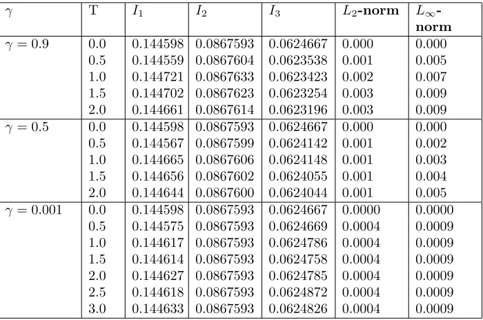
Table 1. Invariants and errors for single solitary wave k = 0.005, D=−6, p= 1.64×10−5_{, ε}_{= 1}_{, c}_{= 0}_.₃_{, µ}_{= 4}_.₈₄_×₁₀−4_{, a}₌

0, b= 2.

γ T I1 I2 I3 L2-norm L∞

-norm γ= 0.9 0.0

0.5 1.0 1.5 2.0 0.144598 0.144559 0.144721 0.144702 0.144661 0.0867593 0.0867604 0.0867633 0.0867623 0.0867614 0.0624667 0.0623538 0.0623423 0.0623254 0.0623196 0.000 0.001 0.002 0.003 0.003 0.000 0.005 0.007 0.009 0.009

γ= 0.5 0.0 0.5 1.0 1.5 2.0 0.144598 0.144567 0.144665 0.144656 0.144644 0.0867593 0.0867599 0.0867606 0.0867602 0.0867600 0.0624667 0.0624142 0.0624148 0.0624055 0.0624044 0.000 0.001 0.001 0.001 0.001 0.000 0.002 0.003 0.004 0.005

γ= 0.001 0.0 0.5 1.0 1.5 2.0 2.5 3.0 0.144598 0.144575 0.144617 0.144614 0.144627 0.144618 0.144633 0.0867593 0.0867593 0.0867593 0.0867593 0.0867593 0.0867593 0.0867593 0.0624667 0.0624669 0.0624786 0.0624758 0.0624785 0.0624872 0.0624826 0.0000 0.0004 0.0004 0.0004 0.0004 0.0004 0.0004 0.0000 0.0009 0.0009 0.0009 0.0009 0.0009 0.0009

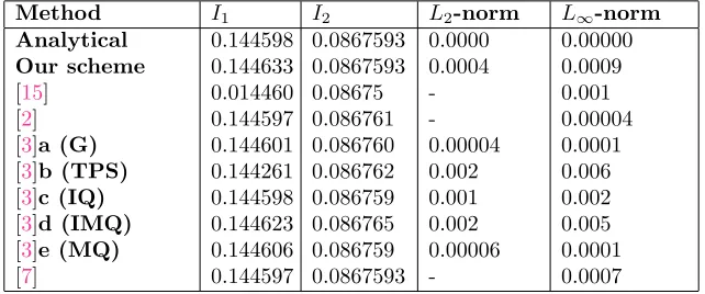
In the next table we make comparison between the results of our scheme and the results have been published in [15], [2], [3] and [7].

The results of our scheme are accurate than the results in [15], [3]b, [3]c and [3]d and related with the results in [3]a, [3]e and [7] and not better than the results in [2].

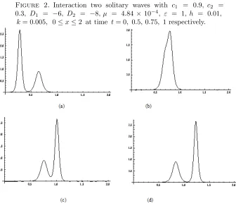
5.2. Interaction of two solitary waves. The interaction of two solitary waves having different amplitudes and traveling in the same direction is illustrated. We consider KdV equation with initial conditions given by the linear sum of two well separated solitary waves of various amplitudes

(11)

Figure 1. Single solitary wave with k= 0.005, D=−6, ε= 1, c=

0.3, µ = 4.84×10−4_{, γ} _{= 0}_.₀₀₁_, ₀ _≤ _x _≤ ₂_{, t} _{= 0}_,₁_,₁_.₅_,₂_,₂_.₅_,₃

respectively.

Table 2. Invariants and errors for single solitary wavek = 0.005, D = −6, ε = 1, c = 0.3, p = 1.64×10−5, γ = 0.001, µ = 4.84×10−4, 0≤x≤2, t= 3.

Method I1 I2 L2-norm L∞-norm

Analytical Our scheme

[15] [2] [3]a (G)

[3]b (TPS)

[3]c (IQ)

[3]d (IMQ)

[3]e (MQ)

[7]

0.144598 0.144633 0.014460 0.144597 0.144601 0.144261 0.144598 0.144623 0.144606 0.144597

0.0867593 0.0867593 0.08675 0.086761 0.086760 0.086762 0.086759 0.086765 0.086759 0.0867593

0.0000 0.0004 -0.00004 0.002 0.001 0.002 0.00006

-0.00000 0.0009 0.001 0.00004 0.0001 0.006 0.002 0.005 0.0001 0.0007

where A = 1₂

q_3c

j

µ , j = 1,2, 3, cj and Dj are arbitrary constants. In our

com-putational work. Now, we choose c1 = 0.9, c2 = 0.3, D1 = −6, D2 = −8, µ =

4.84×10−4, ε= 1, h= 0.01, k= 0.005 with interval [0, 2]. In Figure 3, the interac-tions of these solitary waves are plotted at different time levels.

(12)

Figure 2. Interaction two solitary waves with c1 = 0.9, c2 =

0.3, D1 = −6, D2 = −8, µ = 4.84 ×10−4, ε = 1, h = 0.01, k= 0.005, 0≤x≤2 at time t= 0, 0.5, 0.75, 1 respectively.

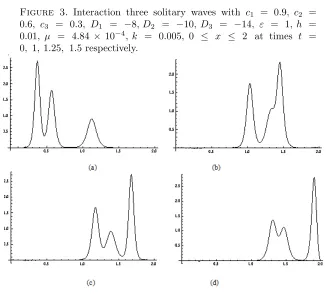
well separated solitary waves of various amplitudes

u(x,0) = 3cj sech2(A x+Dj), (5.9)

where A= 1₂q3cj

µ , j = 1,2, 3, −cj and Dj are arbitrary constants. In our

com-putational work. Now, we choose c1 = 0.9, c2 = 0.6, c3 = 0.3, D1 = −8, D2 =

−10, D3=−14, ε= 1, h= 0.01, µ= 4.84×10−4, k= 0.005 with interval [0, 2]. In

Figure 4 the interactions of these solitary waves are plotted at different time levels.

6. _Conclusion

(13)

Figure 3. Interaction three solitary waves with c1 = 0.9, c2 =

0.6, c3 = 0.3, D1 = −8, D2 = −10, D3 = −14, ε = 1, h =

0.01, µ = 4.84 ×10−4_{, k} _{= 0}_.₀₀₅_, ₀ _≤ _x _≤ _{2 at times} _t ₌

0, 1, 1.25, 1.5 respectively.

References

[1] A.R. Bahadir, Exponential finite-difference method applied to Korteweg-de Vries equation for small times, Appl. Math. Comput., 160 (2005), 675–682.

[2] A. Canıvar, M. Sari, and I. Dag, A Taylor-Galerkin finite element method for the KdV equation using cubic B-splines, Physica B: Condensed Matter, 405(16) 2010, 3376–3383.

[3] I. Dag and Y. Dereli, Numerical solutions of KdV equation using radial basis functions, Applied Mathematical Modelling, 32(4) (2008), 535–546.

[4] P.G. Drazin and R.S. Johnson, Solitons: an introduction, Cambridge University press, 1989. [5] T. S. EL-Danaf, K. R. Raslan and Khalid K. Ali, Collocation method with cubic B- splines for

solving the generalized regularized long wave equation, Int. J. of Num. Meth. and Appl., 15(1) (2016), 39–59.

[6] T. S. EL-Danaf, K. R. Raslan and Khalid K. Ali, New numerical treatment for the generalized regularized long wave equation based on finite difference scheme, Int. J. of S. Comp. and Eng. (IJSCE)’, 4 (2014), 16–24.

[7] O. Ersoy and I. Dag, The exponential cubic B-spline algorithm for Korteweg- de Vries equation, Advances in Numerical Analysis, 2015 (2015), 8 pages. DOI 10.1155/2015/367056.

[8] D. Irk, I. Dag and B. Saka, A small time solutions for the Kortewegde Vries equation using spline approximation, Appl. Math. Comput., 173 (2006), 834–846.

(14)

[10] G. Micula and M. Micula, On the numerical approach of Korteweg-de Vries- Burger equations by spline finite element and collocation methods, Seminar on Fixed PointTheory Cluj- Napoca, 3 (2002), 261–270.

[11] A. Ozdes and E.N. Aksan, Numerical solution of Korteweg-de Vries equation by Galerkin B-spline finite element metho, Appl. Math. Comput., 175 (2006), 1256– 1265.

[12] A. Ozdes and E.N. Aksan, The method of lines solution of the Korteweg-de Vries equation for small times, Int. J. Contemp. Math. Sci., 1(13) (2006), 639–650.

[13] S. Ozer and S. Kutluay, An analytical–numerical method for solving the Korteweg- de Vries equation, Appl. Math. Comput., 164 (2005), 789–797.

[14] S.G. Rubin, R.A. Graves, A cubic spline approximation for problems in fluid mecha- nics, Nasa TR R-436, Washington, D.C., 1975.