in the population sciences published by the Max Planck Institute for Demographic Research Konrad-Zuse Str. 1, D-18057 Rostock·GERMANY www.demographic-research.org
DEMOGRAPHIC RESEARCH
VOLUME 15, ARTICLE 9, PAGES 289-310
PUBLISHED 20 OCTOBER 2006
http://www.demographic-research.org/Volumes/Vol15/9/ DOI: 10.4054/DemRes.2006.15.9
Research Article
Lee-Carter mortality forecasting:
a multi-country comparison
of variants and extensions
Heather Booth
Rob J. Hyndman
Leonie Tickle
Piet de Jong
c
°2006 Booth et al.
This open-access work is published under the terms of the Creative Commons Attribution NonCommercial License 2.0 Germany, which permits use, reproduction & distribution in any medium for non-commercial purposes, provided the original author(s) and source are given credit.
1 Introduction 290
2 The five methods 291
2.1 The Lee-Carter method 291
2.2 The Lee-Miller variant 292
2.3 The Booth-Maindonald-Smith variant 293
2.4 The Hyndman-Ullah functional data method 293
2.5 The De Jong-Tickle LC(smooth) method 294
3 Data and accuracy measures 295
4 Forecast evaluation of the five methods 296
5 Decomposition of differences among the three LC variants 301
6 Discussion and conclusions 304
7 Acknowledgments 307
Lee-Carter mortality forecasting:
a multi-country comparison of variants and extensions
Heather Booth1
Rob J. Hyndman2
Leonie Tickle3
Piet de Jong4
Abstract
We compare the short- to medium-term accuracy of five variants or extensions of the Lee-Carter method for mortality forecasting. These include the original Lee-Carter, the Lee-Miller and Booth-Maindonald-Smith variants, and the more flexible Hyndman-Ullah and De Jong-Tickle extensions. These methods are compared by applying them to sexspe-cific populations of 10 developed countries using data for 1986-2000 for evaluation. All variants and extensions are more accurate than the original Lee-Carter method for fore-casting log death rates, by up to 61%. However, accuracy in log death rates does not necessarily translate into accuracy in life expectancy. There are no significant differences among the five methods in forecast accuracy for life expectancy.
1Demography and Sociology Program, Research School of Social Sciences, Australian National University,
Canberra ACT 0200, Australia. Email: [email protected]
2Department of Econometrics and Business Statistics, Monash University.
Email: [email protected]
1. Introduction
The future of human survival has attracted renewed interest in recent decades. The his-toric rise in life expectancy shows little sign of slowing, and increased survival is a sig-nificant contributor to population ageing. In this context, forecasting mortality has gained prominence. The future of mortality is of interest not only in its own right, but also in the context of population forecasting, on which economic, social and health planning is based. The future provision of health and social security for ageing populations is now a central concern of countries throughout the developed world.
This renewed interest in mortality forecasting has been accompanied by the devel-opment of new and more sophisticated methods; for a review, see Booth (2006). A sig-nificant milestone was the publication of the Lee-Carter method (Lee and Carter, 1992), although a principal components approach had previously been employed by Bell and Monsell (1991); see also Bell (1997). The Lee-Carter method is regarded as among the best currently available and has been widely applied (e.g., Lee and Tuljapurkar, 1994; Wilmoth, 1996; Tuljapurkar et al., 2000; Li et al., 2004; Lundström and Qvist, 2004; Buettner and Zlotnik, 2005). The Lee-Carter method was a significant departure from previous approaches: in particular it involves a two-factor (age and time) model and uses matrix decomposition to extract a single time-varying index of the level of mortality, which is then forecast using a time series model. The strengths of the method are its simplicity and robustness in the context of linear trends in age-specific death rates. While other methods have subsequently been developed (e.g., Brouhns et al., 2002; Renshaw and Haberman, 2003a,b; Currie et al., 2004; Bongaarts, 2005; Girosi and King, 2006), the Lee-Carter method is often taken as the point of reference.
The underlying principle of the Lee-Carter method is the extrapolation of past trends. The method was designed for long-term forecasting based on a lengthy time series of historic data. However, significant structural changes have occurred in mortality patterns over the twentieth century, reducing the validity of experience in the more distant past for present forecasts. Thus, judgement is inevitably involved in determining the appropriate fitting period. If a longer fitting period is not advantageous, the heavy data demands of the Lee-Carter method can be somewhat relaxed. Whether length of fitting period significantly affects forecast accuracy has not been systematically evaluated.
Indeed, evaluation is limited by the lengthy forecast horizon. However, the forecast can be evaluated in the shorter term using historical data to evaluate out-of-sample fore-casts. Shorter term evaluation is relevant to the increasing number of applications that adopt the Lee-Carter method for short- to medium-term forecasting. Shorter term evalu-ation also informs the longer term prospects of the forecast because errors in forecasting trends can be identified.
by Lee and Miller (2001) and the second by Booth et al. (2002). These three variants of the Lee-Carter method were first evaluated by Booth et al. (2005). In addition, there have been several extensions of the Lee-Carter method, retaining some of its flavour but adding additional statistical features such as non-parametric smoothing, Kalman filtering and multiple principal components. Two such extensions are by Hyndman and Ullah (2007) and De Jong and Tickle (2006). It is not known how these extensions perform compared with the Lee-Carter method and its variants.
This paper presents the results of an evaluation of these five mortality forecasting methods: Lee-Carter, Lee-Miller, Booth-Maindonald-Smith, Hyndman-Ullah and De Jong-Tickle. Each method is applied to data by sex for ten countries. The evalua-tion involves fitting the different methods to data up to 1985, forecasting for the period 1986–2000, and comparing the forecasts with actual mortality in that period. This paper does not address forecast uncertainty, which has been a recent research focus particularly in relation to long-term forecasting (see Lutz and Goldstein, 2004; Booth, 2006). Rather, it focuses on short- to medium-term forecast accuracy.
2. The five methods
2.1 The Lee-Carter method
The Lee-Carter method of mortality forecasting combines a demographic model of mor-tality with time-series methods of forecasting. The method is generally interpreted as making the use of the longest available time series of data. The Lee-Carter model of mortality is
lnmx,t=ax+bxkt+εx,t (1)
wheremx,t is the central death rate at age xin year t, kt is an index of the level of mortality at timet,axis the average pattern of mortality by age across years,bx is the relative speed of change at each age, andεx,t is the residual at age xand time t. The ax are calculated as the average oflnmx,t over time, and the bx andkt are estimated by singular value decomposition (Trefethen and Bau, 1997). Constraints are imposed to obtain a unique solution: theaxare set equal to the means over time of lnmx,tand the bxsum to 1; thektsum to zero.
The Lee-Carter method adjustsktby refitting to total observed deaths. This adjust-ment gives greater weight to ages at which deaths are high, thereby partly counterbalanc-ing the effect of uscounterbalanc-ing the logarithm of rates in the Lee-Carter model. The adjustedkt is extrapolated using ARIMA time series models (e.g., Makridakis et al., 1998). Lee and Carter used a random walk with drift model. The model is
wheredis the average annual change inkt, andetare uncorrelated errors. Lee and Carter used a dummy variable to take account of the outlier resulting from the 1918 influenza epidemic. Forecast age-specific death rates are obtained using extrapolatedktand fixed ax andbx. In this case, the jump-off rates (i.e., the rates in the last year of the fitting period or jump-off year) are fitted rates.
It should be noted that the Lee-Carter method does not prescribe the linear time series model of a random walk with drift for all situations. However, this model has been judged to be appropriate in almost all cases; even where a different model was indicated, the more complex model was found to give results which were only marginally different to the random walk with drift (Lee and Miller, 2001). Further, Tuljapurkar et al. (2000) found that the rate of decline in mortality was constant (i.e.,ktwas linear) for the G7 countries, reinforcing the use of a random walk with drift as an integral part of the Lee-Carter method.
2.2 The Lee-Miller variant
The Lee-Miller variant differs from this basic Lee-Carter method in three ways:
1 the fitting period is reduced to commence in 1950; 2 the adjustment ofktinvolves fitting toe(0)in yeart;
3 the jump-off rates are taken to be the actual rates in the jump-off year.
In their evaluation of the Lee-Carter method, Lee and Miller (2001) noted that for US data the forecast was biased when using the fitting period 1900–1989 to forecast the period 1990–1997. The main source of error was the mismatch between fitted rates for the last year of the fitting period (1989) and actual rates in that year; this jump-off error or bias amounted to 0.6 years in life expectancy for males and females combined (Lee and Miller, 2001, p.539). Jump-off bias was avoided by constraining the model such thatkt passes through zero in the jump-off year.
It was also noted that the pattern of change in mortality was not fixed over time, as the Lee-Carter model assumes. Based on different age patterns of change (orbxpatterns) for 1900–1950 and 1950–1995, Lee and Miller (2001) adopted 1950 as the first year of the fitting period. This solution to evolving age patterns of change had been adopted by Tuljapurkar et al. (2000).
2.3 The Booth-Maindonald-Smith variant
The Booth-Maindonald-Smith variant also differs from the Lee-Carter method in three ways:
1 the fitting period is chosen based on statistical goodness-of-fit criteria under the assumption of linearkt;
2 the adjustment ofktinvolves fitting to the age distribution of deaths;
3 the jump-off rates are taken to be the fitted rates based on this fitting methodology.
Booth et al. (2002) fitted the Lee-Carter model to Australian data for 1907–1999 and found that the ‘universal pattern’ (Tuljapurkar et al., 2000) of constant mortality decline as represented by linearktdid not hold over that fitting period. In addition, problems were encountered in meeting the assumption of constantbxin the underlying Lee-Carter model. Taking assumption of linearity inktas a starting point, the Booth-Maindonald-Smith variant seeks to maximize the fit of the overall model by restricting the fitting period to maximize fit to the linearity assumption, which also results in the assumption of constantbxbeing better met. The choice of fitting period is based on the ratio of the mean deviances of the fit of the underlying Lee-Carter model to the overall linear fit: this ratio is computed for all possible fitting periods (i.e., varying the starting year but holding the jump-off year fixed) and the chosen fitting period is that for which this ratio is substantially smaller than for periods starting in previous years.
The procedure for the adjustment ofktwas modified. Rather than fit to total deaths, Dt, the Booth-Maindonald-Smith variant fits to the age distribution of deaths,Dx,t, using the Poisson distribution to model the death process and the deviance statistic to measure goodness of fit (Booth et al., 2002). The jump-off rates are taken to be the fitted rates under this adjustment.
2.4 The Hyndman-Ullah functional data method
The approach of Hyndman and Ullah (2007) uses the functional data paradigm (Ramsay and Silverman, 2005) for modelling log death rates. It extends the Lee-Carter method in the following ways:
1 mortality is assumed to be a smooth function of age that is observed with error; smooth death rates are estimated using nonparametric smoothing methods; 2 more than one set of(kt, bx)components is used;
The Hyndman-Ullah approach can be expressed using the equation
lnmx,t=a(x) + J
X
j=1
kt,jbj(x) +et(x) +σt(x)εx,t (3)
wherea(x) is the average pattern of mortality by age across years, bj(x) is a “basis function” andkt,jis a time series coefficient. The use ofa(x)rather thanaxis intended to show thata(x)is a smooth function of age where age is a continuous quantity. It is estimated by applying penalized regression splines (Wood, 2000) to each year of data and averaging the results. The pairs (kt,j,bj(x)) forj = 1, . . . , Jare estimated using principal component decomposition. The error termσt(x)εx,taccounts for observational error that varies with age; i.e., it is the difference between the observed rates and the spline curves. The error termet(x)is modelling error; i.e., it is the difference between the spline curves and the fitted curves from the model.
In our implementation of the Hyndman-Ullah method, we do not use robust estima-tion. Rather, the fitting period is restricted to 1950 on, thus avoiding outliers. This was found to give slightly more accurate forecasts than using all the data with robust estima-tion. We useJ = 6for all data sets. The results seem relatively insensitive to the choice ofJ providedJ is large enough. We forecast the time series coefficientskt,j for each jusing damped Holt’s method based on the state space formulation of Hyndman et al. (2002).
2.5 The De Jong-Tickle LC(smooth) method
The approach of De Jong and Tickle (2006) uses the state space framework (Harvey, 1989) for modelling log death rates. State space models encompass a wide range of flex-ible multivariate time series models of which the Lee-Carter model is a special case. The general framework admits a host of specialisations and generalisations, and includes esti-mation of unknown parameters, inference, diagnostic checking and forecasting including forecast error calculations.
The Lee-Carter model (1) may be written in the form
yt=a+bkt+εt (4)
whereytis the vector of the log-central death rates at each age in yeart,aandbare vectors of the corresponding Lee-Carter parameters for each age,kt is an index of the level of mortality in yeartas in the Lee-Carter model, andεtis a vector of error terms at each age in yeart.
De Jong and Tickle (2006) developed the more general specification
whereX is a known “design” matrix with more rows than columns, unless X = I in which case the model reduces to (4). Model (5) addresses an issue with LC model (4) where there is anaand abparameter for each age, which means that thekttime series has an independent impact at each age. In model (5),Xhaving fewer columns than rows means that there are feweraandbparameters than there are age groups. The effects of thekttime series are not independent across age but are constrained by the structure of X, imposing across-age smoothness. The authors thus termed the model LC(smooth).
It is possible to include several time series components in which casektis a vector andbis a matrix with one column for each component ofkt. Various forms of the matrix X and the time seriesktare possible. In the current analysis, the matrixX is based on B-splines (Hastie and Tibshirani, 1990) which impose a quadratic form on log-mortality between knots at various ages. A single random walk with drift time series has been used. Maximum likelihood estimates of the model are derived using Kalman filtering and smoothing (Harvey, 1989). The aparameters are derived from the average of the rates in the jump-off year and the previous year, with the effect that the jump-off rates are smoothed average actual rates. As for Hyndman-Ullah, the fitting period is restricted to 1950 on to avoid outliers.
3. Data and accuracy measures
The data for this study are taken from the Human Mortality Database (2006). Ten coun-tries were selected giving 20 sex-specific populations for analysis. The ten councoun-tries se-lected are those with reliable data series commencing in 1921 or earlier. It was desirable to use only countries for which the available time series of data commenced somewhat ear-lier than 1950 in order to maintain the full and consistent comparison of the three variants. Lee and Carter (1992) used US data for the full period available, 1900–1989. Therefore this multi-country analysis uses data for the period commencing in 1900 where possible. Though for some countries the data extend back to the nineteenth century, these were truncated at 1900: the use of pre-1900 data would both reduce comparability of meth-ods across countries and necessitate a time series model with a non-linear trend which falls outside the scope of both applications to date and the current analysis. The selected countries are shown in Table 1 along with the dates used to define the fitting periods.
dif-Table 1: Start year for different countries and methods.
Country LC LM BMS [m] BMS [f] HU DJT
Australia 1921 1950 1968 1970 1950 1950
Canada 1921 1950 1974 1976 1950 1950
Denmark 1900 1950 1968 1967 1950 1950
England and Wales 1900 1950 1968 1972 1950 1950
Finland 1900 1950 1971 1971 1950 1950
France 1900 1950 1971 1969 1950 1950
Italy 1900 1950 1968 1968 1950 1950
Norway 1900 1950 1969 1963 1950 1950
Sweden 1900 1950 1976 1969 1950 1950
Switzerland 1900 1950 1962 1962 1950 1950
Note: The fitting period is defined by start year to 1985; the forecasting period is defined by 1986 to 2000.
fer from those used in previous work in that overseas World War II deaths have been excluded.
The five methods were fitted to periods ending in 1985 and used to forecast death rates from 1986 to 2000. The methods are evaluated by comparing forecast log death rates with actual log death rates.
Forecasting error in log death rates (forecast−actual) is averaged over forecast years, countries or ages to give different views of the relative bias of the five methods. The absolute errors are also averaged to provide measures of forecast accuracy. In addition to these errors in log death rates, the error in life expectancy(forecast−actual)is examined. Again, these (and the absolute errors) are averaged over countries or years to give different summary measures.
We investigate forecast bias in the methods usingt-tests of zero mean applied to the errors in log death rates averaged across forecast horizon and age. The sexes are treated separately. Similarly, we test for zero mean in the errors in life expectancy averaged across forecast horizon.
4. Forecast evaluation of the five methods
and HU show no evidence of bias in either female or male mortality. Sex differences in this measure are related to the cancellation of positive and negative errors (compare Table 3).
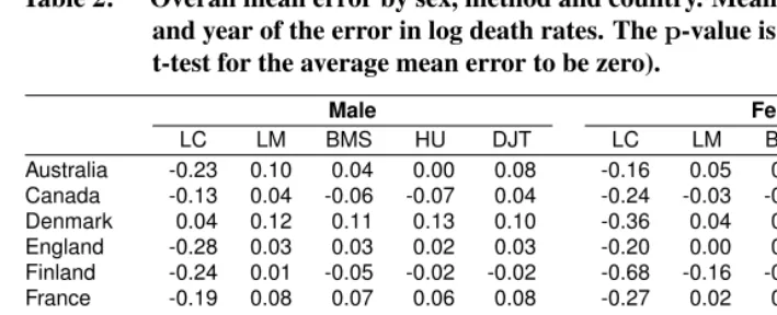
Table 2: Overall mean error by sex, method and country. Mean taken over age and year of the error in log death rates. Thep-value is a test of bias (a t-test for the average mean error to be zero).
Male Female
LC LM BMS HU DJT LC LM BMS HU DJT
Australia -0.23 0.10 0.04 0.00 0.08 -0.16 0.05 0.01 0.06 0.02
Canada -0.13 0.04 -0.06 -0.07 0.04 -0.24 -0.03 -0.07 -0.08 -0.05
Denmark 0.04 0.12 0.11 0.13 0.10 -0.36 0.04 0.03 0.03 0.02
England -0.28 0.03 0.03 0.02 0.03 -0.20 0.00 0.02 0.00 -0.02
Finland -0.24 0.01 -0.05 -0.02 -0.02 -0.68 -0.16 -0.17 -0.13 -0.17
France -0.19 0.08 0.07 0.06 0.08 -0.27 0.02 0.03 0.02 0.02
Italy -0.06 0.00 -0.03 0.02 0.01 -0.24 -0.06 -0.08 -0.05 -0.06
Norway 0.17 0.10 0.11 0.07 0.09 -0.57 0.00 -0.04 -0.01 -0.05
Sweden -0.09 0.06 -0.01 0.04 0.07 -0.61 -0.01 -0.04 -0.05 -0.03
Switzerland -0.12 0.02 0.02 0.06 0.02 -0.44 -0.02 -0.03 0.02 -0.03
Average -0.11 0.06 0.02 0.03 0.05 -0.38 -0.02 -0.03 -0.02 -0.03
p-value 0.03 0.00 0.27 0.09 0.00 0.00 0.43 0.12 0.34 0.08
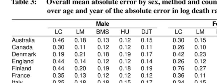
Table 3 provides a summary of forecast accuracy based on mean absolute error. Again, LC performs least well and there are only minor differences among the other four meth-ods. It is notable that the simple variations on the LC method used in LM and BMS pro-vide substantial improvements in forecast accuracy which are only marginally improved by the more sophisticated HU and DJT methods. It is also notable that for this abso-lute measure, female and male mortality are equally difficult to forecast. Some countries (notably the Nordic countries) proved more difficult to forecast than others.
We used a 2-way ANOVA model (with method and country as factors) on the mean absolute errors to test whether the methods are significantly different. A test for differ-ences between methods was highly significant (p < 0.001). However, using Tukey’s Honest Significant Differences to see which pairs of methods were different showed that the original LC method was significantly different from all other methods (p < 0.001), but the other four methods were not significantly different from each other (allp-values greater than 0.86).
Table 3: Overall mean absolute error by sex, method and country. Mean taken over age and year of the absolute error in log death rates.
Male Female
LC LM BMS HU DJT LC LM BMS HU DJT
Australia 0.46 0.18 0.13 0.12 0.15 0.30 0.15 0.12 0.12 0.11
Canada 0.30 0.11 0.12 0.12 0.11 0.26 0.10 0.12 0.11 0.09
Denmark 0.19 0.21 0.18 0.19 0.17 0.42 0.23 0.21 0.20 0.18
England 0.44 0.14 0.12 0.12 0.14 0.26 0.12 0.10 0.11 0.11
Finland 0.44 0.20 0.19 0.18 0.19 0.76 0.27 0.26 0.22 0.25
France 0.35 0.13 0.12 0.12 0.12 0.36 0.11 0.10 0.09 0.09
Italy 0.25 0.18 0.18 0.15 0.17 0.34 0.15 0.15 0.15 0.15
Norway 0.23 0.20 0.18 0.17 0.18 0.65 0.19 0.18 0.18 0.18
Sweden 0.24 0.20 0.16 0.17 0.17 0.67 0.18 0.18 0.16 0.14
Switzerland 0.25 0.18 0.16 0.15 0.15 0.50 0.20 0.18 0.15 0.15
Average 0.31 0.17 0.15 0.15 0.15 0.45 0.17 0.16 0.15 0.15
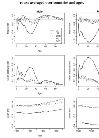
mean errors at the older ages. This is due to the fact that the longer LC fitting period produces estimates ofbxthat do not reflect the age pattern of change in the forecasting period. The dominance of the large negative errors at the younger ages accounts for the overall underestimation observed for LC in Table 2, and for males the greater cancellation of errors accounts for their less-biased forecasts.
Averages across age are shown over time in the lower half of Figure 1. All methods show similar trends in mean errors, though LC starts from a different level (in line with the overall underestimation of this variant). However, it is clear that divergence is occurring in mean errors; this reflects differences in the estimates of the average annual change in kt.
Errors in life expectancy are shown in Table 4. In general an underestimate of over-all mortality (when measuring error in log death rates — Table 2) does not necessarily translate into an overestimate of life expectancy (and vice versa), because of the implicit weights applied to the age pattern of errors over age (Figure 1). Statistical significance is also affected by this transformation. For males, all methods underestimate life expectancy, whereas for females no method significantly over- or underestimates life expectancy de-spite, in the case of LC, significant underestimation of log death rates. For this measure, LC does not always produce larger errors than the other methods.
Table 5 shows mean absolute errors in life expectancy. Again, we used a 2-way ANOVA model (with method and country as factors) on the mean absolute errors in life expectancy to test whether the methods are significantly different. In fact, there is no sig-nificant difference between the five methods (p= 0.21) in the accuracy of life expectancy forecasts.
Figure 1: Mean error and mean absolute error in log death rates by sex and method. Top two rows: averaged over countries and years. Bottom two rows: averaged over countries and ages.
0 20 40 60 80
−1.0 −0.6 −0.2 0.2 Male Age Mean error LC LM BMS HU DJT
0 20 40 60 80
−1.0 −0.6 −0.2 0.2 Female Age Mean error
0 20 40 60 80
0.2 0.4 0.6 0.8 1.0 Age
Mean absolute error
0 20 40 60 80
0.2 0.4 0.6 0.8 1.0 Age
Mean absolute error
1986 1990 1994 1998
−0.4 −0.2 0.0 0.1 Year Mean error
1986 1990 1994 1998
−0.4 −0.2 0.0 0.1 Year Mean error 0.1 0.2 0.3 0.4 0.5
Mean absolute error
0.1
0.2
0.3
0.4
0.5
Table 4: Overall mean error in life expectancy by sex, method and country. Mean taken over age and year of the error in life expectancy.
Male Female
LC LM BMS HU DJT LC LM BMS HU DJT
Australia -1.09 -1.56 -0.64 -0.29 -1.35 -0.80 -0.87 -0.22 -0.68 -0.56
Canada -0.76 -0.74 0.17 0.27 -0.76 0.42 0.42 0.40 0.83 0.50
Denmark -0.53 -1.10 -1.18 -1.20 -0.90 1.45 0.48 0.40 0.99 0.66
England -0.57 -1.07 -0.84 -0.80 -1.04 0.03 -0.44 -0.43 -0.30 -0.34
Finland -0.66 -0.60 -0.11 -0.46 -0.40 0.52 0.47 0.81 0.66 0.53
France -0.56 -1.01 -0.85 -0.86 -1.06 -0.35 -0.41 -0.23 -0.29 -0.47
Italy -1.33 -1.13 -0.80 -0.92 -1.24 -0.65 -0.50 -0.23 -0.53 -0.55
Norway -1.59 -1.50 -1.12 -0.91 -1.23 0.73 0.02 0.34 -0.06 0.18
Sweden -0.63 -1.24 -0.59 -1.00 -1.12 0.65 0.10 0.13 0.63 0.26
Switzerland 0.04 -0.39 -0.28 -0.66 -0.45 0.76 0.28 0.51 0.01 0.26
Average -0.77 -1.03 -0.62 -0.68 -0.96 0.28 -0.04 0.15 0.12 0.05
p-value 0.00 0.00 0.00 0.00 0.00 0.25 0.78 0.28 0.53 0.76
Table 5: Overall mean absolute error in life expectancy by sex, method and country. Mean taken over age and year of the absolute error in life expectancy.
Male Female
LC LM BMS HU DJT LC LM BMS HU DJT
Australia 1.19 1.56 0.64 0.39 1.35 0.80 0.87 0.24 0.69 0.57
Canada 0.80 0.74 0.19 0.28 0.76 0.42 0.42 0.40 0.83 0.50
Denmark 0.53 1.10 1.18 1.20 0.90 1.45 0.49 0.40 0.99 0.66
England 0.70 1.07 0.84 0.80 1.04 0.19 0.44 0.43 0.30 0.34
Finland 0.84 0.62 0.27 0.53 0.53 0.55 0.48 0.81 0.66 0.53
France 0.63 1.01 0.85 0.86 1.06 0.40 0.41 0.23 0.30 0.47
Italy 1.33 1.13 0.80 0.92 1.24 0.66 0.50 0.23 0.53 0.55
Norway 1.59 1.51 1.15 1.10 1.32 0.73 0.21 0.34 0.32 0.22
Sweden 0.79 1.24 0.61 1.00 1.12 0.65 0.16 0.17 0.63 0.26
Switzerland 0.49 0.49 0.40 0.66 0.52 0.76 0.29 0.51 0.14 0.27
Figure 2: Mean error and mean absolute error in life expectancy by sex and method, averaged over countries.
1986 1990 1994 1998
−2.0
−1.0
0.0
0.5
Male
Year
Mean error in life expectancy
1986 1990 1994 1998
−2.0
−1.0
0.0
0.5
Female
Year
Mean error in life expectancy
1986 1990 1994 1998
0.5
1.0
1.5
2.0
Year
Mean absolute error in life expectancy
LC LM BMS HU DJT
1986 1990 1994 1998
0.5
1.0
1.5
2.0
Year
Mean absolute error in life expectancy
absolute error in life expectancy by year, averaged across countries. The rate of improve-ment in male life expectancy is underestimated by all five methods: the shorter fitting period for BMS gives the best results except in the very early years. For females, the rate of improvement is underestimated by LC, and slightly overestimated by BMS.
5. Decomposition of differences among the three LC variants
The LC variants evaluated in the previous section are just three of many possible combi-nations of the different adjustment methods, fitting periods and jump-off choices. In this section, we investigate the effect of each of these factors by comparing all combinations.
The two jump-off choices are fitted rates (as in LC and BMS) or actual rates (as in LM) for jump-off. Thus we have3×4×2 = 24Lee-Carter variations.
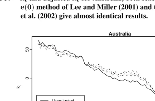
The three factors (fitting period, method of adjustment and jump-off rates) are inde-pendent for LC and LM. For BMS, choice of fitting period is deinde-pendent on the shape of the fittedkt, which in turn is influenced to some extent by the method of adjustment, particularly where deviations from linearity occur (see Figure 3).
Figure 3: ktand adjustedktfor Australia, both sexes combined, 1921–2000. The
e(0)method of Lee and Miller (2001) and theDx,tmethod of Booth et al. (2002) give almost identical results.
Australia
Year kt
1920 1940 1960 1980 2000
−100
−50
0
50
Unadjusted Dt adjustment e(0) adjustment Dxt adjustment
The mean absolute error in log death rates from each of the combinations is given in Table 6, averaged over country, sex, forecast year and age. The mean absolute error in life expectancy is similarly given in Table 7. In both tables, the LC, LM and BMS variants are marked in bold.
Table 6: Mean absolute error in log death rates for different Lee-Carter variations, averaged over country, sex, forecast year and age. The LC, LM and BMS variants are marked in bold.
Jump-off: Fitted Actual
Adjustment: None Dt e(0) Dx,t None Dt e(0) Dx,t Fitting period
long 0.236 0.384 0.309 0.300 0.177 0.184 0.181 0.181
1950 0.175 0.187 0.179 0.178 0.171 0.171 0.171 0.171
Table 7: Mean absolute error in life expectancy for different Lee-Carter variations, averaged over country, sex and forecast year. The LC, LM and BMS variants are marked in bold.
Jump-off: Fitted Actual
Adjustment: None Dt e(0) Dx,t None Dt e(0) Dx,t Fitting period
long 1.809 0.775 0.802 0.983 0.826 0.718 0.744 0.764
1950 0.956 0.850 0.758 0.878 0.749 0.756 0.735 0.757
short 0.492 0.535 0.498 0.534 0.484 0.498 0.494 0.502
The effect of different fitting periods is essentially measuring the effect of different trends inkt. It is seen that mean absolute error in log death rates is consistently greatest for the long fitting period, while mean error in life expectancy is consistently smallest for the short fitting period. The use of 1950 to define the fitting period produces less consistent results: for log death rates some errors are smallest while for life expectancy some errors are largest. These results refer, of course, to the 15-year forecasting period under consideration; a different pattern may emerge for longer forecasting periods.
The effect of adjustment is small compared with the effect of fitting period and jump-off bias, and in some cases is extremely marginal. When fitted jump-jump-off rates are used, any adjustment worsens the forecasts of log death rates; this is partly because the fit to the base model is no longer statistically optimal. Adjustment toDtconsistently produces the largest errors in log death rates. For life expectancy, any adjustment tends to improve the forecast, except with a short fitting period, but the optimal adjustment varies. The effect of the different adjustments on life expectancy is complex and depends on the cancellation of errors.
Comparison of fitted and actual jump-off rates gives an indication of the contribution of jump-off error to forecast error. Using actual jump-off rates is generally advantageous. The gain in accuracy is largest when the fitting period is long and when adjustment toDt is used. This explains why jump-off error is particularly large for LC (as indicated by Figures 1 and 2). When forecast error is small, jump-off error is marginal. When actual rates are used there are only marginal differences in errors in log death rates between fitting periods or adjustment methods. Given the potentially significant error associated with the use of fitted jump-off rates, actual jump-off rates would seem preferable.
Tables 6 and 7 show that amongst the three variants, BMS is best for both accuracy measures (log death rates and life expectancy). However, the tables suggest that a better method would use the short fitting period of BMS, but with no adjustment. In fact, for log death rates, the use of no adjustment is most accurate in all cases.
of life expectancy rates is from 0.775 to 0.484 or 38%, but poorer accuracy also occurs (despite not occurring for log death rates).
By way of comparison, the mean absolute error in log death rates for HU is 0.149 and for DJT is 0.150 (an improvement of 61% over LC in both cases). The mean absolute error in life expectancy for HU is 0.657 and for DJT it is 0.711. This is consistent with the earlier findings, that HU and DJT are more accurate than the other methods in fore-casting log death rates, but this doesn’t translate into greater accuracy for life expectancy forecasts. An indication of the gain in accuracy attributable to the greater statistical so-phistication of HU and DJT can be obtained by comparing them with the four results for 1950/fitted rates. The maximum gain in accuracy for HU is 20% for log death rates and 31% for life expectancy. DJT achieves gains of up to 20% and 26% respectively.
6. Discussion and conclusions
The results of this comparative evaluation of forecasts for the period 1986–2000 show that while each of the four variants and extensions is more accurate in forecasting log death rates than the original Lee-Carter method, none is consistently more accurate than the others. It was found that on average HU and DJT provided the most accurate forecasts of log death rates; however, the differences among the four methods are small and are not significant. BMS provided marginally more accurate forecasts of life expectancy but there were no significant differences between the five methods for this measure.
The changed ranking of methods depending on the measure of interest highlights the conceptual problem in defining forecast accuracy. Demographers have traditionally fo-cussed on life expectancy but, as has been seen, there is little relation between the relative accuracy of this measure and that of the underlying log death rates which are actually modelled. The two transformations, namely exponentiation and the life table (involving the cancellation of errors and implicit weights), are highly complex in combination such that the finer degree of accuracy in forecasting life expectancy is largely a matter of luck. Even if forecast life expectancy is accurate, compensating age-specific errors can be rel-atively substantial (see Figure 1) and in the long-term lead to unrealistic forecasts of the age pattern of mortality, with flow-on effects on forecasts of population structure. While accuracy in forecasting life expectancy may be important, it is not sufficient. To gain an understanding of forecast error, the evaluation of error in log death rates is essential.
when the model is not a good fit to the data. However, there is no compelling evidence in favour of any of the adjustment methods. Further, among the possible combinations of factors, the combination of short fitting period, no adjustment ofktand fitted jump-off rates produced the smallest errors in log death rates (0.154) while actual jump-off rates were more advantageous for life expectancy. Either of these combinations might thus be adopted at least for the short forecast horizons considered here.
There is some evidence that the absolute error in the log death rates increases as the fitting period increases in length. This suggests that model misspecification may be present, probably due to the assumed linearity in modellingktand the assumed fixed age pattern of change,bx. Given a changing pattern of mortality decline, such as occurred over the twentieth century, a shorter fitting period often results in more appropriatektand bxfor the forecasting period. This highlights the limitations of the model for longer fitting periods. The random walk with drift model is in general a poor model forktbecause it does not allow for dynamic changes in slope. Shorter fitting periods tend to work better with this model (at least for shorter forecast horizons) because they capture the most recent trend. Adaptive time series models such as those inherent in HU and DJT, which place more weight on recent than distant experience, tend to perform better for the same reason; our empirical results support this for the fifteen-year period in question. Similarly, the assumption of fixedbx is less of a limitation for shorter fitting periods because the recent pattern of change is most relevant. HU overcomes this assumption to some extent by the use of multiple functions, thus allowing for more flexible mortality changes.
It is noted that Tuljapurkar et al. (2000) did not adjustkt; they combined this with the 1950 fitting period and fitted jump-off rates. The results of this evaluation show that, for 1950/fitted rates, the choice of no adjustment is advantageous for the accuracy of forecast log death rates but disadvantageous for the accuracy of life expectancy. While these effects are moderate for the 1950 fitting period, they are substantial when the long fitting period is used. It is seen in Figure 3 that adjustment makes a noticeable difference to the trend inkt: specifically, when no adjustment is used the decline is less rapid leading to a lower fitted life expectancy in the jump-off year. This general pattern is observed for all ten populations included in this evaluation. (When the fitting period begins in 1950, adjustment makes little difference to the trend.) For life expectancy, the slower rate of increase from a lower jump-off point produces significant underestimation especially in the longer term. Thus caution should be exercised in using no adjustment with longer fitting periods, especially when combined with fitted jump-off rates.
dominate total error (Figure 2). The indication that actual jump-off rates give greater fore-cast accuracy than fitted rates might be regarded as undermining the model. However, in all three Lee-Carter variants the model is already less than statistically optimal by virtue of the adjustment ofkt. BMS and HU aim to reduce jump-off bias by achieving a better fit to the underlying model; for HU this also involves the use of several basis functions. It is noted that the drift term of a random walk with drift is defined by the first and last points of the fitting period. Thus the better the fit of the underlying model (or its first basis function) to the last point in particular, the smaller the jump-off bias and the more accurate the drift.
The LM variant is, in fact, widely referred to by Lee and others as the Lee-Carter method and it is this variant that is now widely applied. However, the original Lee-Carter method (specifically adjustment ofktto match total deaths) is still used as a point of reference (e.g. Renshaw and Haberman, 2003c; Brouhns et al., 2002). This analysis suggests that not only is the original LC method a rather poor point of reference when the evaluation is focused on log death rates, but also that the LM variant is not the optimal point of reference (at least on the basis of these averaged results). Actual jump-off rates and no adjustment ofktappears to be a better point of reference for all but the short fitting period where fitted rates are advantageous. Bongaarts (2005) uses as a reference the Lee-Carter method without adjustment. Actual rates may be replaced by the average observed rates over the last two or three years of the fitting period (Renshaw and Haberman, 2003a).
There has been no attempt in this paper to compare the five forecasting methods on any basis other than forecast accuracy. Further research is needed to compare forecast uncertainty among the five methods; a comparison of LC and BMS standard errors and prediction intervals appears in Booth et al. (2002). HU and DJT provide a general frame-work that is readily adapted to deal with more complex forecasting problems including forecasting several populations with related dynamics such as a common trend. They also produce forecast rates that are smooth across age, which may be an advantage in some applications.
and the countries included, however, these methods do not deliver a marked increase in forecast accuracy.
A final consideration is the ease with which the methods can be implemented. To this end, Hyndman (2006) is an R package which implements the HU, LC, LM and BMS methods, as well as other variants of the Lee-Carter method.
7. Acknowledgments
References
Bell W R. (1997). “Comparing and assessing time series methods for forecasting age-specific fertility and mortality rates.”Journal of Official Statistics, 13 (3): 279–303.
Bell W R, Monsell B. (1991), “Using principal components in time series modelling and forecasting of age-specific mortality rates.” In: Proceedings of the American Statistical Association, Social Statistics Section, 154–159.
Bongaarts J. (2005). “Long-range trends in adult mortality: Models and projection meth-ods.”Demography, 42 (1): 23–49.
Booth H. (2006). “Demographic forecasting: 1980 to 2005 in review.”International Jour-nal of Forecasting, 22 (3), 547–581.
Booth H, Maindonald J, Smith L. (2002). “Applying Lee-Carter under conditions of vari-able mortality decline.”Population Studies, 56 (3): 325–336.
Booth H, Tickle L, Smith L. (2005). “Evaluation of the variants of the Lee-Carter method of forecasting mortality: a multi-country comparison.”New Zealand Population Re-view, 31 (1): 13–34.
Brouhns N, Denuit M, Vermunt J K. (2002). “A Poisson log-bilinear regression approach to the construction of projected lifetables.”Insurance: Mathematics and Economics, 31 (3): 373–393.
Buettner T, Zlotnik H. (2005). “Prospects for increasing longevity as assessed by the United Nations.”Genus, LXI (1): 213–233.
Currie I D, Durban M, Eilers P H C. (2004). “Smoothing and forecasting mortality rates.”
Statistical Modelling, 4 (4): 279–298.
De Jong P, Tickle L. (2006). “Extending Lee-Carter mortality forecasting.”Mathematical Population Studies, 13 (1): 1–18.
Girosi F, King G. (2006), Demographic forecasting. Cambridge: Cambridge University Press.
Harvey A C. (1989), Forecasting, structural time series models and the Kalman filter. Cambridge: Cambridge University Press.
Hastie T, Tibshirani R. (1990), Generalized additive models. London: Chapman & Hall/CRC.
Hyndman R J, ed. (2006), demography: Forecasting mortality and fertility data. URL http://www.robhyndman.info/Rlibrary/demography, R package.
Hyndman R J, Koehler A B, Snyder R D, Grose S. (2002). “A state space framework for automatic forecasting using exponential smoothing methods.”International Journal of Forecasting, 18 (3): 439–454.
Hyndman R J, Ullah M S. (2007). “Robust forecasting of mortality and fertility rates: a functional data approach.”Computational Statistics and Data Analysis, to appear.
Keyfitz N. (1991). “Experiments in the projection of mortality.”Canadian Studies in Pop-ulation, 18 (2): 1–17.
Lee R D, Carter L R. (1992). “Modeling and forecasting U.S. mortality.”Journal of the American Statistical Association, 87: 659–675.
Lee R D, Miller T. (2001). “Evaluating the performance of the Lee-Carter method for forecasting mortality.”Demography, 38 (4): 537–549.
Lee R D, Tuljapurkar S. (1994). “Stochastic population forecasts for the United States: beyond high, medium, and low.”Journal of the American Statistical Association, 89: 1175–1189.
Li N, Lee R D, Tuljapurkar S. (2004). “Using the Lee-Carter method to forecast mortality for populations with limited data.”International Statistical Review,72, 1: 19–36.
Lundström H, Qvist J. (2004). “Mortality forecasting and trend shifts: an application of the Lee–Carter model to Swedish mortality data.”International Statistical Review, 72 (1): 37–50.
Lutz W, Goldstein J., ed. (2004), How to deal with uncertainty in population forecasting? IIASA Reprint Research Report RR-04-009. Reprinted fromInternational Statisti-cal Review, 72 (1&2): 1–106, 157–208.
Makridakis S G, Wheelwright S C, Hyndman R J. (1998), “Forecasting: methods and applications.” New York: John Wiley & Sons, 3rd edition.
Murphy M J. (1995). “The prospect of mortality: England and Wales and the United States of America, 1962–1989.”British Actuarial Journal, 1 (2): 331–350.
Ramsay J O, Silverman B W. (2005), “Functional data analysis.” New York: Springer-Verlag, 2nd edition.
Renshaw A E, Haberman S. (2003a). “Lee-Carter mortality forecasting: a parallel gen-eralized linear modelling approach for England and Wales mortality projections.”
Renshaw A E, Haberman S. (2003b). “Lee-Carter mortality forecasting with age-specific enhancement.”Insurance: Mathematics and Economics, 33 (2): 255–272.
Renshaw A E, Haberman S. (2003c). “On the forecasting of mortality reduction factors.”
Insurance: Mathematics and Economics, 32 (3): 379–401.
Trefethen L N, Bau D. (1997), “Numerical linear algebra.” Philadelphia: Society for In-dustrial and Applied Mathematics.
Tuljapurkar S, Li N, Boe C. (2000). “A universal pattern of mortality decline in the G7 countries.”Nature, 405: 789–792.
Wilmoth J R. (1996), “Mortality projections for Japan: a comparison of four methods.” In: Caselli G, Lopez A, editors. Health and mortality among elderly populations. New York: Oxford University Press: 266–287.