Exact Solutions of two-Dimensional Nonlinear Schrödinger Equations with External Potentials

Published online December 30, 2013 (http://www.sciencepublishinggroup.com/j/acm) doi: 10.11648/j.acm.20130206.18

Exact solutions of two-dimensional nonlinear Schrödinger

equations with external potentials

Nalan Antar

1, *

, Nevin Pamuk

2

1

Department of Mathematics, Istanbul Technical University, Maslak 34469, Istanbul, Turkey

2

University of Kocaeli, Kocaeli Vocational High School, Kullar, 41300, Kocaeli – TURKEY

Email address:

[email protected] (N. Antar)

To cite this article:

Nalan Antar, Nevin Pamuk. Exact Solutions of two-Dimensional Nonlinear Schrödinger Equations with External Potentials. Applied and Computational Mathematics. Vol. 2, No. 6, 2013, pp. 152-158. doi: 10.11648/j.acm.20130206.18

Abstract:

In this paper, exact solutions of two-dimensional nonlinear Schrödinger equation with kerr, saturable and quintic type of nonlinearities are studied by means of the Homotopy analysis method (HAM). Linear stability properties of these solutions are investigated by the linearized eigenvalue problem. We also investigate nonlinear stability properties of the exact solutions obtained by HAM by direct simulations.

Keywords:

Homotopy Analysis Method, Nonlinear Schrödinger Equation, Stability

1. Introduction

In recent years, there have been so many mathematical methods to find approximate solutions of non-linear problems which come from various field of science and engineering [1]-[5] [6]-[14]. One of them is Homotopy analysis method (HAM). Homotopy analysis method, originally presented by Liao in 1992, has embedding parameters p and non-zero auxiliary parameter h which provides us with a simple way to adjust and control the radius of convergence of series solution. Later, this parameter h is called convergence-control parameter.

Solitons are localized nonlinear waves and occur in many branches of physics. Their properties have provided fundamental understanding of complex nonlinear systems. In recent years there has been considerable interest in studying solitons in system with periodic potentials or lattices, in particular, those that can be generated in nonlinear optical materials ([15]-[18]) in order to get stable solitons. In two-dimensional geometry, fundamental solitons are unstable in two-dimensional NLS equation with cubic nonlinearity. The Optical lattices such as periodic and quasicrystal lattices, are not necessary for stability of the solitons in the self-focusing cubic media [19].

The purpose of the paper, we obtain explicit series solutions of nonlinear Schrödinger equations with an external potential under kerr, saturable and quintic nonlinearities by Homotopy analysis method. The nonlinear stability of the exact solutions of NLS equation with kerr,

cubic and saturable nonlinearities under the external potential are studied by direct computations. We also investigate the linear spectrum of the exact solutions by using the Fourier Collocation method ([20]).

2. Homotopy Analysis Method

In this section, we apply the homotopy analysis method to two-dimensional nonlinear Schrödinger equation with kerr, saturable and quintic nonlinearities under the external potentials.

In order ro show the basic idea of HAM, let us consider the following nonlinear differential equation

0

=

)]

,

(

[

u

r

t

N

(1)

where N is a nonlinear operator that represents the whole equation,

r

and

t

are independent variables and u(r,t) is an unknown function respectively. By means of generalizing the traditional homotopy, Liao constructs a new homotopy which is called zero-order deformation equation ([1],[10], [11]). This homotopic equation is the following

),

(

)

,

(

=

)]

(

)

(

)[

approximate function and Φ(r,t;p) is an unknown function. Obviously, when p=0 and p=1, it holds

)

,

(

=

;0)

,

(

r

t

u

₀

r

t

Φ

(3)

)

,

(

=

;1)

,

(

r

t

u

r

t

Φ

(4)

respectively. So, as

p

increases from 0 to 1, Φ(r,t;p) varies from the initial guess

u

₀ to

u

.

Expanding

) ; , (rt p

Φ in Taylor series with respect to the

p

, we can write

... ) , ( ) , ( ) , ( = ) ; ,

( ₀ + ₁ + 2 ₂ +

Φr t p u rt pu r t p u r t (5) where

.

|

!

1

=

)

,

(

_p=0

k k

k

p

k

t

r

u

∂

Φ

∂

(6)

If the auxiliary linear operator, the initial guess, the convergence control parameter

h

, and the auxiliary function are properly chosen, then the above series converges at p=1, which is proved by [1]. So we can find infinite series as

.... ) , ( ) , ( ) , ( = ) ; , ( lim = ) ,

( _{0 1 2}

1

+ +

+ Φ

→ rt p u rt u r t u r t

t r u

p (7)

3. The Exact Solution of NLS Equation

with an External Potential

In this study, we investigate the exact solutions of two-dimensional NLS equation with external potentials by using the HAM method. The generalized NLS equation we consider is

0. = ) , | (|u 2 u F u

iut+∆ + (8)

Here F(? is a real function, and we assume 0

= (0)

F .This equation describes nonlinear light propagation in a non-Kerr medium. u x y t( , , ) corresponds to the complex-valued, slowly varying amplitude in the

xy

plane propagating in the

t

direction, ∆u≡uxx +uyy

corresponds to diffraction. In this paper, F(|u|2,u)

function will be taken in the following form:

(a)If we take F(|u|2,u)=|u|2u+V_d(x,y)u the Nonlinear Schrödinger equation describe soliton propagating along the t direction in optical medium with spatially Kerr-type nonlinearity.

(b) If we take F(|u|2,u)=|u|4u+V_d(x,y)u, the quintic nonlinear Schrödinger (QNLS)equation is obtained and

) , (x y

V_d is an external potential .

(c) If 2 2

0

(| | , ) = / (1 d( , ) | | ) F u u E u +V x y + u the governing equation is NLS equation with saturable nonlinearity. Here E₀ is a constant. V_d(x,y) is the external potential.

We will give the exact solutions of Nonlinear Schrödinger equation with external potentials under the kerr, saturable and quintic nonlinearities respectively.

3.1. Nonlinear Schrödinger Equation with Kerr type Nonlinearity

We analyze two-dimensional nonlinear Schrödinger equation based on a type of non periodic modulation of linear refractive index in the transverse direction. We obtain an exact solution in explicit form for (2 + 1)D nonlinear Schrödinger equation with the non periodic modulation [5].

0

=

|

|

)

,

(

)

(

2

1

2

u

u

u

y

x

V

u

u

iu

_t

+

_xx

+

_yy

+

_d

+

(9)

with the initial condition

)].

(

2

[

exp

=

,0)

,

(

x

y

k

x

2

y

2

u

ξ

−

+

(10)

We consider the non periodic modulation of the linear refractive index in the transverse direction under a parabolic and Gaussian distribution, i.e.,

)] (

[ exp ) (

2 = ) ,

(x y k x2 y2 k x2 y2

V_d − + −ξ − + (11)

We apply HAM to the Eq.(9) with initial condition

)] (

2 [ exp = ,0) ,

(x y k x2 y2

u ξ − + In order to solve Eq.(9),

we construct the homotopic equation. If we substitute 1

= ) , (rt

H into Eq.(2), then we obtain

)] ( [ = )] ( ) ( )[

(1−p LΦ −Lu_o phN Φ (12)

where

t L

∂ Φ ∂ Φ)=

( and

N

is the whole operator

Φ Φ + Φ +

Φ + Φ + Φ

Φ 2

| | ) , ( ) (

2 1 = )

( i V x y

N t xx yy d and

u

0

is the zeroth order approximate function which we take

)] (

2 [ exp = ,0) , (

= 2 2

0 x y

k y

x u

u ξ − + . If we substitute L,

N ,and

u

₀ into the Eq.(12), then homotopic equation becomes

2

( 1 ) ( )

= 2

( , ) | |

t x x y y

t

d

h i h

i p

h V x y h

+ Φ + Φ + Φ +

Φ

Φ + Φ Φ

 

 

 

 

(13)

)], ( 2 [ exp = ,0) , ( 0, = {

: 0 0 2 2

0 y x k y x u t u

p − +

∂

∂ _ξ

2 2

1 1 0 0 0

2 2

2

0 0 0

: = ( 1) 2 ( , ) | | ,

d

u u u

u h

p i h

t t x y

hV x y u h u u

∂ _{∂ ∂}  ∂ _{+ + + +}   ∂ ∂  ∂ ∂  + 2 2

2 2 1 1 1

1

2 2

2 2

0 1 1

: = ( 1) ( , )

2

(2 | | ),

d

o

u u h u u

p i h hV x y u

t t x y

h u u u u

  ∂ ₊ ∂ ₊ ∂ ₊∂   ∂ ∂ ∂ ∂  + + 2 2

3 3 2 2 2

2

2 2

2 2 2 2

0 2 1 0 1 0 0 2

: = ( 1) ( , )

2

(2 | | 2 | | ),

d

u u h u u

p i h hV x y u

t t x y

h u u u u u u u u

∂ _∂ _{∂ ∂} 

+ +  + +

∂ ∂  ∂ ∂ 

+ + + +

⋮

with the initial conditions u₁=u₂ =u₃=...=0. If we solve above equations for unknowns

u

_i

'

s

, we obtain

)], (

2 [ exp

= 2 2

0 x y

k

u ξ − +

)] (

2 [ exp

= 2 2

1 x y

k ihkt

u ξ − +

)], ( 2 [ exp ) 2 (

= 2 2

2

2 x y

k t hik t ht ihk

u ξ + + − +

3

2 2 2 2

3

2 2

= ( 1) ( 1)

6

exp[ ( )]

2

t

u hk i h t hk h t h k i x

k

x y

ξ + − + − 

 

− ₊

⋮

As a result, if we sum up the terms u_i's for h=−1 and 1

=

p , we can get the solution in Taylor from as

2

2 2

( )

( , ) = 1 ... exp[ ( )]

1! 2! 2

ikt ikt k

u x t ξ +− + − +  − x +y

  (14)

The closed-form solution is

). ( exp )] ( 2 [ exp = ) ,

(x t k x2 y2 ikt

u

ξ

− + − (15)

3.2. Saturable-Nonlinear Schrödinger Equation

The propagation of a polarized probe beam is governed by a generalized NLS equation with saturable nonlinearity. The model can be given as follows

0 = | | ) , ( 1 2 0 u y x V u E u u iu d yy xx t + + − +

+ (16)

with the initial condition ( )] 2 [ exp = ,0) ,

(x y k x2 y2

u ξ − + .

Where (x,y) are transverse coordinates, u is the slowly-varying amplitude of the probe beam, E0 is a

constant and V_d is a lattice intensity function as following

)]. ( [ exp ) ( ) ( = ) ,

( 2 2

2 2 2 2 2 2

0 _{k x y}

y x k y x k E y x

V_d − − +

+ +

− _ξ

(17)

we apply HAM to the Eq.(16) with initial condition

)] ( 2 [ exp = ,0) ,

(x y k x2 y2

u ξ − + . In order to solve Eq.(16),

we construct the homotopic equation. If we substitute

1 = ) , (rt

H into Eq.(2), then we obtain

)] ( [ = )] ( ) ( )[

(1−p LΦ −Lu_o phN Φ (18)

where t L ∂ Φ ∂ Φ)=

( and N is the whole operator

) ( | | ) , ( 1 = )

( 0 _{2 xx yy}

d t y x V E i

N − Φ +Φ

Φ + + Φ + Φ Φ

and

u

₀ is the zeroth order approximate function. If we

substitute

_L

, N,and

u

₀ into the Eq.(12), then homotopic equation becomes         Φ + Φ − Φ + + Φ + Φ +

Φ ( )

| | 1 1) (

= 0 ₂ xx yy

d t t V E h i p

i (19)

Substituting Eq.(5) into Eq.(19) and equating coefficients of

p

, we obtain

)], ( 2 [ exp = ,0) , ( 0, = {

: 0 2 2

0 y x k y x u t u i

p − +

∂

∂ _ξ

2 2

1 1 0 0 0

2 2

0 0 2 0

: = ( 1)

, 1 _d( , ) | |

u u u

u

p i i h h

t t x y

E u h

V x y u

∂ _{∂ ∂}  ∂ _{+ + +}   ∂ ∂ ∂ ∂  − + + 2 2

2 2 1 1 1

2 2

0 1 0 0 1 0 0 1

2

0 0 0 0

: = ( 1)

( )

,

1 _d (1 _d )

u u u u

p i i h h

t t x y

E u h E u h u u u u

V u u V u u

2 2

3 3 2 2 2

2 2

2 2 2

0 2 0 0 1 1 1 0 0 2 0 2

2

0 0 0 0

2 0 0 1 0 0 1

3 0 0

: = ( 1)

(2 )

(1 ) (1 )

( )

,

(1 )

d d

d

u u u u

p i i h h

t t x y

E u h E h u u u u u u u u u

V u u V u u

E u h u u u u V u u

∂ ∂ ∂ ∂  + +  +  ∂ ∂  ∂ ∂  + + + − + + + + + + + +

⋮

with the initial conditions u₁=u₂ =u₃=...=0. If we solve above equations for unknowns

u

_i

'

s

, we obtain the following functions

2 2 0

2 2 1

2 2 2 2 2

2

3 3 3

2 2 2 2

3

2 2

( , , ) = exp[ ( )], 2

= 2 exp[ ( )] 2

= 2[ ( 1) ] exp[ ( )], 2

4

= [ 4 ( 1) 2 ( 1) ] 3

exp[ ( )] 2

k

u x y t x y

k

u hkit x y

k

u h k t hk h it x y

ih k t

u h k t h ihkt h

k x y ξ ξ ξ ξ − ₊ − ₊ − − + + + − _{− + + +} − ₊ ⋮ (20)

As a result, if we sum up the terms u_i's for

_h

₌

−

₁

and p=1, we obtain the exact solution of the nonlinear Schrödinger equation under the saturable nonlinearity with an external potential as

)] ( 2 [ exp ... 3! ) (2 2! ) (2 1! 2 1 = ... ) , ( ) , ( ) , ( = ) ,

( 2 2

3 2

2 1

0 x y

k ikt ikt ikt t x u t x u t x u t x

u − +

        + − + − + +

+ ξ (21)

2 2

( , ) = exp[ ( 4 )]. 2

k

u x t ξ − x +y + it (22)

3.3. The Quintic-Nonlinear Schrödinger Equation

We obtain the exact solution of the nonlinear Schrödinger equation with quintic nonlinearity. The mathematical model can be given as

0 = | | ) , ( ) ( 2 1 4 u u u y x V u u

u_t+ _xx + _yy + _d + (23)

with the initial condition

)]. ( 2 [ exp = ,0) ,

(x y k x2 y2

u − + (24)

We consider the external potential as the non periodic modulation of the linear refractive index in the transverse direction which is a parabolic and Gaussian distribution, i.e.,

)] ( 2 [ exp ) ( 2 = ) ,

( 2 2 2 2

2 y x k y x k y x

V_d − + − − + (25)

We apply HAM to the Eq.(23) with initial condition

)] ( 2 [ exp = ,0) ,

(x y k x2 y2

u − + In order to solve Eq.(23), we

construct the homotopic equation. If we substitute 1

= ) , (rt

H into Eq.(2), then we obtain

)] ( [ = )] ( ) ( )[

(1−p LΦ −Lu_o phN Φ (26)

where t L ∂ Φ ∂ Φ)=

( and N is the whole operator

Φ Φ + Φ + Φ + Φ + Φ Φ 4 | | ) , ( ) ( 2 1 = )

( i V x y

N t xx yy d

and is the zeroth order approximate function which we take

)] (

2 [ exp

= 2 2

0 x y

k

u − + . If we substitute L,

N

,and

u

₀

into the Eq.(12), then homotopic equation becomes

      Φ Φ + Φ + Φ + Φ + Φ +

Φ _{( ) ( , ) | |}4

2 1) (

=pih h hV x y h

i _{t t xx yy d} (27)

Substituting Eq.(5) into Eq.(27) and equating coefficients of

p

, we obtain

)], ( 2 [ exp = ,0) , ( 0, = {

: 0 2 2

0 y x k y x u t u

p − +

∂ ∂

2 2

1 1 0 0 0

2 2

4

0 0 0

: = ( 1) 2

( , ) | | ,

d

u u u

u h

p i h

t t x y

hV x y u h u u

∂ ∂ ∂  ∂ _{+ + +}   ∂ ∂  ∂ ∂  + + 2 2

2 2 1 1 1

2 2

2 2 3

1 0 1 0 0 1 0

: = ( 1) 2

( , ) (3 2 ),

d

u u h u u

p i h

t t x y

hV x y u h u u u u u u

  ∂ ₊ ∂ ₊ ∂ ₊∂   ∂ ∂ ∂ ∂  + + + 2 2

3 3 2 2 2

2 2

2 2 2

2 0 0 1 1 0 1 0

2 2 2 3 3

0 2 0 1 0 2 0 0

: = ( 1)

2

( , ) (6 3

3 2 ),

d

u u h u u

p i h

t t x y

hV x y u h u u u u u u u u u u u u u u u

∂ _∂ _{∂ ∂}  + +  +  ∂ ∂  ∂ ∂  + + + + + +

⋮

with the initial conditions u₁=u₂=u₃=...=0. If we solve above equations for unknowns

u

_i

'

s

, we obtain

)], (

2 [ exp

= 2 2

0 x y

k

)] (

2 [ exp

= 2 2

1 x y

k ihkt

u − +

)], (

2 [ exp 1)] ( 2

[

= 2 2

2 2 2

2 x y

k h

hkit t k h

u − + + − +

3 3 3

2 2 2 3

2 2 2

= [ ( 1 )

6

( 1 ) ] e x p [ ( ) ] ,

2 i h k t

u h k t h

k

h k i t h x y

− _{− +}

−

+ + +

⋮

With the same manipulating as we did above examples, summing up the termsq u_i's for h=−1 and

p

=

1

, we obtain the exact solution of the Nonlinear Schrödinger equation in the following form

2 2

( , ) = exp[ ( 2 )]. 2

k

u x t − x +y + ikt (28)

4. Linear and Nonlinear Stability of the

Exact Solutions

4.1. Linear Stability

Now we address the critical question of linear stability of these exact solution under kerr, saturable and quintic nonlinearities. To obtain the whole spectrum of these solutions, we will use the Fourier collocation method ([20]). We consider NLS equation with general types of nonlinearities and potentials

0 = ] , | [|U 2 x F U

iU_t+∆ + (29) Here F(|U|2,x) is a real-valued function. This equation admits solutions of the form

t i e x u t x

U( , )= ( ) µ (30) where

µ

is the propagation constant, and

u

(x

)

is a general real-valued function. To study the spectrum of the exact solutions we assume that [20]

t i t t

e e x w x v e x w x v x u t x

U( , )=[ ( )+[ ( )+ ( )] λ +[ *( )− *( )] λ*] µ (31)

where v(x),w(x)<<1 . Inserting this solution given in Eq.( 24) to Eq. (22) and linearizing, we obtain the following linear-stability eigenvalue problem as

  

 

  

 

  

 

  

 

  

 

  

 

+ −

w v w v L

L

λ

= 0 0

i (32)

where

L

₋ and

L

₊ are defined as

2 2 2

2

| | 2 ) , | (| =

) , | (| =

u F u x u F L

x u F L

∂ ∂ + +

∆ + −

+ ∆ + −

+ −

µ µ

(33)

Eigenvalues with positive real parts are unstable eigenvalues. The other eigenvalues are stable ( purely imaginary eigenvalues are often called internal modes). We checked the linear eigenvalue problem for these exact solutions obtained by the use of the homotopy analysis method.

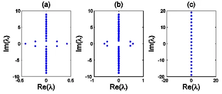
The linear spectrum of the exact solutions of nonlinear Shcrödinger equation for kerr and quintic nonlinearity under the parabolic and gaussian distribution are shown in Fig. 1.

Figure 1. Linear-stability spectra of the exact solutions (15) (28) and (22) (with k= -1) in the generalized NLS equation under three different nonlinearities (a) Kerr nonlinearity (b) Quintic nonlinearity (c) Saturable nonlinearity.

As it seen from this figure the spectrum of the exact solutions of NLS equation with kerr and quintic nonlinearity contains a pair of real eigenvalues. So these solutions are linearly unstable while the exact solution of NLS equation for saturable nonlinearity under the parabolic and gaussian distribution is linearly stable.

4.2. Nonlinear Stability

In order to study the nonlinear stability, we directly compute the (2+1) dimensional NLS equation with kerr, quintic and saturable nonlinearities over a long time, (finite difference method was used on derivatives

u

_xx and

u

_yy, and fourth-order Runge-Kutta method to advance in t) for periodic and gaussian distribution potentials. The initial conditions were taken to be an exact solutions with

%1

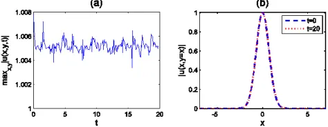
random noise in the amplitude and phase. First we consider the direct simulations of the exact solution of NLS equation with kerr nonlinearity. As can be seen from Figure. 2 the peak amplitude of the exact solution A t( ) =maxx y, | |u

Figure 2. (a) Peak amplitude A t( ) =maxx y_, | |u of the exact solution of NLS equation with kerr nonlinearity as a function of the propagation time. The initial condition is taken as the exact solution with 0.01 noise. in the amplitude and phase. (b) On the axis mode profile for exact solution for kerr nonlinearity along the diagonal axes with t=0 and t=20.

The second case we plotted the maximum amplitude of the exact solutions for quintic and saturable nonlinearity. Figure 3 and Figure 4 show that the maximum amplitude for both cases oscillate with

t

. The exact solutions appear to be nonlinearly stable.

Figure 3. (a) Peak amplitude A t( ) =maxx y_, | |u of the exact solution of

NLS equation with quintic nonlinearity as a function of the propagation time. The initial condition is taken as the exact solution with 0.01 noise in the amplitude and phase. (b) On the axis mode profile for exact solution for kerr nonlinearity along the diagonal axes with t=0 and t=20.

Figure 4. (a) Peak amplitude A t( ) =maxx y_, | |u of the exact solution of

NLS equation with saturable nonlinearity as a function of the propagation time. The initial condition is taken as the exact solution with 0.01 noise in the amplitude and phase. (b) On the axis mode profile for exact solution for kerr nonlinearity along the diagonal axes with t=0 and t=20

5. Conclusion

In this paper, using different types of nonlinearities, we found the exact solutions of two-dimensional nonlinear Shrödinger equation with the parabolic and gaussian distribution by using Homotopy analysis method (HAM ). We also investigate the nonlinear and linear stabilities of the exact solutions. We show that all exact solutions for kerr, quintic and saturable nonlinearities are nonlinearly stable

but for kerr and quintic nonlinearity the exact solutions are linearly unstable. Also we investigated the linear stability of the exact soliton for saturable nonlinearity. We found that this solution is linearly stable.

References

[1] S.J.Liao, The proposed homotopy analysis technique for the solution of nonlinear problems, Ph.D thesis, Shanghai Jiao tong University, (1992)

[2] J.H.He, Homotopy perturbation technique, Comput.Methods Appl. Mech.Engrg 178(1999) 257-262.

[3] J.H.He, Homotopy perturbation method. A new nonlinear analytical Technique, Appl.Math.Comp. 135(2003)73-79.

[4] N.Pamuk, Series Solution for Porous Medium Equation with a Source Term by Adomian’s Decomposition Method, Appl. Math.Comput.178(2006)480-485.

[5] Y.Wang, R.Hao, Exact spatial soliton solution for nonlinear Schrödinger equation with a type of transverse non periodic modulation, Optics Communications 282 (2009)3995-3998.

[6] S.Pamuk, N.Pamuk, He’s Homotopy Perturbation Method for continuous population models for single and interacting species, Comp. and Math. with applications 59(2010)612-621.

[7] J.H. He, Homotopy Perturbation Method for Solving Boundary Value Problems, Physics Letters A 350(2006) 87-88.

[8] J.H.He, Recent devolopment of the Homotopy perturbation method, Topological methods in nonlinear analysis, 31(2008)205-209.

[9] Abbasbandy S, The application of Homotopy analysis method to nonlinear equations arising in heat transfer, Physics lett.A,360(2006) 109-13.

[10] Liao SJ, On the Homotopy analysis method for nonlinear problems, Appl. math.comp., 147(2004)499-513.

[11] Liao SJ, Numerically solving nonlinear problems by

Homotopy analysis method, Comput.mech.,

20(1997)530-40.

[12] J.H.He, Comparison of Homotopy perturbation method and homotopy analysis method, Applied Math. and comp.,156(2004) 527-539.

[13] J.H.He, An elementary introduction to the homotopy perturbation method, Comp. and Math. with Appl., 57(2009)410-412.

[14] S.Liang, D.J.Jeffrey, Comparison of homotopy analysis method and homotopy perturbation method through an evaluation equation, Commn nonlinear sci. numer. simulat., 14(2009)4057-4064.

[15] D. N. Christodoulides, F. Lederer, and Y. Silberberg, Nature, 424, 817 (2003).

[16] A. A. Sukhorukov, Y.S. Kivshar, H. S. Eisenberg, and Y. Silberberg, IEEE J. Quant. Electronics, 39, 31 (2003).

[18] J. W. Fleischer, M. Segev, N. K. Efremidis, and D. N. Christodoulides, Nature, 422, 147 (2003).

[19] M.J. Ablowitz, N. Antar, I. Bakrta

s

, B. Ilan, Phys, Rev. A, 81, (2010) 033834.