Reliability simulation of water distribution systems – single and multiquality

Reliability simulation of water distribution systems – single

and multiquality

Avi Ostfeld

, Dimitri Kogan

, Uri Shamir

Faculty of Civil Engineering, Israel Institute of Technology, Technion, Haifa 32000, Israel b

Chip Express Ltd., Matam, Israel

Received 31 January 2001; received in revised form 4 July 2001; accepted 28 August 2001

Abstract

An application of stochastic simulation for the reliability analysis of single and multiquality water distribution systems (MWDS) is formulated and demonstrated. MWDS refers to systems in which waters of different qualities are taken from sources, possibly treated, mixed in the system, and supplied as a blend. The stochastic simulation framework was cast in a reliability analysis program (RAP), based on EPANET, and quantifying three reliability measures: the fraction of delivered volume (FDV), the fraction of delivered demand (FDD), and the fraction of delivered quality (FDQ). RAP is demonstrated on two example applications: a simple illustrative, and a more ‘‘real-life’’ complex one. The results quantify the reliability of the systems and provide lower bounds for the reliability measures adopted.Ó2002 Elsevier Science Ltd. All rights reserved.

Keywords:Analysis; EPANET; Multiquality; Networks; Reliability; Software; Water distribution systems

1. Introduction

A water distribution system is an interconnected collection of sources, pipes, and hydraulic control ele-ments (e.g. pumps, valves, regulators, tanks) delivering water to consumers in prescribed quantities and at de-sired pressures. Such systems are often described in terms of a graph, with links representing the pipes, and nodes representing connections between pipes, hydraulic control elements, consumers, and sources. The behavior of a water distribution system is governed by:

1. physical laws that describe the flow relationships in the pipes and hydraulic control elements,

2. consumer demand, and 3. system layout.

Reliability analysis of a water distribution system is concerned with measuring its ability to meet consumers’ demands in terms of quantity and quality, under normal and emergency conditions. The required water quanti-ties and qualiquanti-ties are defined in terms of the flows to be supplied within given ranges of pressures and

concen-trations (e.g. residual chlorine, salinity). As such, water distribution systems play a vital role in preserving and providing a desirable life quality to the public, of which the reliability of supply is a major component.

The question: ‘‘Is a system reliable?’’ is usually un-derstood and easy to answer, while the questions ‘‘Is it reliable enough?’’ or ‘‘What is its reliability level?’’ are not straightforward, as they require both the quantifi-cation and calculation of reliability measures.

Thus, traditionally, reliability is defined by heuristic guidelines, like ensuring two alternative paths to each consumer node from at least one source, or having all pipe diameters greater than a minimum prescribed va-lue. By using such guidelines it is implicitly assumed that reliability will be assured, but the level of reliability provided is not quantified or measured. As a result, only limited confidence can be placed on such rules, as reli-ability is not considered explicitly.

In recent years there has been a growing interest in simulation approaches (e.g. Bao & Mays, 1990; Wagner, Shamir, & Marks, 1988a; Wagner, Shamir, & Marks, 1988b), with more emphasis put on explicit incorpora-tion of reliability in the design and operaincorpora-tion phases (e.g. Ostfeld & Shamir, 1996).

The quality of the water supplied is a growing concern, and more frequently ‘‘water’’ is no longer

*

Corresponding author. Tel.: +972-4-829-2782; fax: +972-4-822-8898.

E-mail addresses: [email protected] (A. Ostfeld), [email protected] (D. Kogan), [email protected] (U. Shamir).

considered a single commodity; water distribution sys-tems are becoming multi-commodity syssys-tems. Waters of different qualities are taken from sources, possibly treated, mixed in the system, and supplied as a blend. Such systems are termed multiquality water distribution systems (MWDS), serving all three types of consumers: domestic, industrial, and agricultural.

The concept of MWDS has been historically con-cerned with agricultural usage (e.g. Liang & Nahaji, 1983; Sinai, Koch, & Farbman, 1985), primarily in arid regions (e.g. the Arava valley in southern Israel, Cohen, Shamir, & Sinai, 1999a; Cohen, Shamir, & Sinai, 1999b; Cohen, Shamir, & Sinai, 2000) where good water quality is limited. Sources with different qualities are used in a single distribution system, with blending at nodes, being the predominant mechanism for adjusting the quality of the water supplied to consumers’ needs.

The objective of this paper is to formulate and dem-onstrate a stochastic simulation model for analyzing the reliability of single and MWDS. The model is termed reliability analysis program (RAP) and is based on EPANET (Rossman, 1994) – an extended hydraulic multiquality simulation model, upon which a stochastic simulation framework was built for reliability analysis.

The remainder of this paper consists of a brief liter-ature review on reliability analysis of water distribution systems, a description of RAP, and two example applications; a simple illustrative, and a more complex one.

2. Literature review

Reliability assessment of water distribution systems can be classified in two main categories: topological, and hydraulic. Following is a brief review.

2.1. Topological reliability

Topological reliability refers to the probability that a given network is connected, given its components me-chanical reliabilities, i.e. the components probabilities to remain operational at any time.

Wagner et al. (1988a) used reachability and connec-tivity to assess the reliability of a water distribution system, where reachability is defined as the probability that a given demand node is connected to at least one source, and connectivity as the probability that all de-mand nodes are connected to at least one source. Shamsi (1990), and Quimpo and Shamsi (1991) used node pair reliability (NPR), where the NPR measure is defined as the probability that a specific source node is connected to a specific demand node.

Measures used within this category consider only the connectivity between nodes (as in transportation or telecommunication network reliability models), but do not take into account the level of service provided to the consumers during a failure. The existence of a path be-tween a source and a consumer node in a water distri-bution system, in a non-failure mode or once a failure has occurred does not guarantee a sufficient service. This is because of the new re-distribution of flow and pres-sures in the system once a failure has occurred, governed by a non-linear law between flow and head (i.e. the Hazen Williams equation).

2.2. Hydraulic reliability

Hydraulic reliability is the probability that a water distribution system can supply consumers demands over a specified time interval under specified conditions. As such, hydraulic reliability refers directly to the basic function of a water distribution system; conveyance of Nomenclature

Ad the actual flow (demand) supplied at a

consumer node

FDD the fraction of delivered demand

FDDj the fraction of delivered demand at nodej

FDQ the fraction of delivered quality

FDQj the fraction of delivered quality at nodej

FDV the fraction of delivered volume

FDVj the fraction of delivered volume at nodej

Imax the prespecified number of simulation

repetitions

LRB lower reliability bound

MTOR maximum time of repair (h)

MWDS multiquality water distribution systems

N number of simulation runs

NN number of consumer nodes

P the actual pressure at a node

Pmin a threshold minimum pressure level

(Pmin in RAP is 40 psi for all nodes)

RAP reliability analysis program

Rd the requested consumer demand at a node

ti;j the total duration at run i, at nodej, for

which the demand supplied is above the demand factor

tqi;j the total duration at run i, at nodej, for

which the concentration is below the threshold concentration factor

T duration of each run

Vi;j the fraction of volume supplied to

consumerj at runi

VT the total requested volume of supply of

desired water quantities at desired pressures to desired locations at desired times.

The straightforward way to evaluate the hydraulic reliability of a system is through stochastic simulation (e.g. Bao & Mays, 1990; Fujiwara & Ganesharajah, 1993; Su, Mays, Duan, & Lansey, 1987; Wagner et al., 1988b). A typical stochastic (Monte Carlo) simulation procedure involves: generation of random component failure events; simulation of the system performance; and accumulation of performance statistics, with which reliability measures are evaluated. The data collected depend on what reliability measures are adopted. Con-ceptually, any index can be calculated, as long as the appropriate data is available.

Other references reviewing methods for assessing the reliability of water distribution systems were published by the ASCE task committee on risk and reliability analysis of water distribution systems (Mays, 1989), and by Engelhardt, Skipworth, Savic, Saul, and Walters (2000).

3. The model

The previous section summarized two approaches for assessing the reliability of water distribution sys-tems. Of these, in the current approach, stochastic simulation was chosen for evaluating system reliability. The rationale for this was that calculating the reliability of a system involves stochastic events, which should be assessed by probabilistic methods. Probabilistic meth-ods implicitly or explicitly account for the likelihood and effects of each system component redundancy, and so can be used for comparison and ranking of alter-native system designs and operation on the basis of reliability. Furthermore, once an initial assessment of the reliability of a water distribution system has been performed analytically (i.e. using a ‘‘topological’’ method); and alternative improvement options pro-posed, a stochastic simulation of these options can be carried to gain a better understanding of how the proposed alternative system are likely to behave under real-life conditions.

Three basic steps were implemented:

1. the definition of reliability measures (‘‘single’’ and ‘‘multiquality’’) reflecting chosen aspects of shortfalls as they relate to the consumers,

2. inclusion of the stochastic nature of performance of each system component, and of the consumers de-mands, and

3. coupling the previous two steps into a single frame-work that generates random events, runs EPANET, and evaluates, as a result, the system reliability ac-cording to the measures adopted in (1).

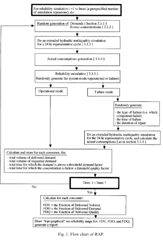
These were incorporated in RAP (described below, and in Fig. 1).

3.1. RAP

RAP involves running EPANET a prespecified number of times (i.e. a number high enough so that not to impact the final simulation outcomes. In the examples below 1000 times were usually satisfactory). For each run RAP repeats the following steps.

3.1.1. Random demand generation

Randomly generate, using a uniform probability distribution for each of the consumer nodes and within a given domain of fluctuations around average demand rates, the flow pattern to be used for the current run (i.e. average demands + ‘‘noise’’). Such a pattern repre-sents a typical demand cycle of 24 h (i.e. one realisa-tion of the demands at each of the nodes), as shown in Fig. 2.

3.1.2. Random source concentration generation

Randomly generate, using a uniform probability distribution within a given domain of concentration fluctuations around the average concentrations in the sources, the concentrations to be used at each of the sources for the current simulation run (i.e. average source concentrations + noise).

3.1.3. An extended hydraulic multiquality simulation

Carry out a multiquality simulation run with the flow pattern as in Section 3.1.1, and the concentrations at the sources as in Section 3.1.2.

3.1.4. Generation of actual consumptions

Estimate, according to the resulting pressures at the consumer nodes and an assumed relationship between the pressure at a consumer node and its corresponding flow rate (Wagner et al., 1988a), the actual flows sup-plied at the consumer nodes:

Ad ¼

Rd if PPPmin;

Rd

ffiffiffiffiffiffiffiffi Pmin

p pffiffiffiP if P<Pmin;

8 <

: ð1Þ

where Ad is the actual flow (demand) supplied at a

consumer node;Rdis the requested consumer demand at

a node; P is the actual pressure at a node; Pmin is a

threshold minimum pressure level (Pminin RAP is 40 psi

(26.7 m) for all nodes).

3.1.5. Reliability calculation

The system can be in either operational or failure mode. The system is said to be in a ‘‘failure mode’’ if one of its components (pipes, pumps, or sources) is out of service.

If the system is in anoperational mode, using the in-formation of steps 3.1.3 and 3.1.4, the following data are calculated and stored for each of the consumers: 1. The total volume of the delivered demand. 2. The total volume of the requested demand.

3. The total time during which the demand is above a

threshold demand factor, where the threshold de-mand factor is a percentage of the requested dede-mand at a node (e.g. if the threshold demand factor is 90% and the demand requirement at a specific consumer node is 100 units, then RAP stores the total time

for which the demand at that node isabove90 units).

4. The total time for which the concentration isbelowa

threshold quality, where the threshold quality factor

Fig. 1. Flow chart of RAP.

is a percentage of the threshold concentration re-quirement at a node that is above a requested thresh-old concentration (e.g. if the threshthresh-old quality factor is 10% and the threshold concentration requirement at a specific consumer node is 100 units, then RAP stores the total time for which the concentration at

that node isbelow110 units).

If the system is in afailure mode then:

1. Randomly generate, using a uniform probability dis-tribution, the type of failure (whether a pump, a pipe, or a source failed).

2. Given the type of failure, randomly generate the

spe-cific pipe, pump, or source that failed (which pipe,

pump, or source failed).

3. Randomly generate thetime of failure.

4. Randomly generate the duration of repair (i.e. the

time it takes the system to be restored).

5. Given the type of failure, the time of failure, and the duration of repair, carry out a multiquality simula-tion run using EPANET.

6. Calculate and store for each of the consumers: 6.1. The total volume of the delivered demand. 6.2. The total volume of the requested demand.

6.3. The total time for which the demand isabovethe

threshold demand factor.

6.4. The total time for which the concentration is

be-low the threshold quality factor.

Upon repeating steps 3.1.1–3.1.4 a prespecified number of times, the following reliability measures are calculated at each of the consumer nodes:

1. The fraction of delivered volume(FDV) – The sum of

the total volumes delivered to a consumer nodejat all

simulation runs, divided by the sum of the total

vol-umes requested by consumer nodej over all

simula-tion runs:

FDVj¼

PN i¼1

Vi;j

VT

8jof NN; ð2Þ

where FDVj is the fraction of delivered volume at

nodej,Nis the number of simulation runs, Vi;jis the

fraction of volume supplied to consumerjat runi,VT

is the total requested volume of supply of consumerj

at all runs, and NN is the number of consumer nodes. 2. The fraction of delivered demand(FDD) – The sum of all time periods at all simulation runs for which the

demand supplied at a consumer nodej is above the

demand factor (i.e. the system is ‘‘up’’), divided by the total number of simulation runs multiplied by the demand cycle:

FDDj¼

PN i¼1

ti;j

NT 8jof NN; ð3Þ

where FDDj is the fraction of delivered demand at

node j,T is the duration of each run, ti;j is the total

duration at run i, at node j, for which the demand

supplied isabovethe demand factor (i.e. the system is

‘‘up’’).

3. The fraction of delivered quality(FDQ) – The sum of all time periods at all simulation runs for which the

concentration supplied at a consumer node is below

the threshold concentration factor (i.e. the system is ‘‘up’’), divided by the total number of simulation runs multiplied by the demand cycle

FDQj¼

PN i¼1

tqi;j

NT 8jof NN; ð4Þ

where FDQj is the fraction of delivered quality at

nodej,tqi;jis the total duration at runi, at nodej, for

which the concentration is below the threshold

con-centration factor (i.e. the system is ‘‘up’’).

If the demand (pattern) cycle (Fig. 2) represents a

typical 24-h of requested consumption, then anaverage

value of say 0.98 for FDV, for say 1000 repeated

simu-lation runs, represents anaveragetotal volume shortage

of 2% for 1000 days, or for 1000=365¼2:74 years. A

similar interpretation can be made for FDD and FDQ. The resulting values of FDV, FDD, and FDQ, serve to draw three ‘‘topographical’’ reliability maps, each corresponding to one of the measures, and thus repre-senting isoreliability surfaces. This is the main outcome of RAP, described and demonstrated at the next section using two examples.

4. Application

RAP is demonstrated on Examples 1 and 3taken from the EPANET manual (Rossman, 1994). Example 1 is a simple illustrative, while Example 3is a more real-istic water distribution system.

4.1. Example 1

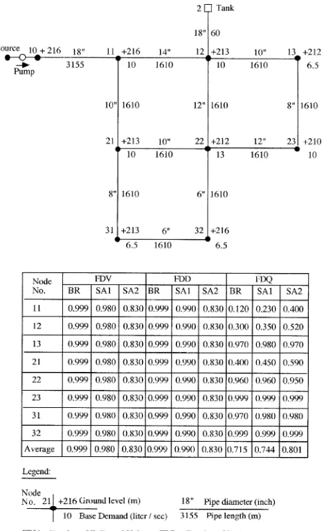
The proposed methodology is demonstrated on a small illustrative system (Example 1, Rossman, 1994). The system data, and the outcome of a Base Run and two sensitivity analysis reliability runs are shown in Fig. 3. The system consists of 12 pipes, a source, a pump, and an elevated storage tank. The system is subject to a 24-h representative demand pattern as in Table 1.

The pump is fed by a source that is at a constant water level of 243.8 m. The water is delivered to a storage elevated tank at node 2 (at a ground level of 259.1 m), and to eight consumers located at nodes 11, 12, 13, 21, 22, 23, 31, and 32. The pump has a shutoff

head value of 101.3m, a 189.3l=s maximum flow rate,

The pump is ‘‘on’’ if the water level at the storage tank (above ground) is below 33.5 m, and is ‘‘off ’’ if the water level is above 42.7 m. The tank is cylindrical with a

diameter of 15.4 m. Its minimum, initial, and maximum levels, above ground, are 30.5, 36.6 and 45.7 m, re-spectively.

The data required for the reliability simulation runs are shown in Table 2.

4.1.1. Base Run

The Base Run (and two sensitivity analysis) results for Example 1 are shown in Fig. 3. The Base Run in-cluded a relatively small probability for system failure: 0.01, resembling ‘‘real’’ system operation, and a system maximum time of repair (MTOR) of 8 h.

The system has failed seven times out of the 1000 simulations conducted (i.e. approximately 1% of the runs, as expected with a system failure probability of 0.01). The components outages: type, time of occurrence during the day, and duration of repair, are shown in Table 3.

As expected, since the system can be supplied from both the source and the elevated tank, and since each consumer can be reached by at least two alternate paths,

the reliability at each of the consumers is 1.0 for the

FDV and FDD measures. However, with respect to FDQ, since the initial source concentration is 300

(mg=l), and the consumers threshold concentration

re-quest is 200 (mg=l), the worst FDQ is at node 11 (near

the source), which improves gradually towards the far-most consumers (22, 23, 31, and 32) as dilution domi-nates. The average FDQ measure (i.e. the average FDQ of all eight consumers) is 0.715.

4.1.2. Sensitivity analysis 1

The objective of sensitivity analysis 1 (and 2 that follows) is to explore the system response to changes made in the data. In sensitivity analysis 1 a bound for the system reliability was taken to an extreme, by making the probability of the system being in a failure mode as 1.0 (i.e. at each simulation run one of the system components was randomly out of service), keeping all other data as in the Base Run. The average FDV and FDD measures were lowered to 0.98 and 0.99, respectively, while the average FDQ was 0.744.

4.1.3. Sensitivity analysis 2

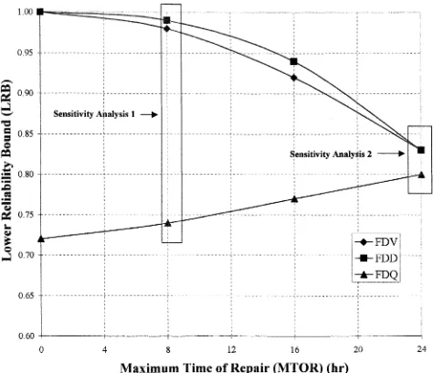
In sensitivity analysis 2 the probability of system failure was kept at 1.0, and the MTOR has been ex-tended to 24 h. The average FDV and FDD measures were lowered to 0.83, while the average FDQ was 0.801. Fig. 4 shows the trade-off between the MTOR, and the average lower reliability bounds (LRB) of the system FDV, FDD, and FDQ, generated by taking the proba-bility of the system being in a failure mode as 1.0. For

MTOR¼0, LRB is 1 for FDV and FDD. For

MTOR¼8 and 24 h, the LRBs are the average of the

values shown in Fig. 3.

Fig. 3. Example 1 (Rossman, 1994): data, and reliability analysis re-sults.

Table 1

24-h demand pattern characteristics for Example 1 (Rossman, 1994)

Time of day Multiplier of base demand

24–2 1.0

2–4 1.2

4–6 1.4

6–8 1.6

8–10 1.4

10–12 1.2

12–14 1.0

14–16 0.8

16–18 0.6

18–20 0.4

20–22 0.6

As expected (see Fig. 3), FDD is always greater than or equal to FDV, as FDV accumulates all shortages, while FDD accumulates shortages only after reaching a threshold bound. What is not expected is the rise of FDQ with MTOR. This can be explained by the fact that the probability taken for the source and

the pump being out of service is 0.1, and 0.6 respec-tively, while that of a pipe: 0.3(see Table 2). As an outcome of that, at most of the outages (five out of seven, see Table 3) the source was out of service, and the consumers were supplied by the tank whose initial

concentration was 1.0 (mg=l). Thus, as the MTOR

extended, the consumers received better water quality, but at much lower quantities (i.e. the FDV and FDD were lowered much faster than the raise of FDQ, as shown in Fig. 4).

4.2. Example 2

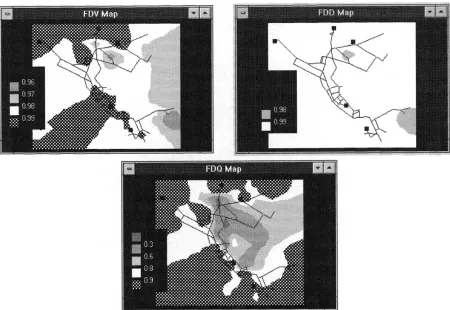
In this example, the outcome of RAP is demonstrated on a ‘‘real-life’’ network (Fig. 5) – Example 3of EPA-NET (Rossman, 1994). The system consists of two sources, three elevated tanks, 117 pipes, 97 demand nodes, and two pumps (the complete data used was exactly as that of Example 3, in Rossman (1994), and thus is not repeated here).

The FDV, FDD, and FDQ maps of a Base Run are shown in Fig. 6. The gray scale hues in Fig. 6 represent domains of reliability values. Such maps can be used to identify portions of the system with low reliability val-ues, and thus in general for visual comparisons (note that the colors in Fig. 6 are applicable only where a water distribution system exists, there is no physical meaning outside of the system).

Table 2

Reliability simulation data for Example 1 (Rossman, 1994): Base Run and sensitivity analysis

Base Run Sensitivity analysis 1 Sensitivity analysis 2

Fluctuations from average demand 0.1 0.1 0.1

Probability of system failure 0.01 1.0 1.0

Probability of pump failure (given the system is in a failure mode) 0.6 0.6 0.6

Probability of pipe failure (given the system is in a failure mode) 0.30.3 0.3 Probability of source failure (given the system is in a failure mode) 0.1 0.1 0.1

Maximum time of repair (h) 8 8 24

Number of simulation runs 1000 1000 1000

Threshold demand factor 0.9 0.9 0.9

Quality fluctuation at sources: min, max 0.1, 0.2 0.1, 0.2 0.1, 0.2

Threshold quality factor 0.1 0.1 0.1

Initial source concentration (mg=l) 300 300 300

Initial tank concentration (mg=l) 1.0 1.0 1.0

Consumers threshold concentration demands (mg=l) 200 200 200

Table 3

Components outages for Example 1 (Rossman, 1994): type, time of occurrence during the day, and duration of repair

Run number Component type Time of outage Duration of repair (h)

348 Pump 21:00 1.0

422 Pump 20:00 7.0

461 Pump 17:00 1.0

630 Pump 18:00 5.0

654 Pipe connecting nodes 10 and 11 21:00 7.0

787 Pump 19:00 1.0

944 Pipe connecting nodes 11 and 21 6:00 5.0

As in Example 1, it can be clearly seen that FDD is always greater or equal FDV, and that FDQ greatly depends on the water quality distribution at the sources, and on the consumers water quality demands, and less on the hydraulic reliability of the system.

In summary, it is hard to find a clear connection between FDV (or FDD), representing the hydraulic re-liability of the system, and FDQ.

5. Conclusions

Reliability analysis of water distribution systems is a complex task as it requires both the definition and cal-culation of reliability measures. This paper has demon-strated an application of stochastic simulation for reliability analysis of water distribution systems, taking into account the quality of the water supplied, as well as hydraulic reliability considerations. The model is limited to one random component failure at a time, uniform time to failure and time to repair probability distribu-tion funcdistribu-tions (a simplificadistribu-tion of the real world time to failure and time to repair PDFs), a square root ‘‘pressure–demand’’ relationship (Wagner et al., 1988a), and is expensive to run. In addition, the model does not take into account the impact of the valves topology (e.g. Walski, 1993) on the system isolated portions – once a failure occurs, and the systems fire fighting capacity demand. Nevertheless, the results obtained in example analyses were able to quantify the reliability of the

sys-Fig. 5. Example 2 (Example 3of Rossman, 1994).

tems and to generate bounds for the reliability measures adopted.

Acknowledgements

This work was funded by the Water Research Insti-tute (WRI) at the Technion, Israel InstiInsti-tute of Tech-nology. The support of the WRI is highly acknowledged.

References

Bao, Y., & Mays, L. W. (1990). Model for water distribution system reliability.Journal of Hydraulic Engineering,116(9), 1119–1137. Cohen, D., Shamir, U., & Sinai, G. (1999a). Optimal operation of

multi-quality networks – I: Introduction and the Q–C model. Engineering Optimization,32(5), 549–584.

Cohen, D., Shamir, U., & Sinai, G. (1999b). Optimal operation of multi-quality networks – II: The Q–H model.Engineering Optimi-zation,32(6), 687–719.

Cohen, D., Shamir, U., & Sinai, G. (2000). Optimal operation of multi-quality networks – III: The Q–C–H model.Engineering Optimiza-tion,33(1), 1–35.

Engelhardt, M. O., Skipworth, P. J., Savic, D. A., Saul, A. J., & Walters, G. A. (2000). Rehabilitation strategies for water distribu-tion networks: a literature review with a UK perspective.Urban Water,2(2), 153–170.

Fujiwara, O., & Ganesharajah, T. (1993). Reliability assessment of water supply systems with storage and distribution networks. Water Resources Research,29(8), 2917–2924.

Liang, T., & Nahaji, S. (1983). Managing water quality by mixing water from different sources.Journal of Water Resources Planning and Management Division,109, 48–57.

Mays, L. W. (Ed.) (1989). Reliability analysis of water distribution systems, Congress Cataloging-in-Publication Data, American So-ciety of Civil Engineers, 532 pp.

Ostfeld, A., & Shamir, U. (1996). Design of optimal reliable multiq-uality water supply systems.Journal of Water Resources Planning and Management Division,122(5), 322–333.

Quimpo, R. G., & Shamsi, U. M. (1991). Reliability based distribution system maintenance. Journal of Water Resources Planning and Management Division,117(3), 321–339.

Rossman, L. A. (1994). EPANET User Manual, Risk Reduction Engineering Laboratory, US Environmental Protection Agency, Cincinnati, OH, 107 pp; www.epa.gov/ORD/NRMRL/wswrd/ epanet.html.

Shamsi, U. (1990). Computerized evaluation of water supply reliabil-ity.IEEE Transaction on Reliability,39(1), 35–41.

Sinai, G., Koch, E., & Farbman, M. (1985). Dilution of brakish waters in irrigation networks – an analytic approach.Irrigation Science,6, 191–200.

Su, Y. C., Mays, L. W., Duan, N., & Lansey, K. E. (1987). Reliability-based optimization model for water distribution systems.Journal of Hydraulic Engineering,114(12), 1539–1556.

Wagner, J. M., Shamir, U., & Marks, D. H. (1988a). Water distribution reliability: Analytical methods. Journal of Water Resources Planning and Management Division,114(3), 253–275. Wagner, J. M., Shamir, U., & Marks, D. H. (1988b). Water

distribution reliability: Simulation methods. Journal of Water Resources Planning and Management Division,114(3), 276–294. Walski, T. M. (1993). Water distribution valve topology for