Ames Laboratory Accepted Manuscripts
Ames Laboratory
11-1-2017
Determining the vortex tilt relative to a
superconductor surface
Vladimir G. Kogan
Ames Laboratory, [email protected]
J. R. Kirtley
Stanford UniversityFollow this and additional works at:
http://lib.dr.iastate.edu/ameslab_manuscripts
Part of the
Condensed Matter Physics Commons
, and the
Materials Science and Engineering
Commons
This Article is brought to you for free and open access by the Ames Laboratory at Iowa State University Digital Repository. It has been accepted for inclusion in Ames Laboratory Accepted Manuscripts by an authorized administrator of Iowa State University Digital Repository. For more information, please [email protected].
Recommended Citation
Kogan, Vladimir G. and Kirtley, J. R., "Determining the vortex tilt relative to a superconductor surface" (2017).Ames Laboratory Accepted Manuscripts. 71.
Determining the vortex tilt relative to a superconductor surface
Abstract
It is of interest to determine the exit angle of a vortex from a superconductor surface, since this affects the
intervortex interactions and their consequences. Two ways to determine this angle are to image the vortex
magnetic fields above the surface, or the vortex core shape at the surface. In this work we evaluate the field
h(x,y,z) above a flat superconducting surface x,y and the currents J(x,y) at that surface for a straight vortex
tilted relative to the normal to the surface, for both the isotropic and anisotropic cases. In principle, these
results can be used to determine the vortex exit tilt angle from analyses of magnetic field imaging or density of
states data.
Disciplines
Condensed Matter Physics | Materials Science and Engineering
PHYSICAL REVIEW B96, 174516 (2017)
Determining the vortex tilt relative to a superconductor surface
V. G. Kogan
Ames Laboratory DOE and Iowa State University, Ames, Iowa 50011, USA
J. R. Kirtley
Geballe Laboratory for Advanced Materials, Stanford University, Stanford, California 94305, USA
(Received 16 June 2017; revised manuscript received 12 November 2017; published 20 November 2017)
It is of interest to determine the exit angle of a vortex from a superconductor surface, since this affects the intervortex interactions and their consequences. Two ways to determine this angle are to image the vortex magnetic fields above the surface, or the vortex core shape at the surface. In this work we evaluate the field
h(x,y,z) above a flat superconducting surfacex,yand the currents J(x,y) at that surface for a straight vortex tilted relative to the normal to the surface, for both the isotropic and anisotropic cases. In principle, these results can be used to determine the vortex exit tilt angle from analyses of magnetic field imaging or density of states data.
DOI:10.1103/PhysRevB.96.174516
I. INTRODUCTION
In the long history of studying vortices and vortex lattices with the help of surface probes [e.g., Bitter decoration [1,2], Hall bar microscopy [3], magnetic force microscopy [4], scanning superconducting quantum interference device (SQUID) microscopy (SSM) [5], or scanning tunneling mi-croscopy (STM) [6]], vortices were commonly assumed to exit the superconductor perpendicular to the surface. Hess and collaborators were the first to examine vortex lattices in NbSe2 in tilted fields [6] using STM. They found a peculiar
“cometlike” density of states (DOS) distribution near the vortex core. Recently, the STM group of Suderow concluded that the vortex lattice structure in fields tilted relative to a plane surface of nearly isotropicβ-Bi2Pd is affected by the surface
contribution to the vortex-vortex interactions due to vortex stray fields outside the sample [7].
The question then arises as to whether one can determine the vortex orientation relative to the surface by measuring the field above the sample surface or the DOS at the surface for a superconductor containing vortices. This question is addressed in this paper.
There has already been a great deal of work on the structure of vortices near and above a sample surface. Abrikosov [8] used Ginzburg-Landau theory to determine the structure of a vortex lattice in a bulk, isotropic superconductor. Pearl calculated the current distribution of quantized fluxoids in superconducting thin films [9] and the currents and fields of vortices near and above a superconductor-vacuum interface [10]. Brandt [11] described a method for calculating the properties of a distorted flux line lattice near a planar surface using the London theory. Buisson et al. [12] generalized this study for the case of mass anisotropy orthogonal to the surface. Kogan, Simonov, and Ledvij (KSL) [13] considered a uniaxial crystal with a surface in an arbitrary crystal plane and a vortex with arbitrary orientation relative to the crystal within the general anisotropic London approach. Carneiro and Brandt [14] gave general expressions for the magnetic field and energy of straight and curved vortices in an anisotropic superconductor of finite thickness within anisotropic London theory.
Here, we apply the formalism of KSL [13] to the problem of currents near and fields above the surface for a tilted vortex in an anisotropic superconductor. The KSL formalism is quite general, but this “generality” make the results quite cumbersome and not easily applied. Besides, it is unclear which features of the field distribution outside, or of the DOS at the interface, are due to the vortex tilt and which are due to crystal anisotropy.
For this reason, we focus here first on the isotropic half-space superconductor at z <0 and a straight vortex approaching the interfacez=0 at an angleθwith the normal ˆ
zto the surface. Forθ =0 this problem has been solved by Pearl [10]. We find that even in the isotropic case, the field distribution above the surface and the currentsJ(x,y) flowing at the surface carry measurable signs of the vortex tilt. The stray fieldhz(x,y;z) can, in principle, be measured by field sensitive
probes such as scanning Hall bar or scanning SQUID, whereas |J(x,y)|affects the pair potential and DOS probed by STM.
In the second part of this paper, we consider tilted vortices in uniaxial superconductors with the surface in theabplane.
II. ISOTROPIC CASE
The formal method we use is straightforward and not new: One solves the London equations inside the superconductor, the Maxwell equations outside, and match the solutions with proper boundary conditions [10,12–15].
The field h outside the superconductor satisfies divh=
curlh=0, so that one can look for this field ash=∇ϕwith the potential ϕ obeying the Laplace equation ϕ=0. The general solution of this equation in the upper half spacez >0 forϕ→0 asz→ ∞is
ϕ(r,z)=
d2k
4π2ϕ(k)e
ikr−kz,
(1)
where
ϕ(k,z)=
d2rϕ(r,z)e−ikr−kz (2)
is the two-dimensional (2D) Fourier transform of the potential
ϕ,r=(x,y),k=(kx,ky).
V. G. KOGAN AND J. R. KIRTLEY PHYSICAL REVIEW B96, 174516 (2017)
Inside the superconductor, the field components satisfy the London equations
hi−λ2hi=0vˆiδ(x0,y0). (3)
Here, = ∇2+∂2/∂z2 with the 2D Laplacian ∇2; ˆv is
the unit vector along the vortex axis, and (x0,y0) are the coordinates in the plane perpendicular to the vortex axis ˆv. For an infinite vortex alongz0in uniform material, the coordinates
(x0,y0,z0) are the best, because nothing depends on z0. In
the case of a vortex crossing the surface of superconducting half space, this feature is lost, and the coordinates (x,y,z) with z=0 being the sample surface are more convenient. The delta function at the right-hand side (RHS) becomes
δ(x0)δ(y0)=δ(xcosθ−zsinθ)δ(y), where θ is the angle
between z andv, the “tilt” angle, and they axis is chosen to havevy =0.
The solution of the system (3) of linear differential equations is the sum of its particular solution and of the solutionhsof the homogeneous equation with zero RHS. To have a correct singular behavior at the vortex axis, we choose the particular solution as the well-known field of an infinite straight vortexhv:
h=hv+hs. (4)
After taking a 2Dx,yFourier transform of Eq. (3), one obtains atz=0 (see Appendix A of Ref. [15]):
hvx(k)= 0tanθ
λ2Q2 , h
v
y =0, h v z(k)=
0
λ2Q2, (5)
Q2 =λ−2+k2+kx2tan2θ. (6)
Further, the 2D Fourier transform turns the homogeneous Eq. (3) into a system of ordinary differential equations for
hsi(k,z) in the variablez,
hsiλ−2+k2hsi−∂2hsi/∂z2=0, (7)
with solutions
hsi(k,z)=Hi(k)eqz, q2=λ−2+k2. (8)
Note that all components of hs decay exponentially with the characteristic length 1/q =λ/√1+λ2k2.
Note also that Hi are not independent: By choosing the
particular solution as the field of an infinite vortex which obeys divhv =0, we impose the same condition onhs,
ikxHx+ikyHy+qHz=0. (9)
The boundary conditions of the field continuity atz=0 read inkspace,
ikxϕ =hvx+h s x,
ikyϕ =hvy+h s
y, (10)
−kϕ =hvz+hsz.
Along with Eqs. (5) and (9) these conditions give for the external potential
ϕ(k,z)= − 0e
−kz
λ2k(k+q)(q−ik
xtanθ)
[image:4.608.312.558.69.266.2], (11)
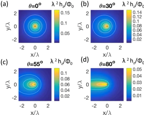
FIG. 1. Normalizedzcomponent of the magnetic fieldsλ2h z/0
at heightz=0.1λabove a superconducting surface for a tilted vortex in the isotropic case. The contours of constant hz (white) are at
λ2h
z/0=0.02, 0.04, 0.06, 0.08, 0.10, and 0.12. The “+” symbols
mark the centers of the vortex coordinate system where the vortex axis touches the surface.
and for the coefficientsHi,
Hx = −0
k2
y+kq
tanθ+ikxq
λ2k(k+q)Q2 ,
Hy = −0
iky(ikxtanθ+q)
λ2k(k+q)Q2 , (12)
Hz=0
ikxtanθ−k
λ2(k+q)Q2.
A. Distribution of the fieldhz(x,y;z)
From the potential (11) we get thezcomponent of the field outside,
hz(k,z)=
0e−kz
λ2(k+q)(q−ik
xtanθ)
. (13)
In principle, this field can be measured in scanning Hall bar or SQUID experiments. Figure1 shows results of numerical inversion of this Fourier transform to real space. The vortex fields above the sample surface become weaker and more elongated in the tilt (x) direction as the tilt angle increases.
To characterize asymmetry of the fieldhzfor tilted vortices,
we plot in Fig. 2 the fields hz(x,0) for the tilts of Fig. 1.
Clearly, asymmetry increases with increasingθ. A simple way to quantify this asymmetry is to consider the half width of domelike curveshz(x,0) as consisting of two parts,aandb,
separated by the position of the curve maximum (see Fig.2). For θ=0, hz(x,0)=hz(−x,0), and b−a =0. Since the
angleθentershz(k,θ) only via tanθ, we plota−bvs tanθto
see that in a broad domain of angles (b−a)∝tanθ. In fact, Fig.2forz=0.1λsuggests an empirical relation (b−a)≈ 0.5λtanθ. Thus, by measuring the asymmetryb−a one can estimate the tilt angleθ.
DETERMINING THE VORTEX TILT RELATIVE TO A . . . PHYSICAL REVIEW B96, 174516 (2017)
-3 -2 -1 0 1 2 3
x/ 0 0.02 0.04 0.06 0.08 0.1 0.12 0.14 0.16 0.18
2 h
z / 0 =0o 30o 55o 70o
0 1 2 3
tan( ) 0 0.5 1 1.5 (b-a)/
-5 0 5
x/ 0
[image:5.608.309.557.69.261.2]05 .1
FIG. 2. Normalizedzcomponent of the magnetic fieldshz(x,0) at
heightz=0.1λabove the surface for tilted vortices in the isotropic case. Inset (a): Definitions of a and bto characterize the curves’ asymmetry. Inset (b):b−avs tanθ extracted from curves in the main panel.
B. SupercurrentsJ(x,y) at the surface
Supercurrents flowing at the surface affect the order param-eter and the DOS measured by STM. It is not easy to track this connection for arbitrary temperatures. For a qualitative argument we can use the Ginzburg-Landau theory which gives a simple relation for the order parameter suppression by current,2=2
0(1−J2/4Jd2), where0corresponds to zero
current andJd =c0/16π2λ2ξis on the order of the depairing
current (ξ is the coherence length) [16]. According to de Gennes, the zero-bias density of statesNin the vortex vicinity is related to the order parameter asN(r)/N0=1−2(r)/20
[17]. This suggests that the contoursJ2(x,y)=const should
be close to the DOS contoursN(x,y)=const. Of course, the London approach employed here cannot be trusted at distances on the order ξ, where the current approaches the depairing value. Still, being interested in a qualitative description of the vortex core shape at the sample surface, one can study the functionJ2(x,y).
The part of the current at z=0 associated with the unperturbed tilted vortex has been given in Ref. [15],
Jxv(k)= c0 4π λ2
iky
Q2, (14)
Jyv(k)= −c0 4π λ2
ikx
Q2cos2θ. (15)
The contribution to the current due to the fieldhsof Eq. (8)
atz=0 follows from Maxwell’s equations,
4π c J
s
x(k)=ikyHz(k)−qHy(k), (16)
4π c J
s
y(k)=qHx(k)−ikxHz(k). (17)
It is worth noting that the continuity of the tangential fields
hx,yassures also the continuity of their tangential derivatives,
[image:5.608.53.294.70.252.2]in other words, the continuity of the normal current component
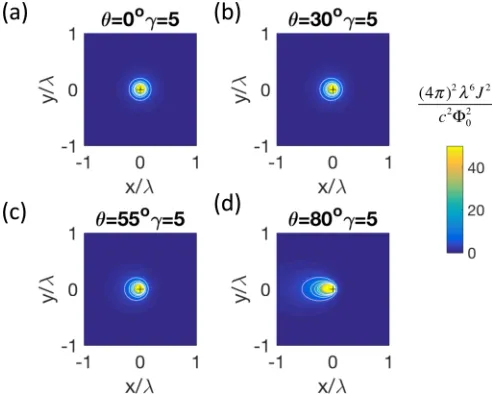
FIG. 3. Normalized absolute value squared of the vortex currents (4π)2λ6J2/c22
0at the superconducting surface in the isotropic case.
The tilt angle of the vortex relative to the sample surfaceθ=0◦(a), 30◦(b), 55◦(c), and 80◦(d). The contours of constantJ2(white) are
at (4π)2λ6J2/c22
0=1, 2, 3, 4, and 5. The “+” symbol marks the
center of the vortex coordinate system where the vortex axis touches the surface.
Jz. But Jz=0 outside the sample and so does the normal
component of the total current inside (Jv+Js)
z=0 at the
interface.
Hence, we can evaluate the current value at the surface in real space:
J2(x,y)=Jxs+Jxv2+Jys+Jyv2. (18)
Some numerical evaluations of Eq. (18) are displayed in Figs. 3 and 4. For these calculations we applied a
-1 -0.5 0 0.5 1
x/ 0 2 4 6 8 10 (4 ) 2
6 J 2 /c 2 0 2 =0o 30o 50o 70o
-1 0 1
0 5 10
0 1 2 3
tan( ) -0.1 0 0.1 0.2 (d-c)/
FIG. 4. Cross sections through y=0 of the vortex currents (4π)2λ6J2/c22
0at the superconducting surface in the isotropic case.
The tilt angle of the vortex relative to the sample surfaceθ=0◦, 30◦, 55◦, and 70◦. Inset (a) definescandd, the values of|x|when (4π)2λ6J2/c22
0=10. Inset (b) plotsd−cas a function of tan(θ).
[image:5.608.315.557.499.688.2]V. G. KOGAN AND J. R. KIRTLEY PHYSICAL REVIEW B96, 174516 (2017)
high frequency filter by multiplying the right-hand sides of Eqs. (14)–(17) by e−k2dz2
with dz=0.01λ. This damps out high frequency artifacts at x=0 and y =0 without significantly effecting the low frequency properties of the solutions. The false color scale in Fig. 3 is saturated at (4π)2λ6J2/c22
0=10. Since physically the core shape (as
observed in, e.g., STM) is determined by a contour whereJ
reaches the depairing value, the contoursJ2(x,y)=const will
also give the contours of DOS(x,y)=const: The observed vortex cores will become more elongated along the tilt (x) direction as the tilt angle increases. To avoid misunderstanding, we stress that the white curves in Fig.3are contoursJ2(x,y)=
const, not the stream lines of the vector J(x,y).
Figure4plots cross sections throughy =0 of the calculated vortex currents of Fig.3in the isotropic case for various vortex tilt angles θ. The inset Fig. 4(a) diagrams the intercepts c
andd where ¯j2≡(4π)2λ6J2/c22
0=10. Figure 4(b) plots
(d−c)/λ, a measure of the asymmetry of the vortex currents at the surface, as a function of tanθ. The vortex current asymmetry varies roughly linearly with tanθ, as does the vortex field asymmetry (Fig.2). When we fit the vortex current asymmetry to the expression (d−c)/λ=a1tanθ+a2 for
various values of ¯j2, we find the empirical relationa
1=α/j¯
withα=0.335±0.004. One can in principle determine the vortex tilt angle from the vortex current asymmetry using this relation.
III. UNIAXIAL CRYSTAL WITH SURFACE ATabPLANE
The general case of an anisotropic half-space supercon-ductor with an arbitrary plane surface and arbitrarily oriented vortex has been considered in Ref. [13]. Here, we are interested in the surface coinciding with the ab plane (Sec. III A of Ref. [13]). In this case, the coordinatesx,y,zcoincide with the crystal’sa,b,caxes, and the mass tensor is diagonal,mxx =
myy=ma,mzz=mc, the “effective masses” are normalized
m2amc=1, and the anisotropy parameter γ =
√
mc/ma =
λc/λab.
The basic scheme of the solution is the same as in the isotropic case: One has to solve the anisotropic London equations [18] inside and to match them to solutions of the Maxwell equations for the field outside. Without going into formal details (for which readers are referred to Ref. [13]) we note a relevant point: While solving the system of London equations for the surface contribution to the internal field in the form hs
i(k,z)=Hi(k)eqz, we obtain a system of linear
homogeneous equations forHi(k), the determinant of which
must be zero. This gives possible values of the parameterq. After straightforward algebra one obtains two positive roots,
q1=
λ−2ab +k2, q 2=
λ−2ab +γ2k2. (19)
Hence, instead of one mode of the field decay of the isotropic case, we have now two such modes. The prefactors H(1)and
H(2)are given by
Hx(1)=Hy(1)kx ky =
Hz(1)ikxq1
k2 , (20)
Hz(1)=0
ikxtanθ−k
(k+q1)d1
, (21)
d1=1+λ2abk2+kx2tan2θ, (22)
Hx(2)= −Hy(2)ky kx
= −0 k2
ytanθ
k2d 2
, Hz(2)=0, (23)
d2 =1+λ2ck2+λ2abkx2tan2θ. (24)
The boundary conditions of the field continuity atz=0 now read
ikxϕ =hvx+Hx(1)+Hx(2), (25)
ikyϕ =hvy+H
(1)
y +H
(2)
y , (26)
−kϕ=hvz+Hz(1). (27)
The 2D Fourier components of the fieldhv atz=0 are
given in Appendix A of Ref. [15]:
hvx =0tanθ
1+λ2abkx2tan2θ+ky2+λ2ckx2/d, (28)
hvy =0tanθ
λ2c−λ2abkxky/d, (29)
hvz=0/
1+λ2abkx2sec2θ+ky2, d =d1d2. (30)
The condition divhs=0 atz=0 translates toik
x(Hx(1)+
H(2)
x )+iky(Hy(1)+Hy(2))+q1Hz(1)=0, so that one easily
excludes allH’s from the system (25)–(27) to obtain
ϕ = − 0e
−kz
λ2abk(k+q1)(q1−ikxtanθ)
(31)
Note thatλcdoes not enter this expression. Hence, the outside
field depends only onλab. It is worth noting that if the vortex
as the field source is replaced with some external source, the response field outside also does not depend onλc[19].
From the potential we get
hz= −kϕ(k)=
0e−kz
λ2
ab(k+q1)(q1−ikxtanθ)
. (32)
Fork→0,q1=1/λab, so that the total fluxhz(k=0)=0,
as it should.
Surface currents
As before, the current consists of the vortex and surface contributions,JvandJs. The surface contribution is given by
4π c J
s
x(k)=ikyHz(1)−q1Hy(1)−q2Hy(2), (33)
4π c J
s
y(k)=q1Hx(1)+q2Hx(2)−ikxHz(1). (34)
For a tilted vortex, the currents at the surface are given in Appendix A of Ref. [15]:
4π c J
v x =0
iky
1+λ2ck2+k2xtan2θ d1d2
, (35)
4π c J
v y = −0
ikx
1+λ2
ab(sin2θ+γ2cos2θ)
k2+k2
xtan2θ
d1d2cos2θ .
(36)
DETERMINING THE VORTEX TILT RELATIVE TO A . . . PHYSICAL REVIEW B96, 174516 (2017)
FIG. 5. Normalized absolute value squared of the vortex currents (4π)2λ6J2/c22
0 at the superconducting surface in the uniaxial
anisotropic case with γ =5. The tilt angle of the vortex relative to the sample surfaceθ=0◦(a), 30◦ (b), 55◦(c), and 80◦(d). The false color map is saturated at (4π)2λ6J2/c22
0=50. The contours
of constantJ2(white) are at (4π)2λ6J2/c22
0=5, 10, 15, 20, and 25.
The “+” symbol marks the center of the vortex coordinate system.
One can now evaluate numerically J2(x,y)=(Js x +
Jv
x)2+(Jys+Jyv)2at the surface. Results are shown in Fig.5.
We again applied a high frequency filtere−k2dz2
withdz=
0.01λ to damp out high frequency oscillations at x=0 and y=0. The false color scale in Fig. 5 is saturated at (4π)2λ6J2/c220=50. Note that the current densities are higher and the elongation of the vortex core along the tilt axis at high tilt angles is less pronounced as compared with the isotropic case (Fig.3).
The systematic behavior of the vortex core with uniaxial anisotropy is illustrated in Fig.6.
IV. DISCUSSION
[image:7.608.317.555.70.269.2]Numerical analysis of the expressions given above show that the external magnetic fields from vortices become weaker as the tilt angle increases, at the same time as the vortex shape becomes more elongated in the tilt direction (Fig.1). In contrast, the peak absolute values of the surface supercurrents are relatively insensitive to tilt angle, while the vortex core elongation increases with tilt angle (Fig. 3). For a uniaxial superconductor the surface currents become stronger with higher anisotropy, but the vortex cores become less elongated (Figs. 5 and6). This, at first sight, is surprising but could be understood qualitatively by comparing tilted vortices near the surface in the isotropic and anisotropic cases. Since there the currents must be parallel to the surface, in isotropic
FIG. 6. Normalized absolute value squared of the vortex currents (4π)2λ6J2/γ c22
0 at the superconducting surface in the uniaxial
anisotropic case for a tilt angle of 80◦. The anisotropy parameter is
γ=1 (a), 2 (b), 5 (c), and 10 (d). The false color scales are saturated at (4π)2λ6J2/γ c22
0=10. The contours of constantJ2(white) are at
(4π)2λ6J2/γ c22
0=1, 2, 3, 4, 5. The “+” symbol marks the center
of the vortex coordinate system.
materials the surface causes a strong distortion of the currents in its vicinity as compared to the bulk. On the other hand, in an anisotropic uniaxial sample with the ab surface, the unperturbed bulk current planes are already tilted towardab
due to anisotropy, so that the distortion caused by the surface is getting weaker with increasing anisotropy. In the limitγ 1, the surface distortion disappears altogether, which we in fact see in our simulations.
Experimental tests of these effects would be a challenge with existing trilayer [20] or Dayem bridge [21] SQUID microscopes, which have spatial resolution of somewhat less than 1μm, while superconducting penetration depths are typically 0.1μm. However, recent SQUID-on-a-tip sensors [22] may have the spatial resolution required. Of course, STM easily has the spatial resolution to look for the vortex elongations predicted here.
ACKNOWLEDGMENTS
The authors thank Herman Suderow and Christophe Berthod for helpful discussions. V.K. was supported by the U.S. Department of Energy, Office of Science, Basic Energy Sciences, Materials Sciences and Engineering Division. The Ames Laboratory is operated for the U.S. DOE by Iowa State University under Contract No. DE-AC02-07CH11358. J.K. was supported by Stanford University.
[1] U. Essman and H. Träuble, Phys. Lett. A 24, 526
(1967).
[2] G. J. Dolan, F. Holtzberg, C. Feild, and T. R. Dinger,Phys. Rev. Lett.62,2184(1989).
V. G. KOGAN AND J. R. KIRTLEY PHYSICAL REVIEW B96, 174516 (2017)
[3] A. M. Chang, H. D. Hallen, L. Harriott, H. F. Hess, H. L. Kao, J. Kwo, R. E. Miller, R. Wolfe, J. Van der Ziel, and T. Y. Chang,
Appl. Phys. Lett.61,1974(1992).
[4] H. J. Hug, A. Moser, I. Parashikov, B. Stiefel, O. Fritz, H. J. Güntherodt, and H. Thomas,Physica C235,2695(1994). [5] J. R. Kirtley,Rep. Prog. Phys.73,126501(2010).
[6] H. F. Hess, C. A. Murray, and J. V. Waszczak,Phys. Rev. B50,
16528(1994).
[7] E. Herrera, I. Guillamon, J. A. Galvis, A. Correa, A. Fente, S. Vieira, H. Suderow, A. Yu. Martynovich, and V. G. Kogan,Phys. Rev. B96,184502(2017).
[8] A. A. Abrikosov, Zh. Eksp. Teor. Fiz. 32, 1442 (1957) [Sov. Phys. JETP5, 1174 (1957)].
[9] J. Pearl,Appl. Phys. Lett.5,65(1964). [10] J. Pearl,J. Appl. Phys.37,4139(1966).
[11] E. H. Brandt,J. Low Temp. Phys.42,557(1981).
[12] O. Buisson, G. Carneiro, and M. Doria,Physica C 185,1465
(1991).
[13] V. G. Kogan, A. Yu. Simonov, and M. Ledvij,Phys. Rev. B48,
392(1993).
[14] G. Carneiro and E. H. Brandt, Phys. Rev. B 61, 6370
(2000).
[15] L. N. Bulaevskii, M. Ledvij, and V. G. Kogan,Phys. Rev. B46,
366(1992).
[16] A. A. Abrikosov,Fundamentals of the Theory of Metals (North-Holland/Elsevier, Amsterdam/New York, 1988).
[17] P. G. de Gennes, Phys. Kondens. Mater.3, 79 (1964). [18] V. G. Kogan,Phys. Rev. B24,1572(1981).
[19] V. G. Kogan,Phys. Rev. B68,104511(2003).
[20] J. R. Kirtley, L. Paulius, A. J. Rosenberg, J. C. Palmstrom, C. M. Holland, E. M. Spanton, D. Schiessl, C. L. Jermain, J. Gibbons, Y.-K.-K. Fung, M. E. Huber, D. C. Ralph, M. B. Ketchen, G. W. Gibson, Jr., and K. A. Moler, Rev. Sci. Instrum.87,
093702(2016).
[21] C. Veauvy, K. Hasselbach, and D. Mailly,Rev. Sci. Instrum.73,
3825(2002).
[22] D. Vasyukov, Y. Anahory, L. Embon, D. Halbertal, J. Cuppens, L. Ne’eman, A. Finkler, Y. Segev, Y. Myasoedov, M. L. Rappaport, M. E. Huber, and E. Zeldov,Nat. Nanotechnol.8,
639(2013).