chapter04-InstructionSets.pdf

(1)

CHAPTER 4 THE INSTRUCTION SET ARCHITECTURE 105

In this chapter we tackle a central topic in computer architecture: the language understood by the computer’s hardware, referred to as its machine language. The machine language is usually discussed in terms of its assembly language, which is functionally equivalent to the corresponding machine language except that the assembly language uses more intuitive names such as Move, Add, and Jump instead of the actual binary words of the language. (Programmers find con-structs such as “Add r0, r1, r2” to be more easily understood and rendered with-out error than 0110101110101101.)

We begin by describing the Instruction Set Architecture (ISA) view of the machine and its operations. The ISA view corresponds to the Assembly Lan-guage/Machine Code level described in Figure 1-4: it is between the High Level Language view, where little or none of the machine hardware is visible or of con-cern, and the Control level, where machine instructions are interpreted as regis-ter transfer actions, at the Functional Unit level.

In order to describe the nature of assembly language and assembly language pro-gramming, we choose as a model architecture the ARC machine, which is a sim-plification of the commercial SPARC architecture common to Sun computers. (Additional architectural models are covered in The Computer Architecture Com-panion volume.)

We illustrate the utility of the various instruction classes with practical examples of assembly language programming, and we conclude with a Case Study of the Java bytecodes as an example of a common, portable assembly language that can be implemented using the native language of another machine.

THE INSTRUCTION SET

ARCHITECTURE

(2)

106 CHAPTER 4 THE INSTRUCTION SET ARCHITECTURE

4.1 Hardware Components of the Instruction Set Architecture

The ISA of a computer presents the assembly language programmer with a view of the machine that includes all the programmer-accessible hardware, and the instructions that manipulate data within the hardware. In this section we look at the hardware components as viewed by the assembly language programmer. We begin with a discussion of the system as a whole: the CPU interacting with its internal (main) memory and performing input and output with the outside world.

4.1.1 THE SYSTEM BUS MODEL REVISITED

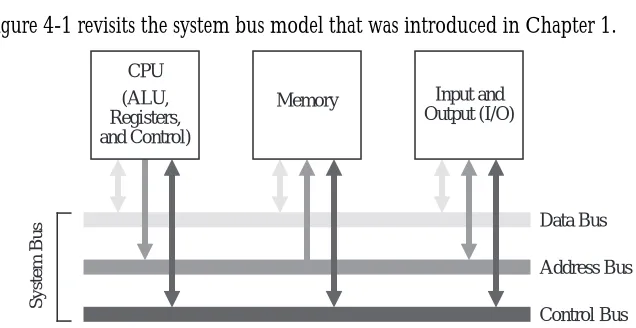
Figure 4-1 revisits the system bus model that was introduced in Chapter 1.

The purpose of the bus is to reduce the number of interconnections between the CPU and its subsystems. Rather than have separate communication paths between memory and each I/O device, the CPU is interconnected with its mem-ory and I/O systems via a shared system bus. In more complex systems there may be separate busses between the CPU and memory and CPU and I/O.

Not all of the components are connected to the system bus in the same way. The CPU generates addresses that are placed onto the address bus, and the memory receives addresses from the address bus. The memory never generates addresses, and the CPU never receives addresses, and so there are no corresponding connec-tions in those direcconnec-tions.

In a typical scenario, a user writes a high level program, which a compiler trans-lates into assembly language. An assembler then transtrans-lates the assembly language

System Bus

Data Bus

Address Bus

Control Bus (ALU,

Registers, and Control)

Memory Input and

Output (I/O) CPU

(3)

program into machine code, which is stored on a disk. Prior to execution, the machine code program is loaded from the disk into the main memory by an operating system.

During program execution, each instruction is brought into the ALU from the memory, one instruction at a time, along with any data that is needed to execute the instruction. The output of the program is placed on a device such as a video display, or a disk. All of these operations are orchestrated by a control unit, which we will explore in detail in Chapter 6. Communication among the three compo-nents (CPU, Memory, and I/O) is handled with busses.

An important consideration is that the instructions are executed inside of the ALU, even though all of the instructions and data are initially stored in the mem-ory. This means that instructions and data must be loaded from the memory into the ALU registers, and results must be stored back to the memory from the ALU registers.

4.1.2MEMORY

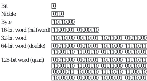
Computer memory consists of a collection of consecutively numbered (addressed) registers, each one of which normally holds one byte. A byte is a col-lection of eight bits (sometimes referred to by those in the computer communi-cations community as an octet). Each register has an address, referred to as a memory location. A nibble, or nybble, as it is sometimes spelled, refers to a col-lection of four adjacent bits. The meanings of the terms “bit,” “byte,” and “nib-ble” are generally agreed upon regardless of the specifics of an architecture, but the meaning of word depends upon the particular processor. Typical word sizes are 16, 32, 64, and 128 bits, with the 32-bit word size being the common form for ordinary computers these days, and the 64-bit word growing in popularity. In this text, words will be assumed to be 32-bits wide unless otherwise specified. A comparison of these data types is shown in Figure 4-2.

In a byte-addressable machine, the smallest object that can be referenced in memory is the byte, however, there are usually instructions that read and write multi-byte words. Multi-byte words are stored as a sequence of bytes, addressed by the byte of the word that has the lowest address. Most machines today have instructions that can access bytes, half-words, words, and double-words.

(4)

to as big-endian, or least significant byte stored at lowest address, referred to as little-endian. The term “endian” comes from the issue of whether eggs should be broken on the big or little end, which caused a war by bickering politicians in Jonathan Swift’s Gulliver’s Travels. Examples of big and little-endian formats for a 4-byte, 32-bit word is illustrated in Figure 4-3.

The bytes in a multi-byte word are stored at consecutive addresses, as shown in Figure 4-3. In a byte-addressable memory each byte is accessed by its specific address. The 4-byte word is accessed by referencing the address of the byte with the lowest address, x in Figure 4-3. This is true regardless of whether it is big-endian or little-endian. Since addresses are counted in sequence beginning with zero, the highest address is one less than the size of the memory. The highest address for a 232 byte memory is 232–1. The lowest address is 0.

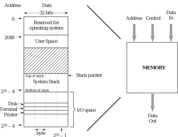
The example memory that we will use for the remainder of the chapter is shown in Figure 4-4. This memory has a 32-bit address space, which means that a pro-gram can access a byte of memory anywhere in the range from 0 to 232 – 1. The address space for our example architecture is divided into distinct regions which are used for the operating system, input and output (I/O), user programs, and

Bit Nibble Byte

16-bit word (halfword) 32-bit word

64-bit word (double) 0 0110 10110000

11001001 01000110

10110100 00110101 10011001 01011000 01011000 01010101 10110000 11110011 11001110 11101110 01111000 00110101 128-bit word (quad) 01011000 01010101 10110000 11110011 11001110 11101110 01111000 00110101 00001011 10100110 11110010 11100110 10100100 01000100 10100101 01010001 Figure 4-2 Common sizes for data types.

Big-Endian

x x+1 x+2 x+3

31 Little-Endian

x+3 x+2 x+1 x 0

Word address is x for both big-endian and little-endian formats.

0 31

Byte

← MSB LSB→ ← MSB LSB →

(5)

the system stack, which comprise the memory map, as shown in Figure 4-3. The memory map differs from one implementation to another, which is partly why programs compiled for the same type of processor may not be compatible across systems.

The lower 211 = 2048 addresses of the memory map are reserved for use by the operating system. The user space is where a user’s assembled program is loaded, and can grow during operation from location 2048 until it meets up with the system stack. The system stack starts at location 231 – 4 and grows toward lower addresses. The portion of the address space between 231 and 232 – 1 is reserved for I/O devices. The memory map is thus not entirely composed of real memory, and in fact there may be large gaps where neither real memory nor I/O devices exist. Since I/O devices are treated like memory locations, ordinary memory read and write commands can be used for reading and writing devices. This is referred to as memory mapped I/O.

It is important to keep the distinction clear between what is an address and what is data. An address in this example memory is 32 bits wide, and a word is also 32 bits wide, but they are not the same thing. An address is a pointer to a memory location, which holds data.

Reserved for operating system

User Space

I/O space 0

2048

Stack pointer System Stack

Top of stack

Bottom of stack

Disk Terminal Printer

232_{– 4} 231_{– 4}

32 bits

Address Data

232_{– 1} byte

MEMORY

Address Control

Data Out

Data In

(6)

In this chapter we assume that the computer’s memory is organized in a single address space. The term address space refers to the numerical range of memory addresses to which the CPU can refer. In Chapter 7 (Memory), we will see that there are other ways that memory can be organized, but for now, we assume that memory as seen by the CPU has a single range of addresses. What decides the size of that range? It is the size of a memory address that the CPU can place on the address bus during read and write operations. A memory address that is n bits wide can specify one of 2n items. This memory could be referred to as having an n-bit address space, or equivalently as having a (2n) byte address space. For exam-ple, a machine having a 32-bit address space will have a maximum capacity of 232 (4 GB) of memory. The memory addresses will range from 0 to 232- 1, which is 0 to 4,294,967,295 decimal, or in the easier to manipulate hexadecimal for-mat, from 00000000H to FFFFFFFFFH. (The ‘H’ indicates a hexadecimal number in many assembly languages.)

4.1.3 THE CPU

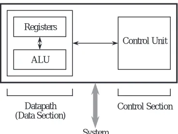
Now that we are familiar with the basic components of the system bus and mem-ory, we are ready to explore the internals of the CPU. At a minimum, the CPU consists of a data section that contains registers and an ALU, and a control sec-tion, which interprets instructions and effects register transfers, as illustrated in Figure 4-5. The data section is also referred to as the datapath.

The control unit of a computer is responsible for executing the program instruc-tions, which are stored in the main memory. (Here we will assume that the machine code is interpreted by the control unit one instruction at a time, though in Chapter 9 we shall see that many modern processors can process several

Control Unit

Control Section Registers

ALU

Datapath (Data Section)

(7)

instructions simultaneously.) There are two registers that form the interface between the control unit and the data unit, known as the program counter

(PC)† and the instruction register (IR). The PC contains the address of the instruction being executed. The instruction that is pointed to by the PC is fetched from the memory, and is stored in the IR where it is interpreted. The steps that the control unit carries out in executing a program are:

1) Fetch the next instruction to be executed from memory.

2) Decode the opcode.

3) Read operand(s) from main memory, if any.

4) Execute the instruction and store results.

5) Go to step 1.

This is known as the fetch-execute cycle.

The control unit is responsible for coordinating these different units in the exe-cution of a computer program. It can be thought of as a form of a “computer within a computer” in the sense that it makes decisions as to how the rest of the machine behaves. We will treat the control unit in detail in Chapter 6.

The datapath is made up of a collection of registers known as the register file and the arithmetic and logic unit (ALU), as shown in Figure 4-6. The figure depicts the datapath of an example processor we will use in the remainder of the chapter.

The register file in the figure can be thought of as a small, fast memory, separate from the system memory, which is used for temporary storage during computa-tion. Typical sizes for a register file range from a few to a few thousand registers. Like the system memory, each register in the register file is assigned an address in sequence starting from zero. These register “addresses” are much smaller than main memory addresses: a register file containing 32 registers would have only a 5-bit address, for example. The major differences between the register file and the system memory is that the register file is contained within the CPU, and is there-fore much faster. An instruction that operates on data from the register file can often run ten times faster than the same instruction that operates on data in

(8)

memory. For this reason, register-intensive programs are faster than the equiva-lent memory intensive programs, even if it takes more register operations to do the same tasks that would require fewer operations with the operands located in memory.

Notice that there are several busses inside the datapath of Figure 4-6. Three bus-ses connect the datapath to the system bus. This allows data to be transferred to and from main memory and the register file. Three additional busses connect the register file to the ALU. These busses allow two operands to be fetched from the register file simultaneously, which are operated on by the ALU, with the results returned to the register file.

The ALU implements a variety of binary (two-operand) and unary (one-oper-and) operations. Examples include add, and, not, or, and multiply. Operations and operands to be used during the operations are selected by the Control Unit. The two source operands are fetched from the register file onto busses labeled “Register Source 1 (rs1)” and “Register Source 2 (rs2).” The output from the ALU is placed on the bus labeled “Register Destination (rd),” where the results are conveyed back to the register file. In most systems these connections also include a path to the System Bus so that memory and devices can be accessed. This is shown as the three connections labeled “From Data Bus”, “To Data Bus”, and “To Address Bus.”

Register File

ALU From Data

Bus

To Data Bus To Address

Bus

Register Source 1 (rs1)

Register Source 2 (rs2)

Register Destination (rd)

Control Unit selects registers and ALU

function

Status to Control Unit

(9)

The Instruction Set

The instruction set is the collection of instructions that a processor can execute, and in effect, it defines the processor. The instruction sets for each processor type are completely different one from the other. They differ in the sizes of instruc-tions, the kind of operations they allow, the type of operands they operate on, and the types of results they provide.This incompatibility in instruction sets is in stark contrast to the compatibility of higher level languages such as C, Pascal, and Ada. Programs written in these higher level languages can run almost unchanged on many different processors if they are re-compiled for the target processor.

(One exception to this incompatibility of machine languages is programs com-piled into Java bytecodes, which are a machine language for a virtual machine. They will run unchanged on any processor that is running the Java Virtual Machine. The Java Virtual Machine, written in the assembly language of the tar-get machine, intercepts each Java byte code and executes it as if it were running on a Java hardware (“real”) machine. See the Case Study at the end of the chapter for more details.)

Because of this incompatibility among instruction sets, computer systems are often identified by the type of CPU that is incorporated into the computer sys-tem. The instruction set determines the programs the system can execute and has a significant impact on performance. Programs compiled for an IBM PC (or compatible) system use the instruction set of an 80x86 CPU, where the ‘x’ is replaced with a digit that corresponds to the version, such as 80586, more com-monly referred to as a Pentium processor. These programs will not run on an Apple Macintosh or an IBM RS6000 computer, since the Macintosh and IBM machines execute the instruction set of the Motorola PowerPC CPU. This does not mean that all computer systems that use the same CPU can execute the same programs, however. A PowerPC program written for the IBM RS6000 will not execute on the Macintosh without extensive modifications, however, because of differences in operating systems and I/O conventions.

We will cover one instruction set in detail later in the chapter.

Software for generating machine language programs

(10)

Com-114 CHAPTER 4 THE INSTRUCTION SET ARCHITECTURE

pilers for the same high level language generally have the same “front end,” the part that recognizes statements in the high-level language. They will have differ-ent “back ends,” however, one for each target processor. The compiler’s back end is responsible for generating machine code for a specific target processor. On the other hand, the same program, compiled by different C compilers for the same machine can produce different compiled programs for the same source code, as we will see.

In the process of compiling a program (referred to as the translation process), a high-level source program is transformed into assembly language, and the assembly language is then translated into machine code for the target machine by an assembler. These translations take place at compile time and assembly time, respectively. The resulting object program can be linked with other object pro-grams, at link time. The linked program, usually stored on a disk, is loaded into main memory, at load time, and executed by the CPU, at run time.

Although most code is written in high level languages, programmers may use assembly language for programs or fragments of programs that are time or space-critical. In addition, compilers may not be available for some special pur-pose processors, or their compilers may be inadequate to express the special oper-ations which are required. In these cases also, the programmer may need to resort to programming in assembly language.

High level languages allow us to ignore the target computer architecture during coding. At the machine language level, however, the underlying architecture is the primary consideration. A program written in a high level language like C, Pascal, or Fortran may look the same and execute correctly after compilation on several different computer systems. The object code that the compiler produces for each machine, however, will be very different for each computer system, even if the systems use the same instruction set, such as programs compiled for the PowerPC but running on a Macintosh vs. running on an IBM RS6000.

Having discussed the system bus, main memory, and the CPU, we now examine details of a model instruction set, the ARC.

4.2 ARC, A RISC Computer

(11)

popular architecture since its introduction, which is partly due to its “open” nature: the full definition of the SPARC architecture is made readily available to the public (SPARC, 1992). In this chapter, we will look at just a subset of the SPARC, which we call “A RISC Computer” (ARC). “RISC” is yet another acro-nym, for reduced instruction set computer, which is discussed in Chapter 9. The ARC has most of the important features of the SPARC architecture, but without some of the more complex features that are present in a commercial processor.

4.2.1 ARC MEMORY

The ARC is a 32-bit machine with byte-addressable memory: it can manipulate 32-bit data types, but all data is stored in memory as bytes, and the address of a 32-bit word is the address of its byte that has the lowest address. As described earlier in the chapter in the context of Figure 4-4, the ARC has a 32-bit address space, in which our example architecture is divided into distinct regions for use by the operating system code, user program code, the system stack (used to store temporary data), and input and output, (I/O). These memory regions are detailed as follows:

• The lowest 211 = 2048 addresses of the memory map are reserved for use by the operating system.

• The user space is where a user’s assembled program is loaded, and can grow during operation from location 2048 until it meets up with the system stack.

• The system stack starts at location 231 – 4 and grows toward lower address-es. The reason for this organization of programs growing upward in mem-ory and the system stack growing downward can be seen in Figure 4-4: it accommodates both large programs with small stacks and small programs with large stacks.

• The portion of the address space between 231 and 232 – 1 is reserved for I/O devices—each device has a collection of memory addresses where its data is stored, which is referred to as “memory mapped I/O.”

(12)

three bytes lower than this, or 232 – 4.

4.2.2 ARC INSTRUCTION SET

As we get into details of the ARC instruction set, let us start by making an over-view of the CPU:

• The ARC has 32 32-bit general-purpose registers, as well as a PC and an IR.

• There is a Processor Status Register (PSR) that contains information about the state of the processor, including information about the results of arith-metic operations. The “aritharith-metic flags” in the PSR are called the condition codes. They specify whether a specified arithmetic operation resulted in a zero value (z), a negative value (n), a carry out from the 32-bit ALU (c), and an overflow (v). The v bit is set when the results of the arithmetic op-eration are too large to be handled by the ALU.

• All instructions are one word (32-bits) in size.

• The ARC is a load-store machine: the only allowable memory access oper-ations load a value into one of the registers, or store a value contained in one of the registers into a memory location. All arithmetic operations op-erate on values that are contained in registers, and the results are placed in a register. There are approximately 200 instructions in the SPARC instruc-tion set, upon which the ARC instrucinstruc-tion set is based. A subset of 15 in-structions is shown in Figure 4-7. Each instruction is represented by a mnemonic, which is a name that represents the instruction.

Data Movement Instructions

The first two instructions: ld (load) and st (store) transfer a word between the main memory and one of the ARC registers. These are the only instructions that can access memory in the ARC.

(13)

Arithmetic and Logic Instructions

The andcc, orcc, and orncc instructions perform a bit-by-bit AND, OR, and NOR operation, respectively, on their operands. One of the two source operands must be in a register. The other may either be in a register, or it may be a 13-bit two’s complement constant contained in the instruction, which is sign extended to 32-bits when it is used. The result is stored in a register.

For the andcc instruction, each bit of the result is set to 1 if the corresponding bits of both operands are 1, otherwise the result bit is set to 0. For the orcc instruction, each bit of the register is 1 if either or both of the corresponding source operand bits are 1, otherwise the corresponding result bit is set to 0. The orncc operation is the complement of orcc, so each bit of the result is 0 if either or both of the corresponding operand bits are 1, otherwise the result bit is set to 1. The “cc” suffixes specify that after performing the operation, the condi-tion code bits in the PSR are updated to reflect the results of the operacondi-tion. In particular, the z bit is set if the result register contains all zeros, the n bit is set if the most significant bit of the result register is a 1, and the c and v flags are cleared for these particular instructions. (Why?)

The shift instructions shift the contents of one register into another. The srl (shift right logical) instruction shifts a register to the right, and copies zeros into

ld Load a register from memory

Mnemonic Meaning

st

sethi

andcc

addcc

call

jmpl

be orcc

orncc

Store a register into memory

Load the 22 most significant bits of a register

Bitwise logical AND

Add

Branch on overflow Call subroutine

Jump and link (return from subroutine call)

Branch if equal Bitwise logical OR

Bitwise logical NOR

bneg

bcs

Branch if negative

Branch on carry

srl Shift right (logical)

bvs

ba Branch always

Memory

Logic

Arithmetic

Control

(14)

the leftmost bit(s). The sra (shift right arithmetic) instruction (not shown), shifts the original register contents to the right, placing a copy of the MSB of the original register into the newly created vacant bit(s) in the left side of the register. This results in sign-extending the number, thus preserving its arithmetic sign.

The addcc instruction performs a 32-bit two’s complement addition on its operands.

Control Instructions

The call and jmpl instructions form a pair that are used in calling and return-ing from a subroutine, respectively. jmpl is also used to transfer control to another part of the program.

The lower five instructions are called conditional branch instructions. The be, bneg, bcs, bvs, and ba instructions cause a branch in the execution of a pro-gram. They are called conditional because they test one or more of the condition code bits in the PSR, and branch if the bits indicate the condition is met. They are used in implementing high level constructs such as goto,if-then-else and do-while. Detailed descriptions of these instructions and examples of their usages are given in the sections that follow.

4.2.3 ARC ASSEMBLY LANGUAGE FORMAT

Each assembly language has its own syntax. We will follow the SPARC assembly language syntax, as shown in Figure 4-8. The format consists of four fields: an

optional label field, an opcode field, one or more fields specifying the source and destination operands (if there are operands), and an optional comment field. A label consists of any combination of alphabetic or numeric characters, under-scores (_), dollar signs ($), or periods (.), as long as the first character is not a digit. A label must be followed by a colon. The language is sensitive to case, and so a distinction is made between upper and lower case letters. The language is “free format” in the sense that any field can begin in any column, but the relative

lab_1: addcc %r1, %r2, %r3 ! Sample assembly code

Label Mnemonic

Source

operands Comment

Destination operand

(15)

left-to-right ordering must be maintained.

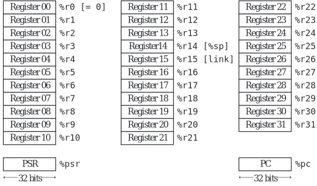
The ARC architecture contains 32 registers labeled %r0 – %r31, that each hold a 32-bit word. There is also a 32-bit Processor State Register (PSR) that describes the current state of the processor, and a 32-bit program counter (PC), that keeps track of the instruction being executed, as illustrated in Figure 4-9. The

PSR is labeled %psr and the PC register is labeled %pc. Register %r0 always contains the value 0, which cannot be changed. Registers %r14 and %r15 have additional uses as a stack pointer (%sp) and a link register, respectively, as described later.

Operands in an assembly language statement are separated by commas, and the destination operand always appears in the rightmost position in the operand field. Thus, the example shown in Figure 4-8 specifies adding registers %r1 and %r2, with the result placed in %r3. If %r0 appears in the destination operand field instead of %r3, the result is discarded. The default base for a numeric oper-and is 10, so the assembly language statement:

addcc %r1, 12, %r3

shows an operand of (12)₁₀ that will be added to %r1, with the result placed in %r3. Numbers are interpreted in base 10 unless preceded by “0x” or ending in “H”, either of which denotes a hexadecimal number. The comment field follows

Register 00 %r0 [= 0] Register 01 %r1 Register 02 %r2 Register 03 %r3 Register 04 %r4 Register 05 %r5 Register 06 %r6 Register 07 %r7 Register 08 %r8

PSR %psr PC %pc

Register 09 %r9 Register 10 %r10

Register 11 %r11 Register 12 %r12 Register 13 %r13

Register14 %r14 [%sp] Register 15 %r15 [link]

32 bits 32 bits

Register 16 %r16 Register 17 %r17 Register 18 %r18 Register 19 %r19 Register 20 %r20 Register 21 %r21

Register 22 %r22 Register 23 %r23 Register 24 %r24 Register 25 %r25 Register 26 %r26 Register 27 %r27 Register 28 %r28 Register 29 %r29 Register 30 %r30 Register 31 %r31

(16)

the operand field, and begins with an exclamation mark ‘!’ and terminates at the end of the line.

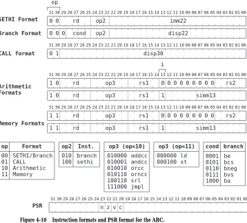
4.2.4 ARC INSTRUCTION FORMATS

The instruction format defines how the various bit fields of an instruction are laid out by the assembler, and how they are interpreted by the ARC control unit. The ARC architecture has just a few instruction formats. The five formats are: SETHI, Branch, Call, Arithmetic, and Memory, as shown in Figure 4-10. Each

instruction has a mnemonic form such as “ld,” and an opcode. A particular instruction format may have more than one opcode field, which collectively identify an instruction in one of its various forms. (Note that these four instruc-tion formats do not directly correspond to the four instrucinstruc-tion classificainstruc-tions

op3 (op=10) 010000 010001 010010 010110 100110 111000 addcc andcc orcc orncc srl jmpl 0001 0101 0110 0111 1000 cond be bcs bneg bvs ba branch 010 100 op2 branch sethi Inst. 00 01 10 11 op SETHI/Branch CALL Arithmetic Memory Format 000000 000100 ld st op3 (op=11) op

CALL format disp30

31 30 29 28 27 26 25 24 23 22 21 20 19 18 17 16 15 14 13 12 11 10 09 08 07 06 05 04 03 02 01 00

0 1

SETHI Format _imm22

31 30 29 28 27 26 25 24 23 22 21 20 19 18 17 16 15 14 13 12 11 10 09 08 07 06 05 04 03 02 01 00

rd disp22 0 cond 0 0 0 0 Branch Format op2 op2

31 30 29 28 27 26 25 24 23 22 21 20 19 18 17 16 15 14 13 12 11 10 09 08 07 06 05 04 03 02 01 00

rs1 1 op3 simm13 1 op3 1 Memory Formats 1 rd rd rs1 0 1

0 0 0 0 0 0 0 0 rs2

Arithmetic Formats

31 30 29 28 27 26 25 24 23 22 21 20 19 18 17 16 15 14 13 12 11 10 09 08 07 06 05 04 03 02 01 00

rs1 1 op3 simm13 1 op3 0 0 rd rd rs1 0 1

0 0 0 0 0 0 0 0 rs2 i

PSR

31 30 29 28 27 26 25 24 23 22 21 20 19 18 17 16 15 14 13 12 11 10 09 08 07 06 05 04 03 02 01 00

z v c n

(17)

shown in Figure 4-7.)

The leftmost two bits of each instruction form the op (opcode) field, which identifies the format. The SETHI and Branch formats both contain 00 in the op field, and so they can be considered together as the SETHI/Branch format. The actual SETHI or Branch format is determined by the bit pattern in the op2 opcode field (010 = Branch; 100 = SETHI). Bit 29 in the Branch format always contains a zero. The five-bit rd field identifies the target register for the SETHI operation.

The cond field identifies the type of branch, based on the condition code bits (n, z, v, and c) in the PSR, as indicated at the bottom of Figure 4-10. The result of executing an instruction in which the mnemonic ends with “cc” sets the condi-tion code bits such that n=1 if the result of the operation is negative; z=1 if the result is zero; v=1 if the operation causes an overflow; and c=1 if the operation produces a carry. The instructions that do not end in “cc” do not affect the con-dition codes. The imm22 and disp22 fields each hold a 22-bit constant that is used as the operand for the SETHI format (for imm22) or for calculating a dis-placement for a branch address (for disp22).

The CALL format contains only two fields: the op field, which contains the bit pattern 01, and the disp30 field, which contains a 30-bit displacement that is used in calculating the address of the called routine.

The Arithmetic (op = 10) and Memory (op = 11) formats both make use of rd fields to identify either a source register for st, or a destination register for the remaining instructions. The rs1 field identifies the first source register, and the rs2 field identifies the second source register. The op3 opcode field identi-fies the instruction according to the op3 tables shown in Figure 4-10.

(18)

The Arithmetic instructions need two source operands and a destination and, for a total of three operands. The Memory instructions only need two oper-ands: one for the address and one for the data. The remaining source operand is also used for the address, however. The operands in the rs1 and rs2 fields are added to obtain the address when i = 0. When i = 1, then the rs1 field and the simm13 field are added to obtain the address. For the first few examples we will encounter, %r0 will be used for rs2 and so only the remaining source oper-and will be specified.

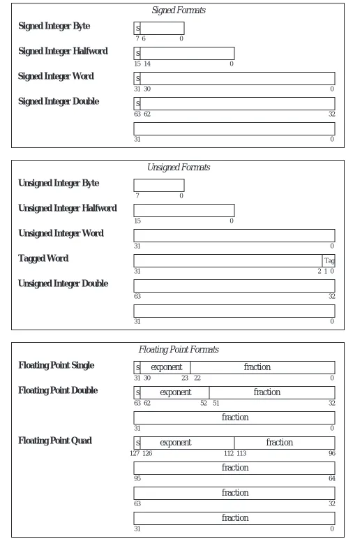
4.2.5 ARC DATA FORMATS

The ARC supports 12 different data formats as illustrated in Figure 4-11. The data formats are grouped into three types: signed integer, unsigned integer, and floating point. Within these types, allowable format widths are byte (8 bits), half-word (16 bits), half-word/singlehalf-word (32 bits), tagged half-word (32 bits, in which the two least significant bits form a tag and the most significant 30 bits form the value), doubleword (64 bits), and quadword (128 bits).

In reality, the ARC does not differentiate between unsigned and signed integers. Both are stored and manipulated as two’s complement integers. It is their inter-pretation that varies. In particular one subset of the branch instructions assumes that the value(s) being compared are signed integers, while the other subset assumes they are unsigned. Likewise, the c bit indicates unsigned integer over-flow, and the v bit, signed overflow.

The tagged word uses the two least significant bits to indicate overflow, in which an attempt is made to store a value that is larger than 30 bits into the allocated 30 bits of the 32-bit word. Tagged arithmetic operations are used in languages with dynamically typed data, such as Lisp and Smalltalk. In its generic form, a 1 in either bit of the tag field indicates an overflow situation for that word. The tags can be used to ensure proper alignment conditions (that words begin on four-byte boundaries, quadwords begin on eight-byte boundaries, etc.), particu-larly for pointers.

(19)

4.2.6 ARC INSTRUCTION DESCRIPTIONS

Now that we know the instruction formats, we can create detailed descriptions of the 15 instructions listed in Figure 4-7, which are given below. The translation to object code is provided only as a reference, and is described in detail in the next chapter. In the descriptions below, a reference to the contents of a memory loca-tion (for ld and st) is indicated by square brackets, as in “ld [x], %r1” which copies the contents of location x into %r1. A reference to the address of a

Signed Integer Byte s

7 6 0

Signed Integer Halfword s

15 14 0

Signed Integer Word s

31 30 0

Signed Integer Double s

63 62 32

31 0

Signed Formats

Unsigned Integer Byte

7 0

Unsigned Integer Halfword

15 0

Unsigned Integer Word

31 0

Unsigned Integer Double

63 32

31 0

Unsigned Formats

Floating Point Single

Floating Point Double

Floating Point Quad

31 0

s

127 126 96

95 64

Floating Point Formats Tagged Word

31 0

Tag 1 2

s

31 30 0

exponent fraction 23 22

s

63 62 32

exponent fraction

fraction

63 32

31 0

exponent fraction 52 51

113 112

fraction

(20)

memory location is specified directly, without brackets, as in “call sub_r,” which makes a call to subroutine sub_r. Only ld and st can access memory, therefore only ld and st use brackets. Registers are always referred to in terms of their contents, and never in terms of an address, and so there is no need to enclose references to registers in brackets.

Instruction: ld

Description: Load a register from main memory. The memory address must be aligned on a word boundary (that is, the address must be evenly divisible by 4). The address is computed by adding the contents of the register in the rs1 field to either the contents of the register in the rs2 field or the value in the simm13 field, as appropriate for the con-text.

Example usage: ld [x], %r1 or ld [x], %r0, %r1 or ld %r0+x, %r1

Meaning: Copy the contents of memory location x into register %r1.

Object code: 11000010000000000010100000010000 (x = 2064)

Instruction: st

Description: Store a register into main memory. The memory address must be aligned on a word boundary. The address is computed by adding the contents of the register in the rs1 field to either the contents of the register in the rs2 field or the value in the simm13 field, as appropriate for the context. The rd field of this instruction is actually used for the source register.

Example usage: st %r1, [x]

Meaning: Copy the contents of register %r1 into memory location x.

Object code: 11000010001000000010100000010000 (x = 2064)

Instruction: sethi

Description: Set the high 22 bits and zero the low 10 bits of a register. If the operand is 0 and the register is %r0, then the instruction behaves as a no-op (NOP), which means that no operation takes place.

Example usage: sethi 0x304F15, %r1

Meaning: Set the high 22 bits of %r1 to (304F15)₁₆, and set the low 10 bits to zero.

Object code: 00000011001100000100111100010101

Instruction: andcc

Description: Bitwise AND the source operands into the destination operand. The con-dition codes are set according to the result.

Example usage: andcc %r1, %r2, %r3

Meaning: Logically AND %r1 and %r2 and place the result in %r3.

(21)

Instruction: orcc

Description: Bitwise OR the source operands into the destination operand. The condi-tion codes are set according to the result.

Example usage: orcc %r1, 1, %r1

Meaning: Set the least significant bit of %r1 to 1.

Object code: 10000010100100000110000000000001

Instruction: orncc

Description: Bitwise NOR the source operands into the destination operand. The con-dition codes are set according to the result.

Example usage: orncc %r1, %r0, %r1

Meaning: Complement %r1.

Object code: 10000010101100000100000000000000

Instruction: srl

Description: Shift a register to the right by 0 – 31 bits. The vacant bit positions in the left side of the shifted register are filled with 0’s.

Example usage: srl %r1, 3, %r2

Meaning: Shift %r1 right by three bits and store in %r2. Zeros are copied into the three most significant bits of %r2.

Object code: 10000101001100000110000000000011

Instruction: addcc

Description: Add the source operands into the destination operand using two’s comple-ment arithmetic. The condition codes are set according to the result.

Example usage: addcc %r1, 5, %r1

Meaning: Add 5 to %r1.

Object code: 10000010100000000110000000000101

Instruction: call

Description: Call a subroutine and store the address of the current instruction (where the call itself is stored) in %r15, which effects a “call and link” operation. In the assem-bled code, the disp30 field in the CALL format will contain a 30-bit displacement from the address of the call instruction. The address of the next instruction to be exe-cuted is computed by adding 4×disp30 (which shifts disp30 to the high 30 bits of the 32-bit address) to the address of the current instruction. Note that disp30 can be negative.

Example usage: call sub_r

Meaning: Call a subroutine that begins at location sub_r. For the object code shown below, sub_r is 25 words (100 bytes) farther in memory than the call instruction.

Object code: 01000000000000000000000000011001

(22)

Description: Jump and link (return from subroutine). Jump to a new address and store the address of the current instruction (where the jmpl instruction is located) in the des-tination register.

Example usage: jmpl %r15 + 4, %r0

Meaning: Return from subroutine. The value of the PC for the call instruction was pre-viously saved in %r15, and so the return address should be computed for the instruction that follows the call, at %r15 + 4. The current address is discarded in %r0.

Object code: 10000001110000111110000000000100

Instruction: be

Description: If the z condition code is 1, then branch to the address computed by add-ing 4×disp22 in the Branch instruction format to the address of the current instruc-tion. If the z condition code is 0, then control is transferred to the instruction that follows be.

Example usage: be label

Meaning: Branch to label if the z condition code is 1. For the object code shown below, label is five words (20 bytes) farther in memory than the be instruction.

Object code: 00000010100000000000000000000101

Instruction: bneg

Description: If the n condition code is 1, then branch to the address computed by add-ing 4×disp22 in the Branch instruction format to the address of the current instruc-tion. If the n condition code is 0, then control is transferred to the instruction that follows bneg.

Example usage: bneg label

Meaning: Branch to label if the n condition code is 1. For the object code shown below, label is five words farther in memory than the bneg instruction.

Object code: 00001100100000000000000000000101

Instruction: bcs

Description: If the c condition code is 1, then branch to the address computed by add-ing 4×disp22 in the Branch instruction format to the address of the current instruc-tion. If the c condition code is 0, then control is transferred to the instruction that follows bcs.

Example usage: bcs label

Meaning: Branch to label if the c condition code is 1. For the object code shown below, label is five words farther in memory than the bcs instruction.

Object code: 00001010100000000000000000000101

Instruction: bvs

(23)

Example usage: bvs label

Meaning: Branch to label if the v condition code is 1. For the object code shown below, label is five words farther in memory than the bvs instruction.

Object code: 00001110100000000000000000000101

Instruction: ba

Description: Branch to the address computed by adding 4× disp22 in the Branch instruction format to the address of the current instruction.

Example usage: ba label

Meaning: Branch to label regardless of the settings of the condition codes. For the object code shown below, label is five words earlier in memory than the ba instruc-tion.

Object code: 00010000101111111111111111111011

4.3 Pseudo-Ops

In addition to the ARC instructions that are supported by the architecture, there are also pseudo-operations (pseudo-ops) that are not opcodes at all, but rather instructions to the assembler to perform some action at assembly time. A list of pseudo-ops and examples of their usages are shown in Figure 4-12. Note that

unlike processor opcodes, which are specific to a given machine, the kind and nature of the pseudo-ops are specific to a given assembler, because they are exe-cuted by the assembler itself.

The .equ pseudo-op instructs the assembler to equate a value or a character

Pseudo-Op Usage Meaning

.equ .equ #10 Treat symbol X as (10)₁₆

.begin .begin Start assembling

.end .end Stop assembling

.org .org 2048 Change location counter to 2048

.dwb .dwb 25 Reserve a block of 25 words

X

.global .global Y Y is used in another module

.extern .extern Z Z is defined in another module

.macro .macro M a, b, ...

parameters a, b, ...

.endmacro .endmacro End of macro definition

.if .if <cond> Assemble if <cond> is true

.endif .endif End of .if construct

Define macro M with formal

(24)

string with a symbol, so that the symbol can be used throughout a program as if the value or string is written in its place. The .begin and .end pseudo-ops tell the assembler when to start and stop assembling. Any statements that appear before .begin or after .end are ignored. A single program may have more than one .begin/.end pair, but there must be a .end for every .begin, and there must be at least one .begin. The use of .begin and .end are helpful in mak-ing portions of the program invisible to the assembler durmak-ing debuggmak-ing.

The .org (origin) pseudo-op causes the next instruction to be assembled with the assumption it will be placed in the specified memory location at runtime (location 2048 in Figure 4-12.) The .dwb (define word block) pseudo-op reserves a block of four-byte words, typically for an array. The location counter

(which keeps track of which instruction is being assembled by the assembler) is moved ahead of the block according to the number of words specified by the argument to .dwb multiplied by 4.

The .global and .extern pseudo-ops deal with names of variables and addresses that are defined in one assembly code module and are used in another. The .global pseudo-op makes a label available for use in other modules. The .extern pseudo-op identifies a label that is used in the local module and is defined in another module (which should be marked with a .global in that module). We will see how .global and .extern are used when linking and loading are covered in the next chapter. The .macro, .endmacro, .if, and .endif pseudo-ops are also covered in the next chapter.

4.4 Examples of Assembly Language Programs

The process of writing an assembly language program is similar to the process of writing a high-level program, except that many of the details that are abstracted away in high-level programs are made explicit in assembly language programs. In this section, we take a look at two examples of ARC assembly language programs.

Program: Add Two Integers.

(25)

only ld and st can access main memory), and so the program begins by loading registers %r1 and %r2 with x and y. The addcc instruction adds %r1 and %r2 and places the result in %r3. The st instruction then stores %r3 in memory location z. The jmpl instruction with operands %r15 + 4, %r0 causes a return to the next instruction in the calling routine, which is the operating sys-tem if this is the highest level of a user’s program as we can assume it is here. The variables x, y, and z follow the program.

In practice, the SPARC code equivalent to the ARC code shown in Figure 4-13 is not entirely correct. The ld, st, and jmpl instructions all take at least two instruction cycles to complete, and since SPARC begins a new instruction at each clock tick, these instructions need to be followed by an instruction that does not rely on their results. This property of launching a new instruction before the previous one has completed is called pipelining, and is covered in more detail in Chapter 9.

Program: Sum an Array of Integers

Now consider a more complex program that sums an array of integers. One pos-sible coding is shown in Figure 4-14. As in the previous example, the program begins and ends with a .begin/.end pair. The .org pseudo-op instructs the assembler to begin assembling so that the assembled code is loaded into memory starting at location 2048. A pseudo-operand is created for the symbol a_start which is assigned a value of 3000.

The program begins by loading the length of array a, which is given in bytes, into %r1. The program then loads the starting address of array a into %r2, and

! This programs adds two numbers

.org 2048

ld [x], %r1 ! Load x into %r1 ld [y], %r2 ! Load y into %r2 addcc %r1, %r2, %r3 ! %r3 ← %r1 + %r2

jmpl %r15 + 4, %r0 ! Return

x: 15

y: 9

.end .begin

prog1:

z: 0

st %r3, [z] ! Store %r3 into z

(26)

clears %r3 which will hold the partial sum. Register %r3 is cleared by ANDing it with %r0, which always holds the value 0. Register %r0 can be ANDed with any register for that matter, and the result will still be zero.

The label loop begins a loop that adds successive elements of array a into the partial sum (%r3) on each iteration. The loop starts by checking if the number of remaining array elements to sum (%r1) is zero. It does this by ANDing %r1 with itself, which has the side effect of setting the condition codes. We are interested in the z flag, which will be set to 1 if %r1 = 0. The remaining flags (n, v, and c) are set accordingly. The value of z is tested by making use of the be instruction. If there are no remaining array elements to sum, then the program branches to done which returns to the calling routine (which might be the operating system, if this is the top level of a user program).

If the loop is not exited after the test for %r1 = 0, then %r1 is decremented by

! %r5 – Holds an element of a .begin ! Start assembling .org 2048 ! Start program at 2048

be done ! Finished when length=0 addcc %r1, -4, %r1 ! Decrement array length

ld %r4, %r5 ! %r5 ← Memory[%r4]

addcc %r3, %r5, %r3 ! Sum new element into r3

ba loop ! Repeat loop.

done: jmpl %r15 + 4, %r0 ! Return to calling routine

length: 20 ! 5 numbers (20 bytes) in a

.org a_start ! Start of array a a: 25 ! length/4 values follow

–10 33 –5 7

.end ! Stop assembling ! %r4 – Pointer into array a ! %r3 – The partial sum

! %r2 – Starting address of array a ! Register usage: %r1 – Length of array a

! This program sums LENGTH numbers

loop: andcc %r1, %r1, %r0 ! Test # remaining elements andcc %r3, %r0, %r3 ! %r3 ← 0

ld [address],%r2 ! %r2 ← address of a ld [length], %r1 ! %r1 ← length of array a

addcc %r1, %r2, %r4 ! Address of next element a_start .equ 3000 ! Address of array a

address: a_start

(27)

the width of a word in bytes (4) by adding −4. The starting address of array a (which is stored in %r2) and the index into a (%r1) are added into %r4, which then points to a new element of a. The element pointed to by %r4 is then loaded into %r5, which is added into the partial sum (%r3). The top of the loop is then revisited as a result of the “ba loop” statement. The variable length is stored after the instructions. The five elements of array a are placed in an area of mem-ory according to the argument to the .org pseudo-op (location 3000).

Notice that there are three instructions for computing the address of the next array element, given the address of the top element in %r2, and the length of the array in bytes in %r1:

addcc %r1, -4, %r1 ! Point to next element to be added

addcc %r1, %r2, %r4 ! Add it to the base of the array

ld %r4, %r5 ! Load the next element into %r5.

This technique of computing the address of a data value as the sum of a base plus an index is so frequently used that the ARC and most other assembly languages have special “addressing modes” to accomplish it. In the case of ARC, the ld instruction address is computed as the sum of two registers or a register plus a 13-bit constant. Recall that register %r0 always contains the value zero, so by specifying %r0 which is being done implicitly in the ld line above, we are wast-ing an opportunity to have the ld instruction itself perform the address calcula-tion. A single register can hold the operand address, and we can accomplish in two instructions what takes three instructions in the example:

addcc %r1, -4, %r1 ! Point to next element to be added

ld %r1 + %r2, %r5 ! Load the next element into %r5.

Notice that we also save a register, %r4, which was used as a temporary place holder for the address.

(28)

Such was not the case when memories were orders of magnitude more expensive and CPUs were orders of magnitude smaller, as was the situation earlier in the computer age. Under those earlier conditions, for CPUs that had perhaps only a single register to hold arithmetic values, intermediate results had to be stored in memory. Machines had three-address, two-address, and one-address arith-metic instructions. By this we mean that an instruction could do aritharith-metic with 3, 2, or 1 of its operands or results in memory, as opposed to the ARC, where all arithmetic and logic operands must be in registers.

Let us consider how the C expression A = B*C + D might be evaluated by each of the three- two- and one-address instruction types. In the examples below, when referring to a variable “A,” this actually means “the operand whose address is A.” In order to calculate some performance statistics for the program fragments below we will make the following assumptions:

• Addresses and data words are 16-bits – a not uncommon size in earlier ma-chines.

• Opcodes are 8-bits in size.

• Operands and opcodes are moved to and from memory one word at a time.

We will compute both program size, in bytes, and program memory traffic with these assumptions.

Memory traffic has two components: the code itself, which must be fetched from memory to the CPU in order to be executed, and the data values—operands must be moved into the CPU in order to be operated upon, and results moved back to memory when the computation is complete. Observing these computa-tions allows us to visualize some of the trade-offs between program size and memory traffic that the various instruction classes offer.

Three-Address Instructions

In a three-address instruction, the expression A = B*C + D might be coded as:

mult B, C, A add D, A, A

(29)

operations are generic; they are not ARC instructions.) Then, add D to A (at this point in the program, A holds the temporary result of multiplying B times C) and store the result at address A. The program size is 7×2 or 14 bytes. Memory traffic is 16 + 2×(2×3) or 28 bytes.

Two Address Instructions

In a two-address instruction, one of the operands is overwritten by the result. Here, the code for the expression A = B*C + D is:

load B, A mult C, A add D, A

The program size is now 3×(3×2) or 18 bytes. Memory traffic is 18 + 2×2 + 2×2×3 or 34 bytes.

One Address, or Accumulator Instructions

A one-address instruction employs a single arithmetic register in the CPU, known as the accumulator. The accumulator typically holds one arithmetic operand, and also serves as the target for the result of an arithmetic operation. The one-address format is not in common use these days, but was more common in the early days of computing when registers were more expensive and fre-quently served multiple purposes. It serves as temporary storage for one of the operands and also for the result. The code for the expression A = B*C + D is now:

load B mult C

add D

store A

(30)

Special-Purpose Registers

In addition to the general-purpose registers and the accumulator described above, most modern architectures include other registers that are dedicated to specific purposes. Examples include

• Memory index registers: The Intel 80x86 Source Index (SI) and Destina-tion Index (DI) registers. These are used to point to the beginning or end of an array in memory. Special “string” instructions transfer a byte or a word from the starting memory location pointed to by SI to the ending memory location pointed to by DI, and then increment or decrement these registers to point to the next byte or word.

• Floating point registers: Many current-generation processors have special registers and instructions that handle floating point numbers.

• Registers to support time, and timing operations: The PowerPC 601 pro-cessor has Real-Time Clock registers that provide a high-resolution mea-sure of real time for indicating the date and the time of day. They provide a range of approximately 135 years, with a resolution of 128 ns.

• Registers in support of the operating system: most modern processors have registers to support the memory system.

• Registers that can be accessed only by “privileged instructions,” or when in “Supervisor mode.” In order to prevent accidental or malicious damage to the system, many processors have special instructions and registers that are unavailable to the ordinary user and application program. These instruc-tions and registers are used only by the operating system.

4.4.2 PERFORMANCE OF INSTRUCTION SET ARCHITECTURES

(31)

4.5 Accessing Data in Memory—Addressing Modes

Up to this point, we have seen four ways of computing the address of a value in memory: (1) a constant value, known at assembly time, (2) the contents of a reg-ister, (3) the sum of two registers, and (4) the sum of a register and a constant.

Table 4.1 gives names to these addressing modes, and shows a few others as well. Notice that the syntax of the table differs from that of the ARC. This is a com-mon, unfortunate feature of assembly languages: each one differs from the rest in its syntax conventions. The notation M[x] in the Meaning column assumes memory is an array, M, whose byte index is given by the address computation in brackets. There may seem to be a bewildering assortment of addressing modes, but each has its usage:

• Immediate addressing allows a reference to a constant that is known at as-sembly time.

• Direct addressing is used to access data items whose address is known at as-sembly time.

• Indirect addressing is used to access a pointer variable whose address is known at compile time. This addressing mode is seldom supported in mod-ern processors because it requires two memory references to access the op-erand, making it a complicated instruction. Programmers who wish to access data in this form must use two instructions, one to access the pointer and another to access the value to which it refers. This has the beneficial side effect of exposing the complexity of the addressing mode, perhaps dis-couraging its use.

Addressing Mode Syntax Meaning

Immediate #K K

Direct K M[K]

Indirect (K) M[M[K]]

Register Indirect (Rn) M[Rn]

Register Indexed (Rm + Rn) M[Rm + Rn]

Register Based (Rm + X) M[Rm + X]

Register Based Indexed (Rm + Rn + X) M[Rm + Rn + X]

(32)

• Register indirect addressing is used when the address of the operand is not known until run time. Stack operands fit this description, and are accessed by register indirect addressing, often in the form of push and pop instruc-tions that also decrement and increment the register respectively.

• Register indexed, register based, and register based indexed addressing are used to access components of arrays such as the one in Figure 4-14, and components buried beneath the top of the stack, in a data structure known as the stack frame, which is discussed in the next section.

4.6 Subroutine Linkage and Stacks

A subroutine, sometimes called a function or procedure, is a sequence of instructions that is invoked in a manner that makes it appear to be a single instruction in a high level view. When a program calls a subroutine, control is passed from the program to the subroutine, which executes a sequence of instructions and then returns to the location just past where it was called. There are a number of methods for passing arguments to and from the called routine, referred to as calling conventions. The process of passing arguments between routines is referred to as subroutine linkage.

One calling convention simply places the arguments in registers. The code in Figure 4-15 shows a program that loads two arguments into %r1 and %r2, calls

subroutine add_1, and then retrieves the result from %r3. Subroutine add_1 takes its operands from %r1 and %r2, and places the result in %r3 before return-ing via the jmpl instruction. This method is fast and simple, but it will not work if the number of arguments that are passed between the routines exceeds the number of free registers, or if subroutine calls are deeply nested.

! Calling routine

ld [x], %r1 ld [y], %r2 call add_1 st %r3, [z]

. . .

! Called routine

addcc %r1, %r2, %r3 jmpl %r15 + 4, %r0 add_1:

. . .

! %r3 ← %r1 + %r2

53 x:

10 y:

0 z:

(33)

A second calling convention creates a data link area. The address of the data link area is passed in a predetermined register to the called routine. Figure 4-16 shows

an example of this method of subroutine linkage. The .dwb pseudo-op in the calling routine sets up a data link area that is three words long, at addresses x, x+4, and x+8. The calling routine loads its two arguments into x and x+4, calls subroutine add_2, and then retrieves the result passed back from add_2 from memory location x+8. The address of data link area x is passed to add_2 in reg-ister %r5.

Note that sethi must have a constant for its source operand, and so the assem-bler recognizes the sethi construct shown for the calling routine and replaces x with its address. The srl that follows the sethi moves the address x into the least significant 22 bits of %r5, since sethi places its operand into the leftmost 22 bits of the target register. An alternative approach to loading the address of x into %r5 would be to use a storage location for the address of x, and then simply apply the ld instruction to load the address into %r5. While the latter approach is simpler, the sethi/srl approach is faster because it does not involve a time consuming access to the memory.

Subroutine add_2 reads its two operands from the data link area at locations %r5 and %r5 + 4, and places its result in the data link area at location %r5 + 8 before returning. By using a data link area, arbitrarily large blocks of data can be passed between routines without copying more than a single register during subroutine linkage. Recursion can create a burdensome bookkeeping overhead, however, since a routine that calls itself will need several data link areas. Data link areas have the advantage that their size can be unlimited, but also have the

disad-! Calling routine

st %r1, [x]

st %r2, [x+4]

sethi x, %r5

call add_2

x: ld

.dwb . . .

. . .

[x+8], %r3

3

! Called routine

ld %r5, %r8

ld %r5 + 4, %r9

addcc st

%r8, %r9, %r10 %r10, %r5 + 8 add_2:

jmpl %r15 + 4, %r0

srl %r5, 10, %r5

! Data link area

! x[2] ← x[0] + x[1]

(34)

vantage that the size of the data link area must be known at assembly time.

A third calling convention uses a stack. The general idea is that the calling rou-tine pushes all of its arguments (or pointers to arguments, if the data objects are large) onto a last-in-first-out stack. The called routine then pops the passed argu-ments from the stack, and pushes any return values onto the stack. The calling routine then retrieves the return value(s) from the stack and continues execution. A register in the CPU, known as the stack pointer, contains the address of the top of the stack. Many machines have push and pop instructions that automat-ically decrement and increment the stack pointer as data items are pushed and popped.

An advantage of using a stack is that its size grows and shrinks as needed. This supports arbitrarily deep nesting of procedure calls without having to declare the size of the stack at assembly time. An example of passing arguments using a stack is shown in Figure 4-17. Register %r14 serves as the stack pointer (%sp) which is

initialized by the operating system prior to execution of the calling routine. The calling routine places its arguments (%r1 and %r2) onto the stack by decrement-ing the stack pointer (which moves %sp to the next free word above the stack) and by storing each argument on the new top of the stack. Subroutine add_3 is called, which pops its arguments from the stack, performs an addition operation, and then stores its return value on the top of the stack before returning. The call-ing routine then retrieves its argument from the top of the stack and continues execution.

For each of the calling conventions, the call instruction is used, which saves the

! Calling routine

.equ %r14

addcc %sp, -4, %sp

st %r1, %sp

addcc %sp, -4, %sp

%sp

st call

. . .

%r2, %sp add_3

! Called routine

.equ %r14

ld %sp, %r8

addcc %sp, 4, %sp

ld %sp, %r9

addcc st

%r8, %r9, %r10 %r10, %sp %sp

jmpl %r15 + 4, %r0

add_3:

ld %sp, %r3

addcc %sp, 4, %sp

! Arguments are on stack.

! %sp[0] ← %sp[0] + %sp[4]

(35)

current PC in %r15. When a subroutine finishes execution, it needs to return to the instruction that follows the call, which is one word (four bytes) past the saved PC. Thus, the statement “jmpl %r15 + 4, %r0” completes the return. If the called routine calls another routine, however, then the value of the PC that was originally saved in %r15 will be overwritten by the nested call, which means that a correct return to the original calling routine through %r15 will no longer be possible. In order to allow nested calls and returns, the current value of %r15 (which is called the link register) should be saved on the stack, along with any other registers that need to be restored after the return.

If a register based calling convention is used, then the link register should be saved in one of the unused registers before a nested call is made. If a data link area is used, then there should be space reserved within it for the link register. If a stack scheme is used, then the link register should be saved on the stack. For each of the calling conventions, the link register and the local variables in the called routines should be saved before a nested call is made, otherwise, a nested call to the same routine will cause the local variables to be overwritten.

There are many variations to the basic calling conventions, but the stack-ori-ented approach to subroutine linkage is probably the most popular. When a stack based calling convention is used that handles nested subroutine calls, a stack frame is built that contains arguments that are passed to a called routine, the return address for the calling routine, and any local variables. A sample high level program is shown in Figure 4-18 that illustrates nested function calls. The operation that the program performs is not important, nor is the fact that the C programming language is used, but what is important is how the subroutine calls are implemented.

The behavior of the stack for this program is shown in Figure 4-19. The main program calls func_1 with arguments 1 and 2, and then calls func_2 with argument 10 before finishing execution. Function func_1 has two local vari-ables i and j that are used in computing the return value j. Function func_2 has two local variables m and n that are used in creating the arguments to pass through to func_1 before returning m.

(36)

pro-cess as routines return from their calls. The stack behavior shown in Figure 4-19 is thus produced as the result of executing compiler generated code, but the code may just as well have been written directly in assembly language.

As the main program begins execution, the stack pointer points to the top ele-ment of the system stack (Figure 4-19a). When the main routine calls func_1 at line 03 of the program shown in Figure 4-18 with arguments 1 and 2, the argu-ments are pushed onto the stack, as shown in Figure 4-19b. Control is then transferred to func_1 through a call instruction (not shown), and func_1 then saves the return address, which is in %r15 as a result of the call instruc-tion, onto the stack (Figure 4-19c). Stack space is reserved for local variables i and j of func_1 (Figure 4-19d). At this point, we have a complete stack frame for the func_1 call as shown in Figure 4-19d, which is composed of the argu-ments passed to func_1, the return address to the main routine, and the local variables for func_1.

Just prior to func_1 returning to the calling routine, it releases the stack space

/* C program showing nested subroutine calls */

00 01 02

03 04 05

06 07

08 09 10 11 12

13

14 15 16

17 18 19 20 21

Line No.

main() {

int w, z; /* Local variables */