BBN Technical Memorandum No. TM-2031
An Approximate Model for Analyzing Real-World Wireless
Network Scalability
March 26, 2012
Prepared for:
Army Research Laboratories
Prepared by:
Rayethon BBN Technologies
10 Moulton Street
Cambridge, MA 02138
Research was partially sponsored by the Army Research Laboratory and was accomplished under Cooperative Agreement Number W911NF-09-2-0053. The views and conclusions contained in this document are those of the authors and should not be interpreted as representing the official policies, either expressed or implied, of the Army Research Laboratory or the U.S. Government. The U.S. Government is authorized to reproduce and distribute reprints for Government purposes notwithstanding any copyright notation here on.
An Approximate Model for Analyzing Real-World Wireless
Network Scalability
∗Ram Ramanathan
Raytheon BBN Technologies
Abhishek Samanta
Northeastern University
Tom La Porta
Pennsylvania State University
ABSTRACT
We present a framework for non-asymptotic analysis of real-world wireless networks that captures protocol overhead, con-gestion bottlenecks, traffic heterogeneity and other real-world concerns. The framework introduces the definition of symp-totic1 scalability, and a metric called change impact value
(CIV) for comparing the impact of underlying system param-eters on network scalability. A key idea is to divide analysis into generic and specific parts connected via asignature– a set of governing parameters of a network scenario – such that analyzing a new network scenario reduces mainly to identify-ing its signature.
Using this framework, we present approximate non asymp-totic (sympasymp-totic) scalability expressions for line, mesh and clique topologies using TDMA and 802.11, for unicast and broadcast traffic, by determining the signature for each of the 12 combinations. We compare the analysis with discrete-event simulations and show that the model provides sufficiently accurate estimates of scalability. Based on the symptotic ex-pressions, we study the change impact value of underlying parameters on network scalability. We show how impact anal-ysis can be used to tune network features to meet a scaling re-quirement, and determine the regimes in which reducing rout-ing overhead impacts performance. Finally, we briefly discuss approaches for extending the symptotic framework to random and mobile networks.
1.
INTRODUCTION
Consider the following problem: a multi-hop wireless net-work running OLSR [2] routing over 802.11 radios needs to be deployed in a roughly regular structure (Manhattan grid). Each node needs a VoIP stream to another node (say randomly chosen) and is active 20% of the time. Roughly how many nodesN can one deploy?
Such a question, with straightforward variations, may arise in a deploying a wireless network in diverse situations:
de-∗
This work was partially supported by the Army Research Labora-tory and was accomplished under Cooperative Agreement Number W911NF-09-2-0053.
1
The word “symptotic” is not part of the English lexicon. Our in-spiration comes from the commentary of Euclid’s Elements by Pro-clus [1] “.. some are asymptotic, namely, those which however far extended never meet, and others that do intersect aresymptotic..”
ploying instant infrastructure after a disaster, a community mesh network in a rural area, a military infrastructure-less net-work, a sensor netnet-work, etc. Often, the answer does not need to be precise, but quick, and for a wide range of parameter combinations. Currently the only reasonable way available to answer such questions is to construct a simulation model and iterate over different values ofNto find the upper bound. Not only does this take a prohibitively long time, but also requires re-running over again to answer follow up questions: what if we used a faster radio, or used different protocols in place of OLSR and 802.11, or a different encoding for VoIP is used? What if it is a different topology or a different traffic pattern? Analytical modeling appears a natural fit. However, much of the analytical research thus far has been alongasymptotic
lines (e.g [3, 4, 5, 6]). While these have provided tremendous insight in the limiting case, asymptotic scalability has limited applicability to finite real-world networks. A network may be asymptotically unscalable, yet scale comfortably to the req-uisite number of nodes in a given deployment. For instance, a MANET with directional antennas is asymptotically unscal-able [7], but with 30 degree beamwidth can theoretically scale to about 14,000 nodes, adequate in most setting [8]. Fur-ther, such work does not consider control protocols, bottle-neck phenomena, and the multiplicity of traffic types that are an inherent part of real-world systems. While there exist some analyses of specific protocols (such as 802.11) an analytical model of anetwork scenario– a combination of the topology, protocols, node and traffic attributes – as a whole is what we need2.
In this paper, we presentsymptotics– a framework for ap-proximate non-asymptotic scalability analysis of wireless net-works. Unlike asymptotic analysis that typically characterizes a network in binary terms (does it scale or not), symptotics seeks to provide a qualified answer (how many nodes does it scale to). The framework defines the concept ofsymptotic scalability, and accommodates real-world concerns including protocol overhead effects, congestion bottlenecks and a mul-tiple traffic types such as unicast and broadcast. It provides a unified approach to analytically modeling a suite of network
2
scenarios without re-working the analysis for each, and a sys-tematic way of determining the impact of changing a scenario parameter on performance.
Our thesis is that the performance of a network scenario is dominated by a few major factors, and by focusing only on those and abstracting away all other details, one can gain rea-sonable accuracy while avoiding complexity. Specifically, we divide the model into two parts – a) a generic equation for a class of network scenarios that captures the performance in terms of a set of major factors termed thesignatureof the sce-nario; b) instantiation of this equation using the specific signa-ture of the given network scenario to derive a non-asymptotic (symptotic) expression for this network scenario. Thus, ana-lyzing a new scenario requires doing only part (b) rather than re-working from scratch. The signature-based approach con-siders the network scenario as a “whole” rather than combin-ing models for individual components.
We illustrate the application of our framework by deriv-ing approximate symptotic scalability expressions for 12 net-work scenarios resulting from combinations of three regular topologies (line, mesh, clique), two MAC protocols (TDMA, 802.11) and two traffic types (unicast, broadcast). We also outline how our framework can be extended to capture irreg-ular topologies such as random geometric networks and mo-bile networks. By virtue of the decoupling that the signature provides, each derivation reduces to identifying the signature and instantiating the generic equation and solving it to get the required expression. A comparison with simulation results show that despite their simplicity, our models are adequate for the rough estimations motivated at the beginning of this section.
A valuable part of the symptotic framework is a rigorous and uniform approach toimpact analysis, that is, which pa-rameters affect the overall system performance the most. As part of the framework, we introduce the concept of change impact value(CIV) to quantify the impact of domain param-eters in a uniform way. By comparing the CIVs, we can tell, for example, if halving the offered load is better or worse for scalability than halving the routing overhead. Impact analy-sis of even simple networks yields some interesting, counter-intuitive insights. Moreover, since impact analysis targets per-formancedifferences(for instance, before and after a parame-ter change), it is only marginally affected by the approximate nature of the model. It turns out, for instance, that the impact of routing overhead reduction on scalability is dwarfed by the impact of radio rate and load. Further, the relative impacts shift in dominance as we change the parameters of a network scenario; and contrary to intuition, routing overhead reduction in multi-hop networks is most impactful when the bandwidth to load ratio is high. Our study leads us to surmise that, while the extensive past and some ongoing work on routing over-head reduction is clever and deep, it is likely to have little practical impact in the big picture.
In the tradeoff between analytical accuracy and simplicity, our framework makes a deliberate move toward approximate,
but simpler formulations. There are two reasons for this. First, analytical characterization of a real-life system and environ-ments is inherently extremely difficult and would be near im-possible without abstractions. Second, from a pragmatic (vice pedagogical) viewpoint, an analytical model is most useful for obtaining insights into relationships and making rough order-of-magnitude analysis – the vagaries of a wireless network render even the most painstaking analysis inaccurate in prac-tice, and thus simple-but-approximate is better suited. Third, we recognize that the relationship between effort and accuracy is non-linear, and there exists a “knee” of the curve which can give us sufficient accuracy without excessive analytical effort. Our simulation validation results (detailed in section 5) bear testimony to the fact that such an approach can indeed bound inaccuracy to the desired level. Further, many analytical mod-els become so abstruse in their desire to model every single detail that they lose their ability to provide insight – the very motivation for analysis in many cases – by being too com-plicated. The symptotics framework prioritizes simplicity by ignoring those aspects modeling which will likely not yield a commensurate benefit in accuracy.
In sum, our contributions are as follows
• A new approach to scalability analysis that captures real-world aspects and enables one to roughly estimate scala-bility of a scenario by simply identifying its “signature”.
• Closed-form symptotic scalability expressions for 12 reg-ular network scenarios validated using simulations.
• A new impact analysis methodology that allows one to swiftly tune a network’s features to meet a scaling re-quirement and estimate which parameter is critical in which conditions.
The symptotics framework lays the foundation for the col-laborative development of a library of analytical models that can be incorporated into a much-needed real-world network performance prediction tool.
The rest of the paper is organized as follows. Section 3 describes the symptotic framework, and the derivation of a “master template” equation. In section 4 we illustrate the use of our framework by analyzing 12 network scenarios. In sec-tion 5 we compare the analytical model with simulasec-tion re-sults for the same network scenarios using ns-2. Impact anal-ysis is covered in section section 6. We briefly discuss imple-mentation in Sage in section 7. In section 8 we discuss how the framework can be extended beyond regular networks and in section 9 we discuss possible extensions of this work.
2.
RELATED WORK
in this area, the authors show that the per-node transport ca-pacity of arbitrary wireless networks grows asΘ(√1
n)
indi-cating asymptotic un-scalability. In [4], random mobile net-works are shown to scale asΘ(1), or in other words, asymp-totically scalable assuming unlimited delay tolerance. Di-rectional antennas are shown not to help in the asymptotic sense [7] whereas distributed MIMO [6] with some assump-tions scales asΘ(1). In this body of work, the assessment of scalability is unqualified (e.g. “Network X does not scale”), whereas symptotics seeks a qualified assessment (e.g. “Net-work X with parameter set P scales to 1000 nodes”). Further, these works do not consider real-world aspects such as proto-col effects or traffic heterogeneity.
There has been some recent work non-asymptotic analy-sis [9, 10], but these have focused on specific aspects such as spectrum sensing [9] or delay [10], or made assumptions similar to [3] and ignored protocols. Analysis of specific pro-tocols, especially 802.11, has received a lot of attention [11, 12, 13], and specific properties of OLSR [2] have been ana-lyzed [14]. Regular networks have been anaana-lyzed in [15, 16] for stability and capacity, albeit with specific focus on capac-ity regions [15] or impact of buffer sizes [16]. Related work for our impact analysis methodology is sensitivity analysis, which has been studied using simulation [17], and analytically using Automated Differentiation techniques in [18]. Some of these works consider real-world aspects, but focus on specific protocols or issues (e.g. delay) rather than the system as a whole, and are not focused on scalability.
Our work has been influenced by and borrows from several of the above works, notably [3, 12, 19, 16], and is unique in its joint consideration non-asymptotic scalability in real-world network scenarios.
3.
THE SYMPTOTIC FRAMEWORK
The fundamental entity for analysis in our framework is anetwork scenario, which we define as a particular instan-tiation of the 4-tuple: network topology (e.g. mesh, ran-dom), traffic type (e.g unicast, broadcast), node attributes (e.g. rate, number of transceivers), and control mechanisms (e.g. 802.11, OLSR).
Demand(D) Blocked(B) Residual(R)
D1 B1 D2 B2 Traffic 1
Traffic 2
A
va
il(W
)
Node m
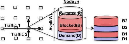
Figure 1:The different components of capacity occupation at a representa-tive node in the network.
Consider a representative node m in the network, along with its immediate neighborhood, as shown in Figure 1. We begin with a few definitions. Theavailable capacityW(m) indicates the amount of data that can be handled bym. The
demanded capacityD(m) denotes the amount of data load at
mrequired to transport a required set of flows. Theblocked capacityB(m) denotes the capacity that is unusable by node
m (for example, due to contention). Theresidual capacity R(m) is the differenceW(m) -D(m) -B(m).
We consider two main components ofB– blocking due to channel contention (Bc), and due to all other (Bo) means. As
an example of the latter consider that a node has to be quiet for a certain amount of time per second to allow sensing in a Dynamic Spectrum Access (DSA) environment.
BothDandBhave components stemming from different traffic types, each of which may have a different “cast” (uni-cast, multi(uni-cast, broadcast) and/or a different “scope” (e.g., a one hop “Hello” vs a network wide broadcast). Data, MAC control, network control, network management control etc., each have a different combination of cast and scope and are modeled as a different component ofDandB. Denoting the
jthcomponent with a subscriptjfor bothB
candBo, we have
R(m) =W(m)−X
j
Dj(m)−
X j
(Bjc(m) +Bjo(m)) (1)
In steady state, the immediate neighborhood ofmin a large network experiences approximately the same dynamics asm. Note that we do not assume thatallnodes have the same load on average. For instance, in a grid network, the center node and the corner node experience quite different loads but nodes in the neighborhood of the center (or corner) have similar loads for sufficiently large networks. Thus,
Bjc(m) = X
k∈C(m)
Dj(k) (2)
whereC(m)is the set of nodes in thecontention neighbor-hoodofmin the channel, that is, those nodes that either cause interference or in some other way causemto defer when they are active.
LetΓj(m) denote number of nodes in the contention
neigh-borhood ofm. Then, we can rewrite equation 2 as
Bj(m) = Γj(m)·Dj(m) (3)
We termΓjthecontention factorfor componentj. The
con-tention factorΓj(m)depends on the topology aroundm, on
the medium access control protocol in use, and the kind of transmission (e.g. unicast or broadcast), which in turn de-pends on the traffic typej. The contention factor is related to the spatial reuse achieved in a wireless network. The higher the contention factor, the lower is the spatial reuse.
For simplicity, letP j(m)B
o
j=Ψ(m). Thus, from
equa-tions 1 and 3, we have
R(m) =W(m)−Ψ(m)−X
j
(1 + Γj(m))Dj(m) (4)
Now considerDj(m). This is the contribution tom’s
ev-ery node sources on average the same amount of trafficLjfor
a given traffic component j. The contribution to Dj(m)is
the traffic sourced bymplus the traffic from other sources re-layed bym. We call the latter (the relayed traffic) thetransit factorofj, and denote it byΥj. For example, in a 5 node line
network with each node flooding one packet each, 4 packets are relayed by the central node, and so its transit factor is 4. A beacon signal sent periodically by a node has a transit factor of 0 since it is not relayed. The expected demanded capacity is thenDj(m)=Lj ·(1 + Υj(m)).
The loadLjfor a specific network could take into account
retransmissions, which may be different for different traffic types (esp. broadcast vs unicast)3, and additional per-data control packets (e.g. RTS/CTS/ACK per hop).
Finally, many medium access control schemes (e.g. CSMA/ CA) have non-trivialinefficiency, that is, the effective rate is lower than the actual rate. Thus, the actual capacity available for multi-access communications is a fraction ofW. Assum-ing MAC efficiency is indepenent of traffic type, and denotAssum-ing it byη, and based on the above discussion, we rewrite equa-tion 4 as
R(m) =ηW(m)−Ψ(m)−X
j
(1 + Γj(m))Lj(1 + Υj(m))
(5) A number of assumptions have been made above, notably a) contention is the only source of “blocked” capacity; b) load in a 2-hop neighborhood is roughly the same on average; and c) every node sources the same load. These assumptions al-low us to reduce the complexity of the model without com-promising on the key elements to accuracy – as evidenced by our validation results in section 5. In ongoing work not de-scribed here due to space constraints, we have relaxed (a) and are working to relax the other assumptions.
Using equation 5, we now consider the definition of symp-totic scalability and the generation of a “master template” for symptotic analysis.
From this point, the framework can be developed to derive expressions for eitherthroughput capacityfor a given set of parameters including network size orscalabilityfor a given set of parameters including loading. In this paper, we choose to focus on scalability, for several reasons. First, as motivated in the introduction, we seek to provide answers to questions such as “how many nodes will my netwroks scale to”? Sec-ond, scalability is harder to determine using simulation as it involves iterating (searching) over several network instances for “saturation”. Third, while capacity formulation is straight-forward and common, little work has been done on formal scalability formulations.
3.1
Symptotic Scalability
As motivated in section 1, we seek non-asymptotic
scala-3If we only had unicast with error rateewe could have replaceLjby,
say, Lj
1−e approximately.
bility, that is, to provide an answer to a question such as “how many nodes will my network scale to”? We begin by ob-serving that such a question only makes sense forexpandable
network scenarios, that is, those that have a “scale agnostic” specification. Examples of expandable network topologies in-cluderegulartopologies such as line, ring, mesh etc., as well asirregularstationary topologies based on some probabilis-tic model (e.g random unit-disk graphs, scale-free networks etc.), and mobile scenarios that have an expandable mobility model (e.g. the random waypoint model). An arbitrary net-work with a specific set of nodes and a specific set of links between them is not expandable because there is no “rule” to generate higher-sized versions. On the other hand, note that computing itscapacityis a reasonable proposition. A similar differentiation can be made with respect to traffic as well.
We consider the class of expandable networks for which the residual capacity monotonically decreases as the sizeN
increases. This class clearly includes regular networks with uniform traffic model. It also includes irregular expandable networks averaged over multiple instances, although a partic-ularrandom network of sizeNmay happen to have a higher residual capacity than a particular random network of size
N −1. An example of a network scenario not in this class is when the set of nodes sourcing traffic is constant (say 1). Network scenarios not in this class are arguably asymptoti-cally scalable and so are not of interest for symptotics.
For such networks, there is a point at which the monoton-ically decreasing residual capacity of an expanding network scenario transitions to negative. This is the maximum number of nodes supportable, or the “symptotic” scalability.
More precisely, letRN(m)denote the residual capacity of
nodemin a network scenario withNnodes.
DEFINITION 3.1. The symptotic scalability of a network scenario is the number of nodesXsuch that for allN ≤X, and for allm,RN(m)≥0, and for allN > X, there exists a
nodembsuch thatRN(mb)<0.
We callmbabottleneck node. Note that a network scenario
may have multiple bottlenecks, that is, nodes with equally lowest residual capacity, in which casembis any one of them.
In practice, a bottleneck node in regular networks with reg-ular traffic can be identified relatively easily for the level of accurace targeted by symptotics. For example, in a regular Manhattan grid with uniform random unicast traffic, the cen-ter node(s) are bottlnecks. If the traffic is broadcast, or the network is a mesh on a torus, all nodes are equal and every node is a bottleneck node.
With the monotonic assumption, scalability is the number of nodes at whichRis zero for the bottleneck node. Thus, the symptotic scalability of a network per the above definition can be determined by first identifying the bottleneck and applying equation 4 to that node. SettingR(mb) = 0per definition
3.1, and dropping the reference to mb with the notion that
ηW = Ψ +X
j
(1 + Γj)Lj ·(1 + Υj) (6)
whereη is the efficiency, Wis the available capacity (radio rate),Ψis the capacity not available due to reasons other than channel contention,Γjis the contention factor for traffic type
j,Ljis the average offered (sourced) load (in bps) per node
for typej, andΥjis the transit factor for trafficj.
Equation 6 may be considered the basic “master template” that we further instantiate on a per-scenario basis. This re-quires us to further expand the above parameters to generate the expression characterizing the performance for that sys-tem. Specifically, the contention factorΓjand the transit
fac-torΥjfor eachj play a critical role in the performance, and
will be referred to as the signatureof the system. To esti-mate the performance of a given system, one simply has to identify the signature and plug it into the master template. For asymptotically unscalable4 networks, the transit and/or
the contention factors are a function ofNand hence equation 6 is of the formηW =f(N, Lj), which can then be solved
forN. In section 4, we give several detailed examples of how to identify the signature of a network scenario and instantiate and solve the master template.
In contrast to previous works (e.g. those mentioned in sec-tion 2), equasec-tion 6 can capture a multiplicity of traffic types that a typical real-world system has. For instance, consider a network in which each node generates VoIP as well as web-browsing traffic, each with a different source rate and destina-tion distribudestina-tion, and addidestina-tionally a network-wide “situadestina-tional awareness” broadcast traffic. Each of these can be modeled with a separate signature (Γj,Υj). Further, control traffic is
accommodated simply as yet another traffic type.
In an system-specific instantiated expression, the Dj are
typically a function ofNand per-node sourced rate,Lj. Thus,
ifLj is given, then one can determineNas a function of the
rest of the parameters. Alternatively, ifN is given, one can determine the feasibility vector ofLj, or all but one of the
traffic typesj is given, the throughput capacity of the other can be determined.
We note that an alternate, looser definition of scalability might allow residual capacity of particular nodes to be less than zero, and require only the mean residual capacity across all nodes to be greater than zero. While our framework ac-commodates this as a branch, we do not believe real-life net-works will be operated in that regime and therefore do not consider it further.
The above applies only to networks that do not scale asymp-totically. If a network is asymptotically scalable, the residual capacity never becomes zero. Equivalently, we say that its symptotic scalability is infinity.
4
The typical multi-hop wireless network is asymptotically unscal-able [3]. While our framework can accommodate asymptotically scalable networks as well, these are largely uninteresting from a symptotic viewpoint as the scalability is infinite nodes.
3.2
Applying the Framework
Using this framework, analyzing the scalability of a real-world network scenario consists of the following steps:
For scalability, the “master template” equation 6 parame-ters are instantiated with the constants used in the system and the signature of the network – namely the contention and tran-sit factors in question. The signature can sometimes be ob-tained by simple observation, but it could also involve some non-trivial analysis, depending upon the accuracy designed. More precisely, given a network scenario, the framework can be applied using the following steps:
1. Identify the bottleneck node, if relevant. In many cases, such as regular or near-regular topologies, this is obvi-ous. In some cases, measures such asbetweenness cen-tralitycan be estimated using readily available tools. In some cases (e.g. flooded data), this is not relevant.
2. Determine the signature (Γj,Υj) for each traffic type
jfor the bottleneck node if relevant, or for an arbitrary node. Parts of the signature may be leveragable from ex-isting signatures. The signatures are typically a function of N, the number of nodes. The signature can some-times be obtained by simple observation, but it could also involve some non-trivial analysis, depending upon the accuracy desired.
3. Substitute the expressions for the signature in the “mas-ter template” equation 6 to obtain an equation in “mas-terms ofN, load (or source rates), radio rateWand other pa-rameters.
4. Solve the expression forN to get the symptotic scala-bility. Instantiate with desired values.
In the next section, we illustrate the application of the above steps for a number of network scenarios.
4.
SYMPTOTIC ANALYSIS OF NETWORK
SCENARIOS
In this section, we illustrate the application of the symptotic framework from section 3, in particular the master template equation 6, to specific network systems. Recall that a network scenario is defined as a combination of Topology, Traffic, Pro-tocol and Node models. We have analyzed systems with the following choices for each of the above aspects:
We consider 12 network scenarios generated from all pos-sible combinations of the following: three topologies –line, degree-4mesh(Manhattan grid) andclique(complete graph); two traffic types –unicastandflooding(network-wide broad-cast); and two MAC protocols –TDMA(Time Division Mul-tiple Access) and IEEE802.11DCF.
plugging it in the master equation 6, and solve forN. In sec-tion 5, we present simulasec-tion results for a subset of these sys-tems and compare with the model predictions.
In all cases, we only have one type of data traffic and two types of control traffic – routing advertizements and beacons (“Hello” broadcasts). In other words, with reference to equa-tion 6, j = 3. Thus, for the purposes of this section, the specific master equation we consider is
ηW = (1 + Γd)Ld(1 + Υd) + (1 + Γl)Ll(1 + Υl) +
(1 + Γh)Lh(1 + Υh) (7)
whereΓd,ΓlandΓhdenote the contention factors for data,
OLSR link-state updates (LSUs) and OLSR Hellos respec-tively,Υd,Υl, andΥhdenote the transit factors for data, LSUs
and Hellos respectively, andLd,LlandLhdenote the offered
load per node for each traffic type respectively.
The loadsLd,LlandLhare calculated based on the sourced
packets per second (pps) for each of data (λd), LSU frequency
(λl) and Hello frequency (λh) respectively, the payload sizes,
and the network and MAC layer headers. The header lengths and variables we use for the rest of this section are summa-rized in Table 1. To avoid too many leading or trailing zeros, all rates are in units of kbps (103bits/sec).
For network-wide broadcast (flooded) packets such as OLSR link state advertizements and flooded data, we assume a single broadcast transmission at the link layer by each node5.
We organize the rest of this section with the top level being the MAC protocol – TDMA and 802.11. For each, we illus-trate the application of the symptotic framework by analyzing the scalability of each of Line, Mesh and Clique topologies, for unicast and broadcast traffic. For each specific case, the analysis follows the steps outlined in section 3.2: a) identify the bottleneck, if relevant; b) determine the signature; c) sub-stitute the signatures in the master template to obtain the ex-pression; d) solve forN. The last step is sometimes laborious to do by hand and so we have used the Sage mathematical and symbol manipulation software [20].
The protocol parameters given in Table 1, taken from the corresponding specifications of OLSR and 802.11, are used in the remainder of this section. Note that one can keep these as “free” variables in the analysis, but instantiating them makes it easier to focus on the other parameters.
4.1
TDMA-based Regular Networks
In this section, we develop symptotic models for Line, Mesh and Clique networks with TDMA as the underlying MAC pro-tocol. Since there is no commercial standard for TDMA in multi-hop networks, we use a model based on existing litera-ture.
We consider a spatial-reuse TDMA model with node schedul-ing, also referred to a broadcast scheduling [22] and used in
5
An alternate model/assumption would be multiple unicast trans-missions at the link layer, and can also be easily analyzed with our framework if necessary.
OLSR 802.11 Variables
LSU : 52 bytes RTS : 20 bytes Data pps:λd
Hello : 48 bytes CTS : 14 bytes LSU pps:λl
Net Hdr: 20 bytes ACK : 28 bytes Hello pps:λh
MAC Hdr: 28 bytes Datarate:W
Efficiency:η
Datasize:B
Table 1:Protocol header sizes from [2, 21] and notation for free variables used in analysis.
1 2 3 1 2 3 1
B Slots
Figure 2:A conflict-free slot assignment for a line network using 3 slots.
operational systems, for example [23]. That is, time is slot-ted and slots are grouped into repeating frames. Every node is assigned a slot in a frame in which it is allowed to transmit and its neighbors receive. Thus, nodes that are neighbors or share a common neighbor should be assigned different slots. The goal of a TDMA protocol is to perform conflict-free as-signment using the least possible number of slots. Our model captures the control overhead for doing so by means of an additional “control slot” which we assume is large enough to hold any necessary messages for managing the slot assign-ment process.
Such an assignment corresponds to adistance-2 vertex col-oring problem [24, 22], that is, to color the vertices of the corresponding graph with a minimal number of colors such that nodes that are within distance-2 receive different colors. Note that node scheduling accommodates both broadcasting to neighbors as well as unicasting to neighbors.
Optimal assignment for arbitrary networks is an NP-hard problem even for planar graphs [25]. However, straightfor-ward optimal schedules are possible for the regular networks considered in this paper, and will be given in the correspond-ing sections.
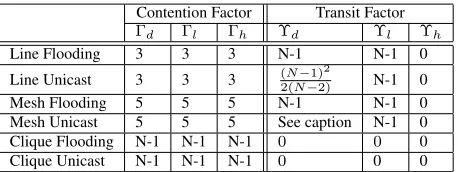
The signature set for TDMA-based networks is given in Ta-ble 2. We will refer to this taTa-ble and explain the items as we analyze each of Line, Mesh and Clique networks below.
4.1.1
Line Networks
The signature for line networks is shown in the first two rows of Table 2 and explained below.
A line network can be node scheduled using 3 slots, for example, using slot numbers 1, 2, and 3 repeating from left to right on the line (refer 2.. Thus, a typical node has to defer for nodes transmitting in other slots than its own and the control slot, and thus the contention factor is 3 for both link-layer unicast and broadcast. Since all traffic uses one of these modes, all of the contention factors are 3.
Contention Factor Transit Factor
Γd Γl Γh Υd Υl Υh
Line Flooding 3 3 3 N-1 N-1 0
Line Unicast 3 3 3 (N2(N−−1)2)2 N-1 0
Mesh Flooding 5 5 5 N-1 N-1 0
Mesh Unicast 5 5 5 See caption N-1 0
Clique Flooding N-1 N-1 N-1 0 0 0
Clique Unicast N-1 N-1 N-1 0 0 0
Table 2: Signature set for regular networks using TDMA. The transit fac-tor for data for Mesh Unicast is too long to fit in the table and is0.4(1 +
2
√
N)(N
3 4+ 4N14)
unicast flows the node at the center (two nodes ifN is even) is the bottleneck. Without loss of generality, assumeN is odd and take the center node (sayb) as the node of interest for all cases.
The TF of Hello’sΥhis clearly zero as it is single hop. The
TF for LSUsΥlis N −1 since every other node’s LSU is
transmitted by this node. Similarly, for flooded data, Υd=
N−1. For the TF of unicast data, we need to compute the ex-pected number of paths that go throughb. The probability that a given node routes throughbis the probability that the desti-nation lies on the “other side” ofb, that is,p(B)= (NN−−1)2/2. Thus, the expected number of paths isp(B)·(N−1)as shown. We now perform the next step in the symptotics approach, namely to substitute the values from the first two rows of Ta-ble 2, along with the constants from TaTa-ble 1 into equation 7. For flooding (row 1), we get
4
125(B+ 48)N λd+ 64 25N λl+
304
125λh=W η (8) Solving forN, we get the symptotic scalability of a line network running TDMA, OLSR, with network-wide broad-cast traffic as
N= 125W η−304λh
4 (Bλd+ 48λd+ 80λl)
(9)
Similarly, for unicast traffic (row 2), the equation is
2
125(N+ 1)(B+ 48)λd+ 64 25N λl+
304
125λh=W η (10) Solving for N, the symptotic scalability of a line network running TDMA, OLSR, with random unicast traffic is
N = 125W η−2Bλd−96λd−304λh
2 (Bλd+ 48λd+ 160λl)
(11)
4.1.2
Mesh Networks
We consider a mesh network ofN =mxmnodes. Such a mesh network can be scheduled using 5 slots using a straight-forward assignment scheme as shown with an example for a 7x7 mesh in Figure 3. This is tight, since there clearly is a 2-hop clique of 5 nodes each of which would need a different color. Thus, our model captures a TDMA protocol that uses 5 slots to color a mesh in addition to the control slot.
1 2 3 4 5 1 2
3 4 5 1 2 3 4
5 1 2 3 4 5 1
2 3 4 5 1 2 3
4 5 1 2 3 4 5
1 2 3 4 5 1 2
3 4 5 1 3 4 5
Figure 3:An example conflict-free slot assignment for a 7x7 mesh using 5 slots.
For network-wide broadcast (flooding), all nodes except the “border” nodes are equal bottlnecks. For unicast traffic, the node at the center (4 nodes if mis even) is the bottleneck. Without loss of generality, we assumemis odd and take the center node as the node of interest for all cases.
The signature for mesh networks is shown in Table 2 (rows 3 and 4) and explained below. Consider the contention fac-tor. With node scheduling, the node of interest has to defer for nodes transmitting in 4 slots other than its own, plus the control slot, that is, equivalent of 5 nodes. Thus, the con-tention factor is 5 in both cases for all traffic. If a sub-optimal heuristic is used, that requires, say 7 slots for scheduling the degree-4 mesh, the CF would increase correspondingly.
Consider the transit factor (TF). Clearly, the TF of Hellos is zero and that of LSAs and flooded data isN−1similar to the line. For the TF of unicast data, we need to compute the ex-pected number of paths through the center nodeb. In appendix A, we have derived an approximate formula for the number of expected paths through the center as0.4(1 + √2
N)(N
3 4 +
4N14).
Substituting the signatures for flooding and unicast from the table into the master template 7, the scalability expressions are as shown.
For flooding,
N = 125W η−456λh
6 (Bλd+ 48λd+ 80λl)
(12)
For unicast, while our estimates in section 5 are based on the derivation in Appendix A, the expression is too long to display here. We therefore give a closed-form expression us-ing a lower bound for the expected number of paths through the center as√N, derived in [16]. This lower bound also happens to correspond to the case when routing does the best possible load balancing of its traffic [16].
N = 3Bλd−
√
P+Q√3 + 144λd 2
230400λ2
l
(13)
P = 3B2λ2d+ 20000W ηλl−3840 (12λd+ 19λh)λl
Q = 96 3λ2d−10λdλl
B+ 6912λ2d
Estimates using this equation can serve as an upper bound for the performance of the considered system (since OLSR does not do load balancing).
4.1.3
Clique Networks
A clique or “complete” network is one in which all nodes are mutually adjacent. Given node scheduling, in both unicast and flooding, every packet is transmitted exactly once. Thus, the symptotics are identical for unicast and flooding.
The signature set is shown in Table 2 (last two rows). Since every node needs a slot, the CF is clearlyN−1for all three traffic types. Also, since no packet is ever relayed, the transit factors are zero for all traffic types.
No node is a bottleneck, and so any reference node can be taken. Applying the signature to 7, the symptotic scalability for both unicast and flooding is
N = 125W η
Bλd+ 48λd+ 76λh+ 80λl
(14)
4.2
802.11 based Regular Networks
In this section, we develop symptotic expressions for Line, Mesh and Clique networks with IEEE 802.11g DCF [26] as the underlying MAC protocol. As 802.11 is well known, we dispense with a summary and instead refer the reader to the Wiki page on that topic. We assume that link-level unicast transmission is always done via an RTS-CTS and DATA-ACK (RCDA) handshake, and link-level broadcast transmission con-sists simply of the DATA transmission.
In 802.11, the physical layer and MAC layer headers con-tribute to overhead that results in efficiencyη < 1. 802.11g uses OFDM and provides raw radio rates from 6 Mbps to 54 Mbps. The physical layer preamble is sent at the lowest rate and the contention window slots are fixed length. Thus, the efficiency reduces as the radio rate increases. In particular, the efficiency is roughly given by
η=
L W L W +T
(15)
whereL is the data bits, W is the rate in bps and T is the fixed overhead due to contention window, physical layer and MAC header. Based on the derivation given in [12], the datarate(W) to efficiency(η) mappings we use are: (6 Mbps
→0.80), (12 Mbps→0.70), (24 Mbps→0.58), (54 Mbps→
0.40).
We proceed to each of the topologies, applying once again the steps in the symptotic framework: a) identify the bottle-neck, if relevant; b) determine the signature (Γj,Υj) for each
j; c) substitute the signatures in the master template to obtain the expression; d) solve forN.
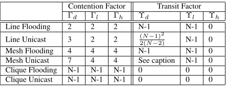
Contention Factor Transit Factor
Γd Γl Γh Υd Υl Υh
Line Flooding 2 2 2 N-1 N-1 0
Line Unicast 3 2 2 (N2(N−−1)2)2 N-1 0
Mesh Flooding 4 4 4 N-1 N-1 0
Mesh Unicast 7 4 4 See caption N-1 0
Clique Flooding N-1 N-1 N-1 0 0 0
Clique Unicast N-1 N-1 N-1 0 0 0
Table 3: Signature set for regular networks using 802.11. The transit factor for data for Mesh Unicast is too long to fit in the table and is
0.4(1 +√2
N)(N
3
4 + 4N14)
The signature set for 802.11-based networks is given in Ta-ble 3. We will refer to this taTa-ble and explain the items as we analyze each of Line, Mesh and Clique networks below. We note, however, that the transit behavior as well as the bottle-neck node is dependent on the topology and not on the MAC. Hence the transit factors are same as for the corresponding sections in the TDMA section (Table 2). Therefore, we will only discuss contention factors below, and refer the reader back to subsections in 4.1 for the explanation of the transit factor part of the signatures.
4.2.1
Line Networks
Consider the contention factor for bottleneck center node
b. For link-level unicast transmissions, without loss of gen-erality, suppose bwants to send to nodeX. Clearly, due to RTS-CTS based deference behavior,bhas to defer whenever its neighbors or neighbors ofX are transmitting, and hence the contention factor is 3. For flooded data, as well as LSAs and Hellos, since link-level broadcast is employed, RTS-CTS aren’t sent and so nodebneed only desist due to carrier sense which is when either of its neighbors are transmitting6. Hence
CF is 2.
Proceeding along the steps in the symptotic framework as done earlier, we substitute the signatures for flooding and uni-cast in master equation 7, and arrive at the expressions as fol-lows.
For flooding
N = 125W η−228λh
3 (Bλd+ 96λd+ 80λl)
(16)
For unicast
N = 2Bλd+ 125W η−192λd−228λh 2 (Bλd+ 96λd+ 120λl)
(17)
4.2.2
Mesh Networks
Consider the contention factor for bottleneck center node
b. For link-level unicast transmissions, without loss of gen-erality, supposebwants to send to nodeX. Since RTS-CTS
6
is used, all nodes that receive the RTS or the CTS defer, and by reciprocity, the reference node has a contention factor of 7. This is true for both unicast and flooding data since the latter is using multiple link-level unicasts.
For link-level broadcast transmissions (LSUs and Hellos), there is no RTS-CTS, and the only deference is via carrier sense, and hence the contention factor is all neighbors, that is, 4.
Once again, we use the lower bound on transit factor (refer section 4.1.2, and substitute the signatures for flooding and unicast in master equation 7, and arrive at the expressions as follows.
For flooding
N = 25W η−76λh
Bλd+ 96λd+ 80λl
(18)
For unicast
N = Bλd+ 96λd−
√
P+Q2
10000λ2
l
(19)
where
P = B2λ2d+ 3125W ηλl−100 (192λd+ 95λh)λl
Q = 8 24λ2d−25λdλlB+ 9216λ2d
4.2.3
Clique Networks
The signature for clique networks under 802.11 is identical to that for TDMA sinceN −1nodes cause deference by a given node.
However, there are two key factors that come into play with 802.11 that result in different symptotics. First, the over-head causes lower efficiency as discussed earlier. Second, as mentioned earlier, the backoff dynamics cause decreasing ef-ficiency with increasing numbers of nodes. That is, as the probability of collisions and finding the channel busy increase with increasing number of nodes, the efficiency of 802.11 is lower and hence a clique network with 802.11 will scale to less nodes than with TDMA. While this is negligible for fixed degree regular networks such as line and mesh, it cannot be ignored for clique as the degree isO(N). This is more thor-oughly analyzed in [19], where the efficiency is shown to de-crease asN−1.08. Using this, and the signature for 802.11
based clique as given in the last two rows, the flooding and unicast expressions are the same and is
N = 87.41
W η
Bλd+ 96λd+ 76λh+ 80λl
0.92
(20)
4.3
A Sample Instantiation
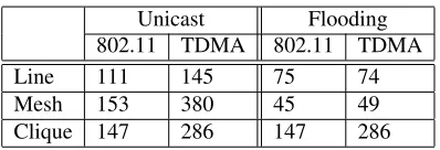
The symptotic scalability equations derived in the preced-ing sections can now be used to answer questions such as the one posed at the beginning of this paper, and variants thereof. Assume we have 1000 byte packets, and each source sends at
Unicast Flooding
802.11 TDMA 802.11 TDMA
Line 111 145 75 74
Mesh 153 380 45 49
Clique 147 286 147 286
Table 4:Scalability (maximum number of nodes) for each network scenario.
5 pps with 20% duty cycle (“on” for 20% of the time). Table 4 gives the rough order of scalability one can expect for each of the combinations, assuming OLSR at the network layer and 5 Mbps effective rate for radios.
Surprisingly, a mesh network can scale to a higher number of nodes than a line network for unicast. This is because, for unicast, mesh provides more path diversity resulting in less congestion. However for flooding this is not a factor since ev-ery node sees a packet once in both cases, and the contention in a mesh is higher. Dense networks scale the best for flooding since the number of retransmissions is low. In the next sec-tion, we present a more detailed study along with simulation results validating that the model is adequately accurate.
Apart from specific numbers, the symptotic expressions can also be used to get an insight into the dependence on parame-ters – is it linear with load (λd) or quadratic? How about with
OLSR Hello interfval (λh)? How big are the constants? A
more complete study of this follows in section 6.
5.
VALIDATION
In this section we present results of ns-2 simulations of some of the scenarios analyzed in section 4. We instantiate the corresponding symptotic expressions given there and compare them with simulation results for the same set of parameter val-ues (refer Table 1).
The TDMA protocol is an extension of the TDMA model available in the ns-2 distribution. Specifically, we have ex-tended it to a spatial reuse TDMA, that is, one that allows multiple nodes to transmit in the same slot. We then imple-mented a 3-slot assignment for line networks and a 5-slot as-signment for mesh networks as described in section 4.1. The TDMA in ns-2 already models a control slot, which we have retained.
For 802.11, we have used the ns-2 model from an overhaul that significantly improves on the original model [27]. The key features include cumulative SINR computation, pream-ble and PLCP header processing and capture, and frame body capture. The MAC accurately models the basic IEEE 802.11 CSMA/CA mechanism, as required for credible simulation studies. The model implements models of four modulation schemes – BPSK, QPSK, 16-QAM, 64-QAM – with 1/2 cod-ing rate for the first three and 3/4 for 64-QAM to provide four data rates: 6 Mbps, 12 Mbps, 24 Mbps, and 54 Mbps.
30 40 50 60 70 80 90 100 110
6000 8000 10000 12000 14000 16000 18000
Scalability
Raw data rate (kbps) Line Network, TDMA, Flooding, PPS=5
Analysis Simulation
Figure 4:TDMA, Line Network, Flooding, N vs radio rate
10 20 30 40 50 60 70 80 90 100 110
5 10 15 20 25
Scalability
Packets per second per node Line Network, TDMA, Flooding, Data Rate=18Mbps
Analysis Simulation
Figure 5: Scalability vs sourced load for flooding in a line network using TDMA, 18 Mbps radio
We have studied the symptotic scalabilityNmaxas a
func-tion of ppsλdfor each of the 12 network scenarios described
in section 4. Per definition 3.1, atN > Nmaxthe residual
ca-pacity of at least one node is less than zero. At this point, the input rate on the node’s transmit queue is more than the out-put, and the queue becomes unstable (that is, starts growing continuously). The ns-2 simulation system has a finite queue length – therefore, queue instability is detected as packets be-ing dropped due to queue bebe-ing full. Thus, we run simulations with increasing sizeNitill we encounter two consecutiveNi
andNi+1such that there are no queue drops inNi and there
are non-trivial queue drops in Ni+1. We then measure the
symptotic scalability as the average ofNiandNi+1. For
ex-ample, if there are no queue drops for N=40, and non-trivial drops for N=50, the symptotic scalability is N=45. For the line and clique networks, the increment was 10 nodes and for a mesh, the side was incremented by 1 (i.e., the sizes were 16, 25, 36, 49 and so on).
We have considered alternate measures such as a sudden drop in throughput or increase in delay. The former is fairly unreliable especially for 802.11 networks where collisons cause loss. The latter correlates well with the queue drop measure-ment, but harder to objectively measure (e.g, how much in-crease is considered “sudden”?).
Figures 4 through 11 compare the symptotic scalability
30 40 50 60 70 80 90 100 110
6000 8000 10000 12000 14000 16000 18000
Scalability
Raw data rate (kbps) Line Network, TDMA, Unicast, PPS=10
Analysis Simulation
Figure 6:TDMA, Line Network, Unicast, N vs radio rate
20 40 60 80 100 120 140 160 180 200 220
5 10 15 20 25
Scalability
Packets per second per node Line Network, TDMA, Unicast, Radio Rate=18Mbps
Analysis Simulation
Figure 7:TDMA, Line, Unicast, with 18 Mbps radio
dicted by our model with simulation results. Since the simula-tions take a long time to run for larger sizes, we picked the ra-dio rate and packets per second such that the y-axis maximum is not prohibitively large. Further, due to space constraints, we have only shown a subset of the plots, picking a subset such that each topology, MAC and traffic type is represented at least once.
Our results show that despite its simplicity and abstraction of details, the scalability predicted by our model matches that predicted by simulations fairly well, and adequately for prac-tical purposes of estimating the rough order of magnitude as motivated in section 1.
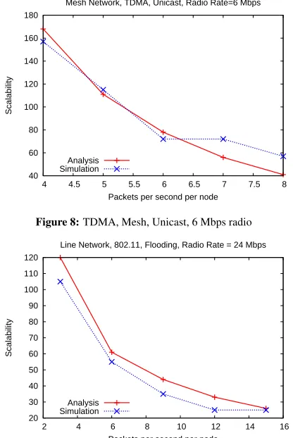
40 60 80 100 120 140 160 180
4 4.5 5 5.5 6 6.5 7 7.5 8
Scalability
Packets per second per node Mesh Network, TDMA, Unicast, Radio Rate=6 Mbps
Analysis Simulation
Figure 8:TDMA, Mesh, Unicast, 6 Mbps radio
20 30 40 50 60 70 80 90 100 110 120
2 4 6 8 10 12 14 16
Scalability
Packets per second per node
Line Network, 802.11, Flooding, Radio Rate = 24 Mbps
Analysis Simulation
Figure 9:802.11, Line, Flooding, 24 Mbps radio
N.
The simulation results attest to the fact that the approach taken and approximations and assumptions made do not ex-cessively compromise accuracy. The differences seen are within reason, and the slopes parallel for the most part. Our sim-ulation study gives us confidence that our model, despite its simplicity, is adequate for rough order of magnitude scalabil-ity predictions. In the next section, with a validated model in hand, we turn our attention to impact analysis.
6.
IMPACT ANALYSIS
In this section, we introduce a methodology for analyzing the impact of parameters such as routing overhead, radio rate, and offered load on scalability, and illustrate how it can be used to drive design choices to meet a scaling requirement. We then study how the impact changes with nominal values of network parameters.
6.1
Change Impact Value
In section 4, we derived several expressions of the form
N =f(X)whereX=(x1, x2, . . . , xn)is the parameter
vec-tor on whichN depends (see for example equation 9 in sec-tion 4).
DEFINITION 6.1. TheChange Impact FunctionCIF(xj, α)
=f(Xfxj(X=α)·xj).
10 20 30 40 50 60 70 80 90
10 15 20 25 30
Scalability
Packets per second per node Line Network, 802.11, Unicast, Data Rate = 24 Mbps
Analysis Simulation
Figure 10: Scalability vs sourced load for unicast in a line network using 802.11, 24 Mbps radio
10 20 30 40 50 60 70 80 90
5 10 15 20 25
Scalability
Packets per second per node
Clique Network, 802.11, Flooding, Radio Rate = 6 Mbps
Analysis Simulation
Figure 11:802.11, Clique, Unicast, 6 Mbps radio
The CIF expresses the effect of changing parameterxj by
a factor ofαony. The domain parameters are now elements ofXplusα.
For example, ifω =k·s2then CIF(ω,s,α) isα2. And if ω=k+s, then CIF(ω,s,α) is kk++αs·s. In the former case, the CIF is independent ofsand in the latter, it depends ons.
While the CIF is general and allows us to study the variation ofywith any subset of the parameters inX, it would be most useful to get a single value that denotes the impact of a given parameter. We do this by instantiating all variables to their nominal values.
LetVbe thenominal instantiationofX, with(x1=v1, x2=
v2, . . . , xn =vn). LetVxj=k represent that parameterxj is
instantiated with valuekinV
DEFINITION 6.2. The Change Impact ValueCIV(xj, α)
= f(Vxjf(=Vα)·vj).
In other words,CIV(xj, α)is the factor change in
scala-bility between using a particular (nominal) value for xj and
usingαtimes that value.
For example, in the expressionN=W−C, whereV = (W
= 100,C = 10),CIV(W,2)denotes the impact of doubling
The CIV depends upon the choice ofαfor the particular parameter. Increasing a parameter may increase or decrease the scalability. A parameter whose increase increases the scal-ability is calledpositively alignedand one that decreases the scalability is callednegatively aligned. To compare the im-pact uniformly, we shall chooseαp>1for positively aligned
parameters and1/αpfor negatively aligned parameters. For
instance ifαdenotes data rate,αmight be 2 and in the same analysis if xi denotes overhead, αmight be 0.5. This
de-notes, respectively, the impact of doubling the data rate or halving the overhead, and provides an apple-to-apples com-parison. The choice ofαis the users, within reasonable limits. For instance, to determine the effect of an order-of-magnitude change rather than a factor-of-2,αcould be set to 10 or 1/10 depending on the alignment. For the remainder of this section, we will useα= 2forW, andα= 0.5forλl. For brevity, we
shall often use “impact” to refer to the CIV.
A natural question is: isn’t this equivalent to simply taking the differential coefficient and evaluating/instantiating it? To see why this won’t serve our needs, consider two expressions
y = 1 +x, andy = 1000 +x, and the nominal value ofx
is 10. In both cases, dy/dx is 1, but the impact of doubling
xis much lower for the second equation (CIV=1.01) than the first (CIV=1.91), since the nominal value of the constant is much bigger in the second. The magnitude of nominal values play a crucial role in impact, and our approach is tailored to accommodate that in the simplest possible manner.
6.2
Using CIV for Network Design
We begin by illustrating how impact analysis can be used to tune a system’s features to meet a scalability requirement. Consider the following example scenario: A mesh network has to be deployed in a very remote area to provide VoIP phones, mostly for a community of about 2000 houses to talk amongst themselves. The going-in architecture is to use OLSR over 802.11b radios (max rate 11 Mbps), a G.711 VoIP codec (174 kbps duplex, 132 pps, 160 byte packets including network-layer headers) [28]. For lack of any other information, traffic is assumed to be random unicast, and we assume a conserva-tive acconserva-tive time of 20%.
Plugging these parameters into the symptotic equation 19 for 802.11-based mesh unicast in section 4, the scalability turns out to be only 116 nodes. To increase the scalability, we can either go to higher rate radios, a more efficient codec, or reduce routing overhead via a better routing protocol. We ap-ply impact analysis from section 6.1, and compute the CIVs. Usingα = 2 for radio rate (W) and α = 0.5 for source packets-per-second (λd) and routing overhead pps (λl)), we
have the CIVs as:
7
7
Technology choices offer a range of factor-of improvements, and rather than pick differentα’s for each, we have simply picked the smallest integer factor, namely 2, for simplicity. The relative CIVs forα= 2should adequately capture the relative CIVs with otherα’s for our purposes.
CIV(W) = 2.965; CIV(λd) = 2.811; CIV(λl) = 1.020
Thus, radio rate W and source rate λdare about equally
dominant, providing approximately a 3x increase in scalabil-ity. However, source rate is more easily changed by using a better codec for very little tradeoff in clarity. Suppose we pick the G.723 codec (33 kbps duplex, 66 pps, 64 byte packets) in-stead with everything else remaining the same. This is factor of 5 lower in load and therefore we should expect it to scale much more than 2.811*116 = 326 nodes. Recalculating using equation 19, the scalability is now 630 nodes, which is a vast improvement, but still well below the target 2000. Now, the CIVs are
CIV(W) = 2.588; CIV(λd) = 2.382; CIV(λl) = 1.000
Notice that depending upon the values of other nominal parameters, the impact of changing a parameter is different. In particular, the impact of changingW is now non-trivially higher. Given that we have already reduced λd, we turn to
802.11g radios with a maximum rate of 54 Mbps (a factor of ˜5 improvement). With this, the scalability is about 2507 nodes which meets the requirement. Now the CIVs are
CIV(W) = 2.502; CIV(λd) = 2.231; CIV(λl) = 1.014
This suggests that if we could further double the radio rate, we might reach 2.5*2507 = 6250 nodes.
In all of the above, we notice that the CIV(λl), that is,
the impact of routing load is negligible. Specifically, for the above realistic scenario, halving the routing overhead will pro-vide a mere 1.014x increase in scalability, far below the im-pact of the other parameters. While it is not surprising that radio rate and load are more impactful, we were surprised by themagnitudeof the difference.
What if we replace 802.11 by TDMA – although TDMA is not readily commercially available in WiFi cards, it can be implemented as an overlay [29], and in any case, it would be interesting to know. Replacing 802.11 by TDMA in our framework simply requires replacing with a different signa-ture, specifically, the one in Table 2. Keeping the 54 Mbps raw rate and G723.1 codec, the scalability turns out to be a 16230 nodes! The CIVs now interestingly, are not so asym-metric
CIV(W) = 2.360; CIV(λd) = 1.778; CIV(λl) = 1.171
6.3
A Study of Impact
1 1.01 1.02 1.03 1.04 1.05 1.06 1.07 1.08
1 2 3 4 5 6 7 8 9
CIV LSU pps
Packets per second per node Line Network, TDMA, Rate=22 Mbps
Flooding Unicast
Figure 12:Impact of reducing routing overhead on scalability as a function of load for flooding and unicast in a line network.
1 1.5 2 2.5 3 3.5 4
1 2 3 4 5 6 7 8 9 10
Change Impact Value (CIV)
Packets per second per node 802.11, Mesh, Unicast, Radio Rate=54 Mbps
CIV Rate CIV Load CIV Routing
Figure 13:Comparing the impact of changing radio rate, source load and overhead on scalability (higher CIV means more impactful)
by a factor of 2 (ie,α= 2 or 0.5).
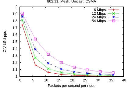
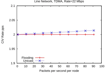
Figure 12 shows that the impact of overhead reduction on scalability is higher for lighter load. This is because at lower loads LSUs are allowed to occupy a higher fraction of the capacity, and therefore has more impact when changed. For the same reason, impact is lower for flooding traffic which imposes a higher overall network load for the same sourced load
Figure 13 shows the CIVs of radio rate, source load and overhead over a range of traffic loads. For a vast majority of this space, the impact of doubling radio rate or halving source load is vastly higher than halving overhead. The gap narrows at very low loads where reducing overhead becomes about equally important as halving offered load. This is because at low loads, the network scales to larger sizes in which routing overhead (which grows asO(N)per node) occupies a larger fraction of the capacity. On the other hand, this is the regime in which scalability is at its highest, and one may not need the increase quite as much as at higher loads.
Figure 14 shows that the impact of overhead reduction is much higher for a regular mesh than for line or clique, and higher when load balancing is used. This is because the lower the effective load on the bottleneck, higher is the fraction of LSUs, and consequently more impactful it is.
1 1.1 1.2 1.3 1.4 1.5 1.6 1.7 1.8 1.9
1 2 3 4 5 6 7 8 9
CIV LSU pps
Packets per second per node 802.11, Radio Rate=54 Mbps, Unicast
Line Mesh-LB Clique Mesh-NoLB
Figure 14:Impact of reducing routing overhead on scalability as a function of load for line, clique and mesh topologies (higher CIV means more impact-ful).
1 1.1 1.2 1.3 1.4 1.5 1.6 1.7 1.8 1.9 2
0 5 10 15 20 25 30 35 40
CIV LSU pps
Packets per second per node 802.11, Mesh, Unicast, CSMA
6 Mbps 12 Mbps 24 Mbps 54 Mbps
Figure 15:Impact of halving routing overhead on scalability as a function of load for different data rates
Figures 15 and 16 shows that the impact increases with in-creasing radio rate or dein-creasing data load in a mesh. Al-though not shown, the behavior is similar for other topologies. Again, this is due to the fact that the overhead component of a node’s capacity is higher at larger rate-to-pps ratios and there-fore reducing the overhead by a factor of 2 frees up relatively more capacity. Note that this is a consequence of the data be-ing unicast and the LSUs bebe-ing flooded, and so asN grows commensurate with increasing rate-to-pps ratio, LSU occu-pancy grows faster relative to data occuoccu-pancy.
1 1.1 1.2 1.3 1.4 1.5 1.6 1.7 1.8 1.9 2
5 10 15 20 25 30 35 40 45 50 55
CIV LSU pps
Radio rate (Mbps) 802.11, Mesh, Unicast
1 pps 6 pps 11 pps 16 pps
Figure 16:Impact of reducing routing overhead on scalability as a function of radio rate for a mesh network with load-balanced unicast forwarding.
1.9 1.95 2 2.05 2.1
0 10 20 30 40 50 60 70 80 90 100
CIV Rate pps
Packets per second per node Line Network, TDMA, Rate=22 Mbps
Flooding Unicast
Figure 17: Impact of radio rate increase on scalability for line unicast and flooding.
dio rate and data load. Figures 17, and 18 show CIV of radio rate and figure 19 shows the CIV of load. The observed rela-tionships can be explained similar to explanations above. At some point though, it is best to simply refer to the the corre-sponding Change Impact Functions (CIFs) for insight. Here is where having a closed form symptotic expression helps. For instance, Figure 17 can be understood from the correspond-ing equations (see section 4) whereNis seen linear toW and hence impact is roughly proportional toαwhich is 2.
We have gained a number of insights from impact analy-sis. First, as we have shown, computing the CIVs can assist in deciding which of several options provides the designer the most benefit for a given cost. Second, it appears that for most network scenarios the impact of radio rate and load on scal-ability is far higher than that of control overhead. Further, the absolute value of CIV for typical networks is close to 1, which means reducing it is largely ineffective for scalability8
While it increases with increase in radio rate or decrease in load, these network scenarios are precisely those in which we are likely not hurting for scalability. Third, topologies with more opportunities to spread out traffic (e.g. mesh with
uni-8
Although our impact analysis has not considered mobile networks, we have used an LSU source rate of 0.2 LSUs per second which captures mobilities with link dyanmics of up to once every 5 seconds.
2 2.5 3 3.5 4 4.5
0 10 20 30 40 50 60 70 80 90 100
CIV Rate
Packets per second per node TDMA, Unicast, Rate=22 Mbps
Line Mesh-LB Clique Mesh-NoLB
Figure 18:Impact of radio rate increase on scalability for various topologies as a function of load.
1.5 2 2.5 3 3.5 4 4.5
5 10 15 20 25 30 35 40 45 50
CIV Data PPS
Rate TDMA, Unicast, PPS=66
Line Mesh-LB Clique Mesh-NoLB
Figure 19:Impact of offered load decrease on scalability for various topolo-gies as a function of radio rate.
cast) offer more gain from reducing overhead, reducing load or increasing radio rate. In particular, load balancing can sig-nificantly amplify the impact of routing protocol efficiency gains.
In the past, much emphasis has been placed on ideas for reducing routing overhead. In the big picture, though, im-proving the radio rate and codec technologies is much more impactful than overhead reduction in real-life wireless net-works. On the other hand, load balancing has received scant attention relatively and holds the potential, in certain network scenarios for better impact.
7.
IMPLEMENTATION
The analytical model presented thus far in this paper has been implemented within the Sage mathematical software [20]. Sage is a free open-source mathematics software system li-censed under the GPL. It combines the power of many ex-isting open-source packages into a common Python-based in-terface. Its mission is to “create a viable free open source alternative to Magma, Maple, Mathematica and Matlab”.
simple as this
GenEqn = (1+gd)*Ld*(1+Sd) + (1+gl)*Ll*(1+Sl) + (1+gh)*Lh*(1+Sh) == W*eta
GenSoln = solve(GenEqn,N) show(GenSoln)
The (gd, gl and gh) are the contention factors for data, LSU and Hello respectively. The (Sd, Sl, Sh) are the corresponding transit factors9. These are initialized (in some cases as a
func-tion of N) prior to this block (not shown). We have coded the signatures (contention and transit factors) presented in Tables 2 and 3 into Sage.
Running any of the network scenarios consists simply of initializing the parameters in the following block to the ap-propriate value.
# Scenario Definition
macProt = ’TDMA’ # options CSMA, TDMA
topology = ’mesh’ # options line, clique, mesh
cast = ’unicast’ # options unicast, flooding
loadBalance = ’No’ # only affects mesh unicast, options Yes/No
The Change Impact Functions and Change Impact Value for LSU load, data load and radio rate are also coded in Sage, thus allowing compuation of CIVs as given in the plots in section 6.
Although Sage provides plotting as well, we have used Gnu-plot for Gnu-plotting since the latter allows us to also include the simulation results for comparison, as presented in section 5.
Finally, Sage has a facility by which a worksheet can be shared with other collaborators so that it can be edited by any of the collaborators. One may also publish a worksheet so that anybody can experiment with changing parameter values.
8.
IRREGULAR TOPOLOGIES
The symptotic scalability and impact analysis in preced-ing sections have focused on regular topologies, such as line, clique and mesh. What if the network is not regular, or is mo-bile? Can the framework accommodate irregular topologies? We briefly discuss, as space permits, some approaches that we are pursuing in this regard.
First, recall from section 3 that the notion symptotic scal-ability is reasonable only for expandablescenarios, that is, those that have a “scale agnostic” specification that can be used at any size. Examples of irregular expandable network topologies include random geometric graph [30], mobility us-ing random waypoint model, power-law degree distributed network, etc10. We consider random geometric graphs, which
have been extensively used for analyzing multi-hop networks.
9
The command in the third line above displays the answer, including in latex form, which can then be used in a manuscript. Indeed, all of the expressions given in section 4 were output from Sage.
10
We note that the residual capacity may not be monotonic with size in specific random network instances at each size, however, the av-erage over large samples at each size should be.
In this model, nodes are assumed to have a transmission range
rand are placed in a plane with theirxandycoordinates cho-sen uniformly at random. A link exists between two nodes iff their Euclidean distance is less than or equal to r. Random geometric graphs can be created at any desired density by ap-propriately adjusting the area of the plane.
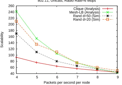
A simple, practical approach is to not analyze a random geometric network directly, but use the analysis of regular networks as a proxy. For example, a mesh network and a clique network may reasonably be considered extreme prox-ies of sparse and dense random geometric networks respec-tively. Perhaps the mesh and clique may simply “bound” the scalability of a random network? To test out this idea, we sim-ulated random geometric networks in ns-2 using 802.11 with random unicast traffic with the same parameters as in section 5, and compared with the analytical estimates of mesh and clique networks representing two extremes of density. Our results are shown in Figure 20. The simulated scalability of the random networks lies in-between the analytical estimates of the load-balanced mesh and clique for most points in the range, with fairly tight bounds at higher loads. Further, the sparser of the two random networks (density 20 nodes/sq km) tracks closer to the performance of the mesh, and the denser random network (density 50 nodes/sq km) to clique, as would be expected. In practice, establishing such bounds may be sufficient for the kinds of problems motivated in section 1, es-pecially if more regular networks are used (e.g. a degree-8 mesh).
The above approach, however, does not provide closed-form expressions for the random network, and therefore does not enable impact analysis. Symptotic analysis of a random network requires thesignature(contention and transit factors) of the random network need to be obtained. For a random network, the contention factor of a node is captured by its de-gree, and the degree of its neighbors. The bottleneck node, which is needed only for unicast, is related to the notion of
centrality. Specifically, the bottleneck node is one that has the highest betweenness centrality [31]. The betweenness cen-trality multiplied by(N−1)also yields the transit factor. A number of tools stemming from social network analysis [32] can be leveraged to compute such measures and create the sig-nature for random networks. Another approach is to use the theory of random graphs to arrive at the transit factor (i.e., the stochastic equivalent of the analysis in Appendix A).
40 60 80 100 120 140 160 180 200 220 240 260
4 5 6 7 8 9
Scalability
Packets per second per node 802.11, Unicast, Radio Rate=6 Mbps
Clique (Analysis) Mesh-LB (Analysis) Rand d=50 (Sim) Rand d=20 (Sim)
Figure 20: Comparing simulated random geometric networks of varying densitiesdwith analytical estimates of clique and mesh.
factor and transit factors over time need to be computed. Fur-ther, if the routing protocol is subject to “event driven” up-dates, then the control overhead is a function of the mobility parameters (e.g. random waypoint parameters). The idea of using stationary regular networks to bound the performance is applicable to a mobile scenario as well, but we have not performed any experiments.
Clearly, much work needs to be done for irregular expand-able networks, but we believe that the key elements of the symptotics framework – scalability concept, signature identi-fication, master template, change impact value – are still valid, and can be extended to accommodate irregular networks.
9.
DISCUSSION
In this section, we discuss some benefits, shortcomings and extensions of the symptotics framework and its application.
The general methodology we have used to analyze the 12 network scenarios can be applied to a number of other sce-narios as well. Such network scesce-narios include different node constraints such as multi-channel, multi-radio networks [33], other MAC protocols such as busy-tone [34], traffic patterns (non-random unicast, multicast, sensor sink), and topologies (8-degree grid, ring). Each of these results is a new signa-ture which can be plugged into the master template and using a tool such as Sage have an expression and actual scalability and change impact values in a matter of minutes.
Although the framework was presented with an emphasis on scalability, that is, withN being on the left hand side of equations, it is equally valid to estimate the capacity (max-imum possible throughput) as a function ofN. To do this, we simply have to solve forλd rather thanN in the specific
symptotic expression (e.g. in the equation 9). A study of the throughput capacity for the 12 network scenarios and the as-sociated impact analysis is again fairly easily done.
For now, we have deliberately chosen regular networks that span the range from extreme sparseness to extreme denseness. As briefly discussed in section 8, we beli
![Table 1: Protocol header sizes from [2, 21] and notation for free variablesused in analysis.](https://thumb-us.123doks.com/thumbv2/123dok_us/586476.2057869/7.612.337.531.177.209/table-protocol-header-sizes-notation-free-variablesused-analysis.webp)