University of Mazandaran, Iran
http://cjms.journals.umz.ac.ir
ISSN: 1735-0611
CJMS.8(1)(2019), 1-9
RBF-Chebychev direct method for solving variational problems
Ahmad Golbabai 1 and Ahmad Saeedi2
1,2 Department of Mathematics, Iran University of Science and Technology, Narmak, Tehran, Iran
Abstract. This paper establishes a direct method for solving variational prob-lems via a set of Radial basis functions (RBFs) with Gauss-Chebyshev collocation centers. The method consist of reducing a variational problem into a mathemati-cal programming problem. The authors use some optimization techniques to solve the reduced problem. Accuracy and stability of the multiquadric, Gaussian and inverse multiquadric RBF is examined and compared by some numerical experi-ments.
Keywords: Radial basis functions direct method variational problems -Gauss-Chebyshev centers.
2000 Mathematics subject classification: 49M37, Secondary 49M05.
1. Introduction
The calculus of variations investigates methods that permit maximal or minimal values of functionals[6]. Functional minimization problems naturally occur in engi-neering, mechanics, economics and so forth where minimization of functionals such as Lagrangian, potential and total energy, etc. give the laws governing the system behavior[1].
A direct method converts the variational problem into a mathematical program-ming problem. The idea of direct methods for solving variational problems consists in replacing the problem of searching for the extremum (usually, for the point of stationary) of a functional in the function space by a problem of searching for a
1Corresponding author: [email protected] Received: 10 December 2013
Revised: 8 February 2015 Accepted: 10 September 2015
Table 1. Some popular RBFs.
Name ϕ(r, c)
Gaussian (GA) ϕ(r) =exp(−cr2)
Multiquadric (MQ) ϕ(r) =√c2+r2
Inverse multiquadric (IMQ) ϕ(r) = (c2+r2)−1/2
solution in a finite set of parameters. The Ritz method [8] usually based on the sub-spaces of kinematically admissible complete functions, is the most commonly used approach in direct methods for solving variational problems.
In the last decades , Radial Basis Functios (RBFs) have been widely applied in different fields such as multivariate function interpolation and approximation, neural networks and solution of differential and integral equations. The essence of RBF interpolation is to use linear combination of ϕ(∥x−xj∥) , which is radially symmetric about its centerxj to approximate the unknown functiony(x). Common choices for RBFs are listed in Table 1 where r = ∥x −xj∥ and ∥.∥ denotes the Euclidean norm, andxjsare the centers of RBFs andcis a positive shape parameter which controls the flatness (width) of the basis function.
Franke and Schaback [7] used RBFs for solving PDEs , Golbabai and Seifollahi [10] used RBFs for solving the second kind integral equations (IEs). Moreover, it has been observed that certain class of RBFs such as multiqudric (MQ) and Gaussian(GA) RBFs exhibit superior error convergence properties [19] , [20]. Some advantages of the RBF-Based methods are their ease of implementation , accuracy and efficiency , which are the reasons that this technique is getting popular.
2. Main Results
Approximation of a functiony(x) may be expanded as
y(x)∼=yN(x) = N ∑
i=0
aiφ(∥x−xi∥), (2.1)
where N is the number of RBFs and ais are the unknown coefficients and xi are the Gauss-Chebyshev centers.
proposition 1. Let yN(x) = aTϕ(x) where aT = [a1, a2, ...aN] and ϕ(x) = [φ1(x), ..., φN(x)]T , ϕi(x) = (c2+∥x−xi∥2)
−1
2 for i = 1, ..., N. Then there exist symmetric matricesAIM Q, LIM Q and vectorϕ(x) such that:
a) (yN(x))2=aTAIM Qa, (2.2)
whereAIM Qij =φi(x)φj(x).
b) d
dxy
N(x) =aTϕ(x), (2.3)
whereϕ(x) = [φ1(x), ..., φN(x)]T and φi(x) =−(x−xi)(c2+∥x−xi∥2)
−3 2 .
c) ( d
dxy
N(x))2 =aTL
IM Qa, (2.4)
whereLIM Qij = (x−xi)(x−xj)(c2+∥x−xi∥2)
−3
2 (c2+∥x−xj∥2)− 3 2 . Proof.
The properties can be verified by the fact that ifa, b∈RN then one can see that (aTb)2 =aTb(aTb) =aTbbTa=aTA, whereAij =bibj is a symmetric matrix.
Similar properties can be verified for MQ and GA RBFs.
2.1. RBF-Chebyshev direct method. Consider the problem of finding the ex-tremum of the functional
min ∫ xb
xa
L(x, y,y˙)dx, (2.5)
where y : [xa , xb]→ RN is a suffiecitly smooth function, y(xa) = A, y(xb) = B which two points A and B inRN are given.
Tonelli’s theorem [4] says under assumptions
(1) Coercivity of rank r >1 for certain constants α >0 andβ we have
L(t, x, v)≥α∥v∥r+β. f or every (t, x, v)ϵ[a , b]×RN ×RN
(2) Convexity: Lvv is everywhere positive semidefinite (Lvv ≥0),
Euler-Lagrange equation leading to a necessary condition for y(x) on extremizing
J(y) in the form of the well known Euler-Lagrange equation
∂L ∂y −
d dx(
∂L
∂y˙) = 0, (2.6)
which can be easily solved only in a few classes. Thus it is more practical to use numerical and direct methods such as the Ritz method.
Using a Gauss-Legendre quadrature with mnodes for integrating yields:
∫ xb
xa
L(x, y,y˙)dx∼= xb−xa 2
m ∑
k=1
wkL(xk, aTϕ(∥xk−xi∥), aT
dϕ
dx(∥xk−xi∥)) (2.7)
wherexk= xb+2xa+xb−2xazk,zksandwksfork= 1, ..., mare nodes and coefficients of Gauss-Legendre quadrature and RBF centersxi, i= 1, ...N are Chebyshev nodes. Finally the variational problem (2.5) will be reduced to a constrained optimization problem of finding
minJ(a) = xb−xa 2
m ∑
k=1
wkL(xk, aTϕ(∥xk−xi)∥, aT
dϕ
dx(∥xk−xi∥)), (2.8)
subject to
aTϕ(∥xa−xi∥) =A, aTϕ(∥xb−xi∥) =B. (2.9)
To solve the optimization problem (2.8)-(2.9) our choice is to use Lagrange multi-pliers method , so we establish Lagrangian
J∗(a) =J(a) +λ1(aTϕ(∥xa−xi∥)−A) +λ2(aTϕ(∥xb−xi∥)−B), (2.10)
then we should solve the following algebraic system in order to calculate coefficients
aT = [a0, a1, ..., aN]
∂J∗
∂a = 0, (2.11)
∂J∗ ∂λi
= 0 i= 1,2. (2.12)
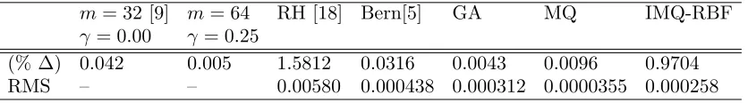
Table 2. results of example 1.
m= 32 [9] m= 64 RH [18] Bern[5] GA MQ IMQ-RBF
γ = 0.00 γ = 0.25
(% ∆) 0.042 0.005 1.5812 0.0316 0.0043 0.0096 0.9704 RMS – – 0.00580 0.000438 0.000312 0.0000355 0.000258
2.2. Solving by BiCGSTAB. For solving a general linear system two different classes are available: first, direct methods, including gaussian elimination and its variants such as LU, Cholskey. Second, iterative methods such as bicg, bicgstab, gmres, lsqr.
Sometimes solving the linear systems by a direct routin such aslinsolvein MAT-LAB returns a warning:”Matrix is close to singular or badly scaled, Results may be inaccurate”, so there is warning that the results may be unreliable. To avoid this warning we suggest to use an iterative routin such as bicgstab to solve the system.
the biconjugate gradient stabilized method (BiCGSTAB) is an iterative method. It is a variant of the BiCG (biconjugate gradient method) and has faster and smoother convergence than the original BiCG as well as other variants such as the CGS (conjugate gradient square method)
2.3. Chebyshev nodes. The Chebychev nodes are important in approximation theory because they form a particularly good set of nodes for polynomial interpo-lation. For a given natural n, chebyshev nodes in the interval [−1, 1] are xk =
cos(2k2−n1π), k = 1, ..., n. These are the roots of the chebychev polynomial of the first kind of degreen. For nodes over an arbitrary interval [a, b] an affine transform can be used
xk=
xb+xa
2 +
xb−xa 2 cos(
2k−1
2n π), k= 1, . . . , n. (2.13)
3. Examples
Example 3.1. [18], [9], [5] Find the extremal of the following functional
J(y) =
∫ 1
0
y′2(x) +xy′(x) +y(x)2dx. (3.1)
The boundary conditions are
y(0) = 0 , y(1) = 1
4. (3.2)
The exact solution of the problem is y∗(x) = 12 +c1ex +c2e−x , c1 = 4(2e−2−e1) ,
c2 = e−2e 2 4(e2−1) .
Figure 1. a) exact solution b) Absolute error vs. variable x for some RBFs.
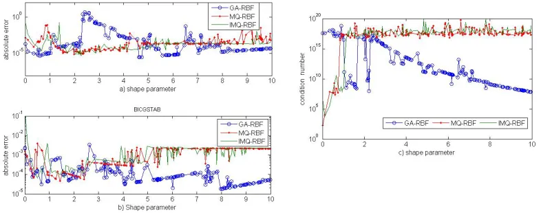
Figure 2. a) Absolute error vs. shape parameter. b)Absolute error when Using Bicgstab method. c) Condition number vs. shape parameter.
problem (3.1)-(3.2) will be reduced to an (N+ 2)×(N+ 2) algebraic linear system can be solved via MATLAB software.
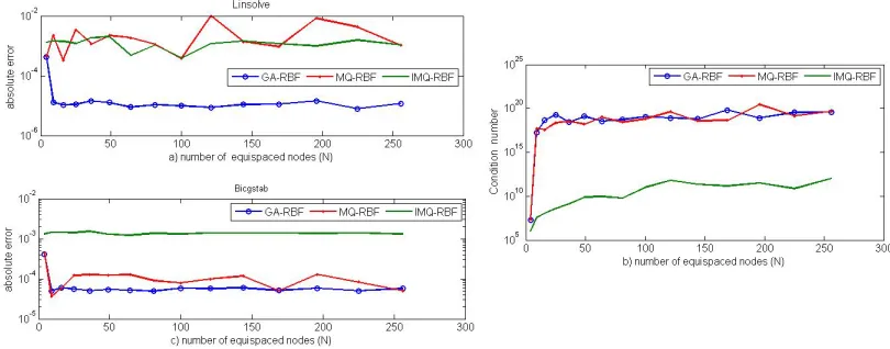
Figure 3. a) Absolute error vs. Number of equispaced nodes(N) . b) Condition number vs. number of equispaced nodes(N). c) Absolute error when solving by BiCGSTAB
Relative error△(%) for approximate solutions obtained here defined as:
∆(%) = m∑−1
j=0
∥yje−yaj∥2
m∑−1
j=0
∥yje∥2×100% (3.3)
where yej and yja denote values of state y at the jth center point of the analysed interval for respectively the exact solution and the approximate solution for different approximation degreesmand different values of parameterγand different RBF bass (GA, MQ and IMQ) withN = 36 chebyshev center points.
The formula for the root mean square errorRM Serror is given by
RM Serror = v u u t 1
M
M ∑
j=1
∥yej−yaj∥2 (3.4)
whereM is the number of selected test nodes and yej, yja are as previous.
Figure 2 (a ,b) compares absolute error of GA, MQ and IMQ RBFs for various random shape parameteres between 0 and 10. It is obvious from the figure that solving the system by command linsolve makes the results more fluctuating than when solved by BiCGSTAB.
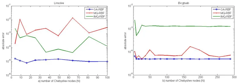
Figure 4. a) Absolute error vs. Number of chebyshev nodes(N) . b) Absolute error when solving by BiCGSTAB.
Roundoff error is a fundamental part of any numerical computation. Numerically stable methods attempt to control roundoff error and stop it from accumulating too quickly. Figures 3 , 4 demonstrates that increasing number of equally/Chebyshev spaced nodes does not yield uncontrolled increase in error, so it can be inferred that the proposed method is numerically stable. There is not significant difference in behaviour of solution in GA-RBF and MQ-RBF cases.
4. Conclusion
In this paper some properties of RBFs including IMQ-RBF were considered. Then a method that reduces the variational problem to a constrained optimization problem was described.
Numerically with the RMS and relative error criterias, it was proved that GA-RBF and MQ-GA-RBF method accuracy is better than RH and Bernstein method.
The reduced linear algebraic system was proposed to solve by some kind of pre-conditioner including BICGSTAB that enhances the reliability of the results so there is no more WARNING from MATLAB to solve the corresponding linear system. To improve the efficiency of the method, Chebyshev nodes were used as center points of RBFs. Finally numerical stability of the method was examined and verified by some numerical experiments.
References
[1] Om P. Agrawal,Formulation of Euler-Lagrange equations for fractional variational problems. J. Math. Anal. Appl. 272 (2002) pp. 368-379.
[3] C. F. Chen , C. H. Hsiao ,A walsh series direct method for solving variational problems, Journal of the Franklin Institue, 300 (1975) pp. 265-1373.
[4] Clarke, F., Functional Analysis, Calculus of Variations and Optimal Control, Springer, (2013). [5] S. Dixit, V. K. Singh, A. K. Singh, O. P. Singh,Bernstein Direct Method for Solving Variational
Problems, International Mathematical Forum, 5(2010), 2351 - 2370.
[6] L. Elsgolts ,Differentiarl equations and Calculus of Variations, Mir, Moscow. 1977 ,translated from the Russian by G. Yankovsky.
[7] C. Franke , R. Shaback,Solving Partial Differential Equations by collocation using Radial Basis Dunctions, Applied Mathematics and Computation, Volume 93, Issue 1 (1998) , pp. 73-82. [8] I. M. Gelfand, S.V. Fomin,Calculus of Variations, Prentice Hall, Englewood cliffs, NJ, 1963. [9] W. Glabisz,Direct walsh-wavelet packet method for variational problems, Applied Mathematics
and Computation , 159 (2004), pp. 769-781.
[10] A. Golbabai , S. Seifollahi, Numerical Solution of the Second kind Integral Equations using Radial Basis Functions networks, Applied Mathematics and Computation, 174 (2006), pp. 877-883.
[11] I.R. Horng, J. H. Chou,Shifted Chebyshev direct method for solving variational problems, In-ternational Journal of systems science , 16 (1985) , pp. 855-861.
[12] C. H. Hsio, Haar wavelet direct method for solving variational problems, Mathematics and Computers in Simulation, 64 (2004), pp. 569-585.
[13] C. Hwang, Y.P. Shih ,Optimal control of delay systems via block-pulse functions, Journal of optimization theory and applications, (1985) pp. 101-112.
[14] C. Hwang , Y. P. Shih , Laguerre series direct method for variational problems, Journal of optimization theory and applications, (1983) pp. 143-149.
[15] M. Maleki and M. Mashali-Firouzi,A numerical solution of problems in calculus of variation using direct method and nonclassical parametrization,J. of Computational and Applied MAth-ematics., 234 (2010), pp. 1364-1373.
[16] M. Razzaghi and S. Yousefi,Legendre wavelets direct method for variational problems, Mathe-matics and Computers in Simulation, 53 (2000), pp. 185-192.
[17] M. Razzaghi , S. Yousefi ,Sine-Cosine wavelets operational matrix of integration and its appli-cations in the calculus of variations, International Journal of systems sciences, 2002 , Volume 2, number 10, pp. 805-810.
[18] M. Razzaghi, Y. Ordokhani , An application of rationalized Haar functions for variational problems, Applied Mathematics and Computation, 122 (2001) , pp. 353-364.
[19] Sarra, Scott A. ”A numerical study of the accuracy and stability of symmetric and asymmetric RBF collocation methods for hyperbolic PDEs.” Numerical Methods for Partial Differential Equations 24.2 (2008): 670-686.